Prediction of Canopy Heights over a Large Region Using Heterogeneous Lidar Datasets: Efficacy and Challenges

Abstract

Generating accurate and unbiased wall-to-wall canopy height maps from airborne lidar data for large regions is useful to forest scientists and natural resource managers. However, mapping large areas often involves using lidar data from different projects, with varying acquisition parameters. In this work, we address the important question of whether one can accurately model canopy heights over large areas of the Southeastern US using a very heterogeneous dataset of small-footprint, discrete-return airborne lidar data (with 76 separate lidar projects). A unique aspect of this effort is the use of nationally uniform and extensive field data (~1800 forested plots) from the Forest Inventory and Analysis (FIA) program of the US Forest Service. Preliminary results are quite promising: Over all lidar projects, we observe a good correlation between the 85th percentile of lidar heights and field-measured height (r = 0.85). We construct a linear regression model to predict subplot-level dominant tree heights from distributional lidar metrics (R² = 0.74, RMSE = 3.0 m, n = 1755). We also identify and quantify the importance of several factors (like heterogeneity of vegetation, point density, the predominance of hardwoods or softwoods, the average height of the forest stand, slope of the plot, and average scan angle of lidar acquisition) that influence the efficacy of predicting canopy heights from lidar data. For example, a subset of plots (coefficient of variation of vegetation heights <0.2) significantly reduces the RMSE of our model from 3.0–2.4 m (~20% reduction). We conclude that when all these elements are factored into consideration, combining data from disparate lidar projects does not preclude robust estimation of canopy heights.

1. Introduction

Generating unbiased, accurate and spatially explicit maps of the forest canopy height on a planetary scale is important for the following reasons (part of the text in this section appeared in  [1]): First, canopy height is a good proxy for forest health and forest biomass, and provides an effective way to monitor the effect of global change on forests. Indeed, forest vertical structure and canopy height have been shown as good predictors for leaf area index [2] and even biodiversity in some forest types [3]. Second, the canopy height (used along with the species type) is an important input for forest fire models. In other words, it is a good indicator of wildfire risk, especially for catastrophic canopy fires. In the US, wildfires are getting larger and causing more damage: A recent paper by a prominent non-profit research group noted that the annual federal spending on wildfires increased (adjusted for inflation) from $1.4 billion (from 1991 to 1999) to $3.5 billion (2002–2012) [4]. The report attributed this to mainly historical management practices (such as fire suppression), climate change and more residential development near forested areas. Third, the United Nations Framework Convention on Climate Change (UNFCCC) has championed periodic monitoring of forest biomass via the Reducing Emissions from Deforestation and forest Degradation initiative (REDD; see http://unfccc.int/methods_science/redd/items/4531.php) effort. Keeping this international context in mind, the development of methods to effectively measure canopy heights (a good surrogate for biomass) becomes crucial. The southern US region is no exception regarding these motivations. Currently, wildfires in the South of US are relatively small and easily contained [5]. But a recent analysis of the possible future changes noted that “wildfire potential is likely to increase over the next 50 years in response to forecasted reductions in precipitation and climate driven changes in growing seasons” [6]. Pockets of high wildfire potential are present in Northern Florida, Eastern Texas and the Southern part of North Carolina [7]. Southern forests are also a significant portion of the U.S. carbon budget, accounting for approximately 36% of the sequestered forest carbon in the conterminous United States [8] because of their large area and productivity. Monitoring of this large biomass pool for unfavorable long-term trends is hence very important.

One approach to generate lidar-based maps of canopy height (and other forest biophysical variables) is the area-based approach, where statistical regression models are developed between plot-level lidar-derived distributional metrics and field-measured height values, and then used for area-wide estimates. The advantages of such an approach compared with traditional stand-level forest inventories include having complete spatial knowledge of predicted variables, more precise prediction of certain forest variables, and the ability to calculate confidence intervals for estimates [9,10]. A similar globally-scalable approach for producing wall-to-wall canopy height maps over large regions involves using spaceborne lidar. Data from the Geoscience Laser Altimeter System (GLAS) aboard ICESat (Ice, Cloud, and land Elevation Satellite) has been used to generate global canopy height maps, with an RMSE of 6.1 m (the validation used 66 FLUXNET sites) [11]. Another study used similar data from the same sensor, which was corrected utilizing the Shuttle Radar Topography Mission (SRTM) data [12]. They reported an RMSE of 9.6 m, for the case of using all data from their 66 plots. Though these efforts are useful in a global context, the RMSEs of involved are too high to be useful for more regional forest monitoring. Also, ICESat has been retired since 2010, and there are no spaceborne lidar sensors currently operating (as of August 2015).

There have been some recent efforts to implement an area-based approach with lidar data (both scanning and profiling sensors) in estimating forest biophysical parameters (such as canopy height) over large regions. A recent publication broadly surveyed the work done in this context, and concluded that such sample-based approaches that used ground-plot data were quite well-established for large area (including national) inventories [13]. An effort to estimate national forest metrics over the entire country of Denmark is described in [14]. However, the ALS (airborne lidar system) data there were from a single survey (hence homogeneous with respect to acquisition parameters), which is impractical for other large regions. For larger countries, lidar data are usually collected by multiple agencies with varying levels of expertise, and often for non-forestry purposes (such as terrain mapping). In this case, acquisition parameters vary by project, and “there is a notable lack of standards regarding processing, deliverables, and data quality” [15]. Pooling and using such data requires understanding of how various lidar collection parameters (such as point density and footprint) affect the accuracy of the estimates.

As such, there have been several efforts to assess the impact of lidar sensor specifications and settings and flight settings on the distributional metrics of lidar returns acquired over forest patches. A typical procedure in many prior studies has been to have multiple lidar acquisition flights (with varying acquisition parameters) over the same forest area, and study whether differences in the distributional metrics and their effect on biophysical parameter estimation are statistically significant. A study in southeast Norway considered the effect of varying sensors, flying altitudes, and pulse repetition frequencies on forest canopy metrics, for a small footprint lidar [16]. With respect to sensor difference, five of the nine distributional metrics changed significantly, even though the two sensors were from the same manufacturer (Optech’s ALTM1233 and ALTM3100 series sensors). For example, the 50th percentile of height above ground (h₅₀) changed by as much as 0.3 m, on average. Increasing the flying altitude from 1100 to 2000 m also makes a difference: For example, h₅₀ changed by 0.18 m. The importance of pulse density has been noted in other studies as well [17]. Another study looked at the effect of canopy conditions (leaf-on vs. leaf-off) on lidar derived metrics, in a mixed forest [18]. Statistically significant differences were found: h₅₀ differed by 0.76 m for first returns and 2.44 m for last returns. These were noted to be significant, as one expects distributional metrics to be relatively stable, especially to conditions such as flying altitude and point density. A recent effort on integrating different lidar datasets used 28 of them together, and analyzed whether the variation in height (captured by lidar) is captured by other satellite-image based classification schemes [19]. The authors concluded that there were significant differences in heights between classes (such as those in the National Land Cover classes of 2006), which speaks to the robustness of these classification schemes. The study shows the utility of mosaicking and analyzing disparate lidar datasets (as we do) and motivates the utility of having canopy height maps to aid better land cover classification. But a drawback of the work is that they did not attempt to bring in field-measured heights into their map construction.

Another challenge for developing statistical regression models of canopy heights is to obtain a reasonably large set of well-designed field plots randomly distributed over the area of interest. In this context, an interesting avenue that has been relatively unexplored for the Unites States is the use of national forest inventory plots as the field plots. We use field data from such inventory plots; namely plots of the Forest Inventory and Analysis (FIA) program of the United States Forest Service (USFS). The FIA sampling design is statistically robust and their methodology has a legacy of more than two decades. The spatial extension of such point-data using a powerful tool such as lidar opens the possibility of having much more robust and synoptic wall-to-wall estimates of forest parameters. A major challenge in using FIA field data is the uncertainty in the accuracy of plot locations. We designed our lidar plots to factor in this uncertainty, and we further quantified the effect of this design on the accuracy of generated canopy heights.

In this paper, our hypothesis is that ALS data collected by a large number of disparate, medium-scale regional acquisition efforts (over 110, in our case) primarily for non-forestry purposes (such as terrain mapping and digital terrain model generation) can be effectively combined with national forest inventory field measurements (such as those from the FIA) to generate reasonable canopy height maps over large regions, using an area-based approach. Disparate lidar acquisitions are needed because there are no large-scale, national-level lidar data acquisition projects in the US. Such a combination of heterogeneous datasets brings forth various issues such as the effect of lidar pulse density, the land-use patterns of the ground plots and the species groups (softwood vs. hardwood) involved, and questions on how they affect the accuracy of the maps generated. We try to address these questions by quantifying how each such issue may affect the efficacy of the models involved.

2. Methods

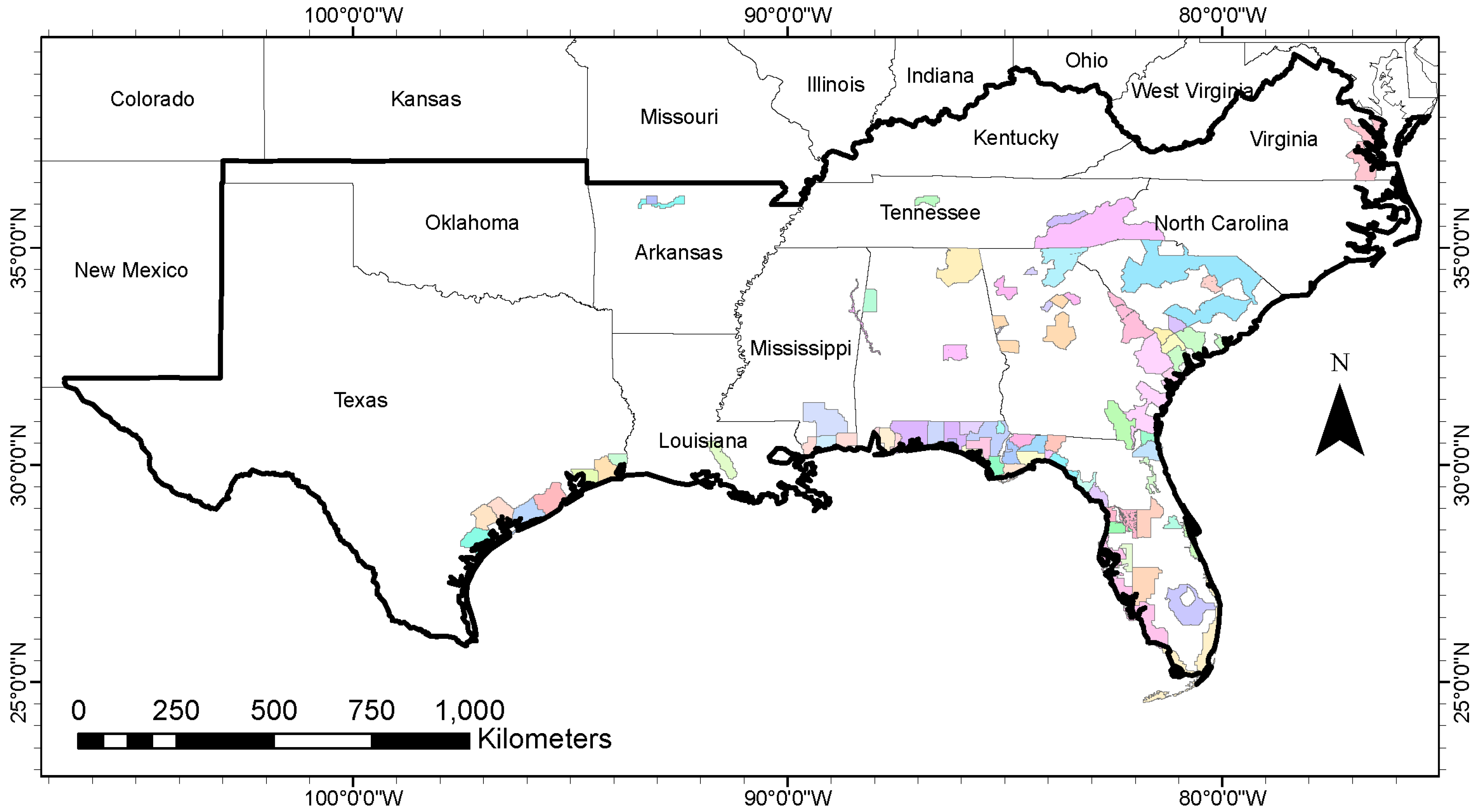
2.1. Study Area and Lidar Data Used

Our study area includes forested regions with lidar coverage for the 13 southern states of the US (Alabama, Arkansas, Florida, Georgia, Kentucky, Louisiana, Mississippi, North Carolina, Oklahoma, South Carolina, Texas, Tennessee, and Virginia). The forests in this region are quite heterogeneous, and may be broadleaf (e.g., oak-hickory and maple-beech-birch forests), or conifer forests (e.g., planted pines) or even mixed forests (e.g., oak-pine, oak-gumcypress).

We obtained regional public-domain lidar datasets archived at three agencies, as follows: (1) The U.S. Geological Survey (USGS); (2) National Oceanic and Atmospheric Administration (NOAA); and (3) Natural Resources Conservation Service (Alabama) (Figure 1). The first two agencies are the coordinating members of large data sharing partnerships, by which they store and disseminate lidar data collected by various partner agencies. For example, NOAA is the lead agency for “Digital Coast”, an initiative by which several organizations have entered into a data sharing initiative [20,21]. Many of these datasets are generated at the county-level. That is, to support engineering, hydrological and environmental studies, the public works department (or a similar department) of a given county initiates contracts with private land survey firms. These contracts are to create digital terrain models of significant parts of the county. This usually involves collecting ALS-based multiple return lidar data over the terrain. This data is then shared in the public domain, via coordinating agencies such as NOAA. Other datasets were collected by bigger agencies such as the United States Army Corps of Engineers (USACE) and the Bureau of Land Management (BLM). This heterogeneity in collection agencies is reflected in the data in terms of lidar acquisition parameters and the amount of post-acquisition quality checking done.

The lidar data were in the form of geo-referenced point clouds from 76 separate Lidar projects, with data acquisition years ranging from 2002–2012. The size of the data were around 7 terabytes (compressed). The lidar data acquired in all of these projects had multiple returns, with the maximum number of returns being four.

Figure 1. Study region—13 states of the Southeastern United States (outlined by thick black border). Lidar coverage of various projects (76 in all) is shown in different colors. The total area of lidar coverage is ~297,000 square kilometers. A total of 1755 Forest Inventory and Analysis (FIA) plots were used from this area.

Figure 1. Study region—13 states of the Southeastern United States (outlined by thick black border). Lidar coverage of various projects (76 in all) is shown in different colors. The total area of lidar coverage is ~297,000 square kilometers. A total of 1755 Forest Inventory and Analysis (FIA) plots were used from this area.

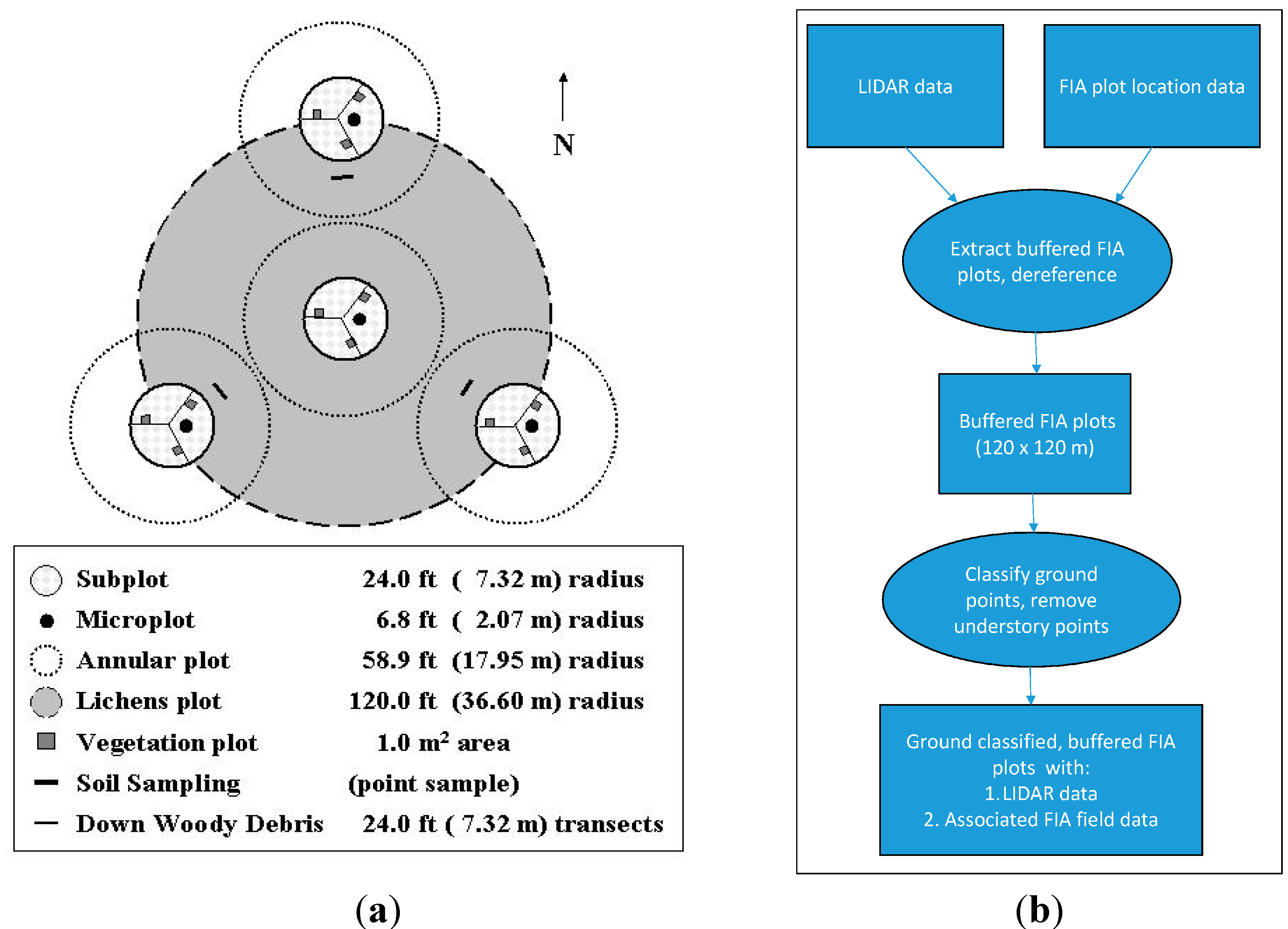
2.2. Forest Inventory Data

The Forest Inventory and Analysis (FIA) program of the United States Forest Service (USFS) is responsible for collecting nation-wide forest inventories in the US. It has been collecting field data on a nationally-standardized sampling plot since the 1990s [22]. Such plots are known as phase 2 (P2) plots, as they are used in the second phase of the three-phased inventory scheme. The quality assurance protocol used for data collection is quite robust (which will be discussed in detail later) which contributes to the usability of this dataset. The FIA P2 plot (henceforth FIA plot) layout is shown in Figure 2a. The plot location is recorded with GPS devices of variable accuracies, so co-registration with lidar data may not be always accurate. The height of all standing trees greater than or equal to 12.7 cm (5.0 inches) in diameter in the four subplots are measured; hence, plot size = ~675 m². As this plot size is relatively large and includes as much as 120–130 trees in a well-stocked area, there is a good sampling of the local canopy height by these FIA subplots. The field heights of trees were measured using clinometers. Because of practical limitations of such devices in closed canopy stands, the stated accuracy of field-based height measurements was ±10%.

Figure 2. (a) Plot layout of a standard FIA plot [23]. The height of all trees with diameter at breast height (dbh) greater or equal to 5.0 inches is measured in the four subplots shown [22]; (b) The major steps involved in the lidar data processing.

Figure 2. (a) Plot layout of a standard FIA plot [23]. The height of all trees with diameter at breast height (dbh) greater or equal to 5.0 inches is measured in the four subplots shown [22]; (b) The major steps involved in the lidar data processing.

2.3. Lidar Plot Size

For the area based approach, the sample unit is a square grid cell, and forest parameters are calculated at this resolution. It is important that the area of the ground plot and the grid cell (and hence the lidar plot) should be as similar as possible [10]. Given the spatial design of the FIA plots (see Figure 2a), it would take a square of side of at least 87.8 m to be centered on the FIA plot to cover all the four subplots. Another consideration that has to be taken into account is the error in the GPS locations of the plots, as measured by the FIA. Hence, these two criteria translate into the following:

(1)

The size of the lidar plot should be as close to that needed for the FIA plot (87.8 m).

(2)

Given the uncertainty in the spatial location of the FIA plot, the lidar plot should have a good probability of encompassing the entire FIA plot.

As for the spatial location uncertainty, an estimated probability density function of GPS errors used has been reported by scientists at the USFS FIA program [24]. This function was based upon quite extensive field trials and other considerations [25]. From this probability density function [24], we gathered that a vast majority of GPS location errors are within 15 m. Hence, we decided to use a buffer of 15 m on all sides, for meeting criteria 2 above. Hence, a good lidar plot is a square of size is 87.8 m (criteria 1) + 30 m (15 m on both sides, criteria 2) = 117.8 m. We decided to use a round number of 120.0 m, for simplicity.

2.4. Lidar Data Processing and Metrics Computed

The major steps involved in the processing of lidar data are shown in Figure 2b, and are elaborated below:

(1)

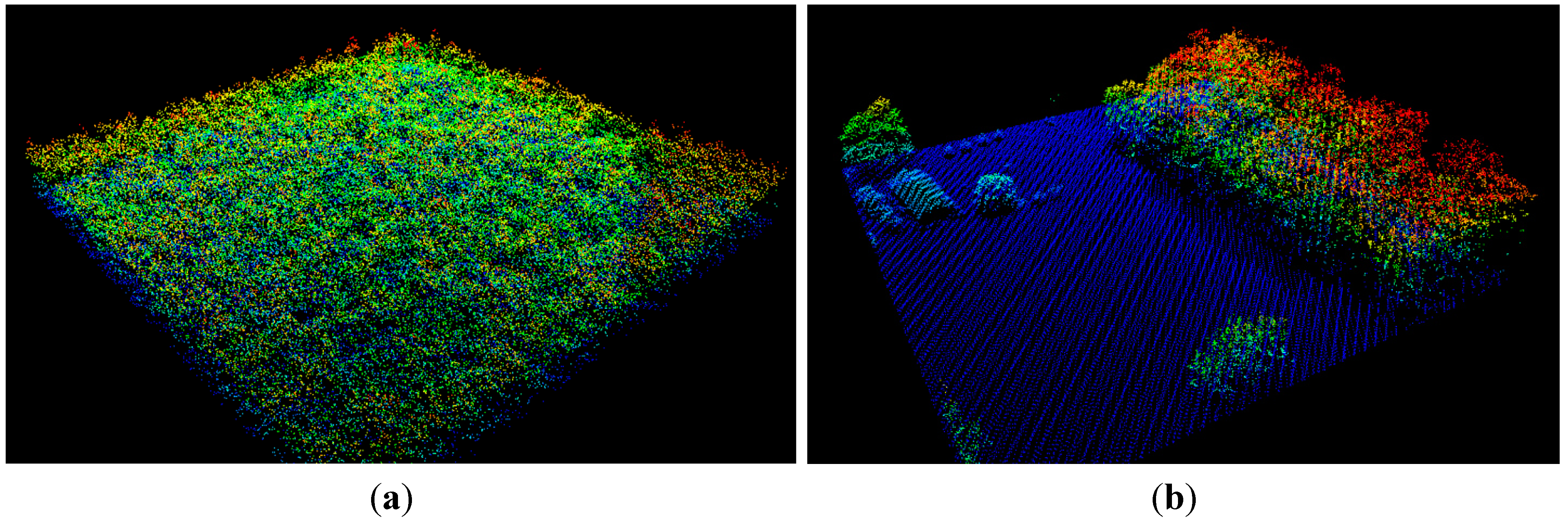
For each FIA plot location, we checked whether there was a spatially corresponding lidar acquisition within ±2 years of plot measurement. If so, lidar data corresponding to a plot encompassing the FIA plot was extracted. This was a north-south oriented square plot of length 120 m, centered at the given location of the FIA plot center. These square plots will be henceforth called the buffered FIA plots (see Figure 3). A total of 3337 such plots (corresponding to FIA plots) were cut out from the lidar point cloud data.

(2)

Ground classification on the buffered FIA plots was done using the method of progressive TIN (triangulated irregular network) densification [26], as implemented in lasground, which is part of the open-source toolset lastools (see http://lastools.org).

(3)

Understory removal: Several height thresholds have been used in the literature to remove possible ground and understory points; these range from 0.9 m [27] to 2.0 m [10,28]. We decided on the threshold of 3.0 m for the following two reasons: (a) After manual inspection of several plots for understory height, we decided that a threshold of 3.0 m was better; (b) We looked at the FIA phase 3 plots for the region, where understory heights were also measured. There, we noticed that a good proportion of shrub heights were recorded above 3 m. Hence, all points in the height bin of 0.0–3.0 m (above ground) were considered non-canopy points, and were not considered for calculation of canopy height metrics.

The resulting preprocessed data consisted of a set of plots for which we have lidar data and associated FIA individual tree heights (for the subplots). All data analysis was then performed on this set of paired elements.

Figure 3. (a) An oblique view of a buffered FIA lidar plot (120 × 120 m). The lidar point cloud is colored by elevation. Blue represents low-elevation (ground) points, while red represents higher elevations. The four circular FIA subplots of Figure 2a cover only a fraction of this area. This plot is highly homogeneous, with respect to vegetation height; (b) A highly non-homogeneous buffered FIA lidar plot, with trees clustered on the right side.

Figure 3. (a) An oblique view of a buffered FIA lidar plot (120 × 120 m). The lidar point cloud is colored by elevation. Blue represents low-elevation (ground) points, while red represents higher elevations. The four circular FIA subplots of Figure 2a cover only a fraction of this area. This plot is highly homogeneous, with respect to vegetation height; (b) A highly non-homogeneous buffered FIA lidar plot, with trees clustered on the right side.

Several metrics (descriptive lidar metrics and otherwise) were computed over the buffered FIA plots, and for the FIA data:

(1)

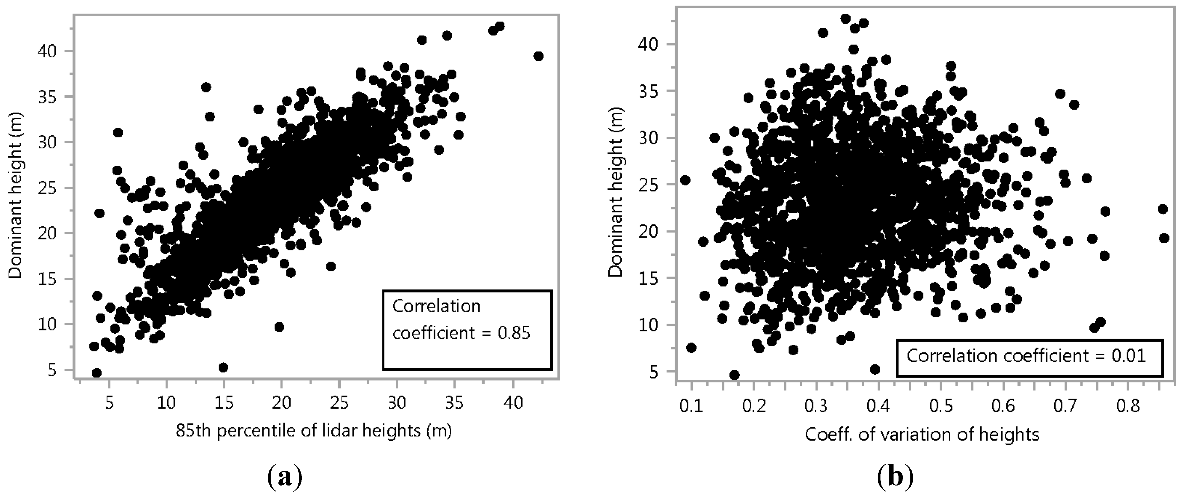
Lidar distributional metrics for canopy height: Height percentiles have been shown to be significant canopy height predictors in previous related efforts [10,27]. Hence, the major percentiles (5th, 10th, 15th, 20th …) of the heights (above ground) of canopy first returns (i.e., greater than 3.0 m from the ground) over the buffered FIA plots were calculated. These are denoted as h₅, h₁₀, h₁₅, etc. We also calculated the coefficient of variation of the heights of canopy first return points, as it has shown to be significant in such models [27]. This metric is denoted as cv_canPts.

(2)

Plot homogeneity: This quantifies the homogeneity of distribution of vegetation height in the area around the FIA plots. The importance of this metric will be explained in the next section. For computing it, we divide the buffered FIA plot into 144 square units, each of area 100 m². This was done by using a regular grid pattern. Then, we calculate the 85th percentile of heights of all returns (including understory) for each of those 144 square units. Finally, we calculate the coefficient of variation of these 144 values (henceforth CV), which is a normalized quantification of the amount of dispersion of vegetation heights over the plot. Hence, given that (h₈₅)_i is the 85th percentile height of all lidar returns for the ith square unit, the CV at the plot level is calculated as:

$$CV=\frac{{\left(\frac{1}{143}{\displaystyle \sum _{i=1}^n{\left({\left(h_{85}\right)}_i-\overline{h_{85}}\right)}^2}\right)}^{1/2}}{\overline{h_{85}}}$$

(1)

$$\text{where} \overline{h_{85}}=\frac{{\displaystyle \sum _{i=1}^{144}{\left(h_{85}\right)}_i}}{144}$$

(2)

We include the understory points in this calculation because we hypothesize that the amount of homogeneity of the entire vegetation structure (including the understory) on the 120 m square plot is instrumental to good correlations between lidar and field measured metrics. This is because the presence of understory vegetation plays a role in determining how well ground detection algorithms work.

(1)

Scan angle: The average scan angle, in degrees, as recorded in the lidar metadata. Additionally, we flagged plots that had lidar data with either no scan angle recorded or had scan angles improperly recorded. Also, we flagged plots where the lidar data were from multiple flight lines (hence, averaged scan angles are not representative). These were marked with a “no good scan angle information” flag.

(2)

Slope of the buffered FIA lidar plot: This is the average slope, expressed in degrees, measured in the field by the FIA crew.

(3)

The dominant tree height of all the trees measured by FIA on the subplots. The dominant tree height (henceforth “dominant height”) is the average height of the five tallest trees in the four FIA subplots. Note that this definition differs from the more common definition used in forestry. We used this definition to maintain consistency across all plots.

(4)

We also estimated the effect of broad species grouping (softwood vs. hardwood) on the models. Softwood trees include evergreen conifers such as pines, spruces and cedars, while hardwoods include deciduous trees such as oaks, maples and birch. The FIA field crew also records species data for all trees measured. We used that information to estimate the percentage (by basal area) of softwoods in the four FIA subplots. That is, we defined and calculated percent_softwood using the following formula:

$$\mathit{\text{percent\_softwood}}=\frac{\left({\displaystyle \sum _{i=1}^m{\left(BA\right)}_i}\right)\times 100.0}{\left({\displaystyle \sum _{i=1}^n{\left(BA\right)}_i}\right)}$$

(3)

where (BA)_i = the basal area of the ith tree; m = number of softwood trees on the plots; (summation over all softwood trees); n = total number of trees on the plot; (summation over all trees)

2.5. Accounting for Plots with Multiple Land Use Conditions

For a land use parcel to be classified as forest by the FIA, it must be at least 10 percent stocked with tree species, at least 1 acre in size, and at least 120 feet wide [22]. An important aspect of the FIA plot design (fully randomized plot locations) is that plots can potentially straddle multiple land use types (called “conditions” in the FIA literature). For example, one could have a plot where 40% (by area) is forested, 40% is nonforested (agricultural land) and 20% is water (rivers, lakes, etc.). Such randomized locations are needed for truly unbiased estimates with no domain misclassifications [22]. Forest land also includes transition zones, such as areas between forest and nonforest lands that meet the minimal tree stocking requirement. Unimproved roads and trails, streams, and clearings in forest areas are also classified as forest if they are less than 36.6 m (120 feet) wide or less than 0.4 hectares (an acre) in size. But as our modeling effort was focused on forested regions, we selected a subset of FIA plots with predominant forested land use at the time of measurement, defined as follows: (a) Over 90% of the land use was classified as “forested”; (b) There were at least three trees on each of the four FIA subplots. These two conditions resulted in the selection of 1755 FIA plots (from the 3337 plots discussed in Section 2.4.), and all subsequent analysis and modeling were restricted to data from these plots.

2.6. Main Model Specification

We developed an OLS (ordinary least squares) based bivariate linear regression model based on data from the 1755 plots mentioned above. All variables were estimated at the buffered FIA plot level. We considered the dominant tree height of all the trees measured by FIA on the subplots as the response variable. The following predictor variables were considered:

(1)

A height percentile from lidar canopy first returns (from the set of h₅, h₁₀, h₁₅, h₂₀, etc). The percentile chosen was the one most correlated to the dominant height.

(2)

cv_canPts, the coefficient of variation of the heights of canopy first returns.

We chose a simple model with no data transformations as our primary interest was in the regression residual analysis for factor importance. Also, a simple model is less prone to overfitting [29], which is essential when one plans to extend the model over a large area. Before constructing the model, we assessed the assumptions of linear regression (near-linear trend, normality of distribution of variables, homogeneity of variances) with both the explanatory and response variables to ensure that the model choice was appropriate. Then, the model was developed and standard goodness-of-fit metrics like the coefficient of determination (R²) and root mean square error (RMSE) were calculated.

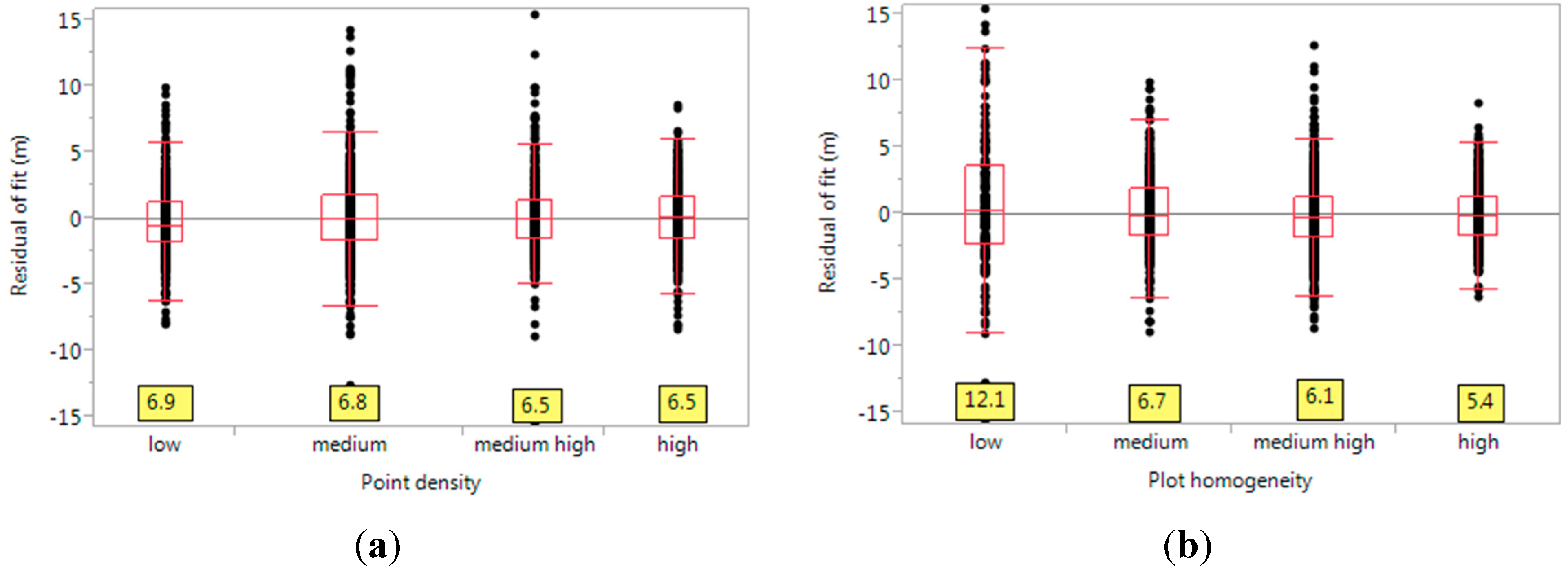
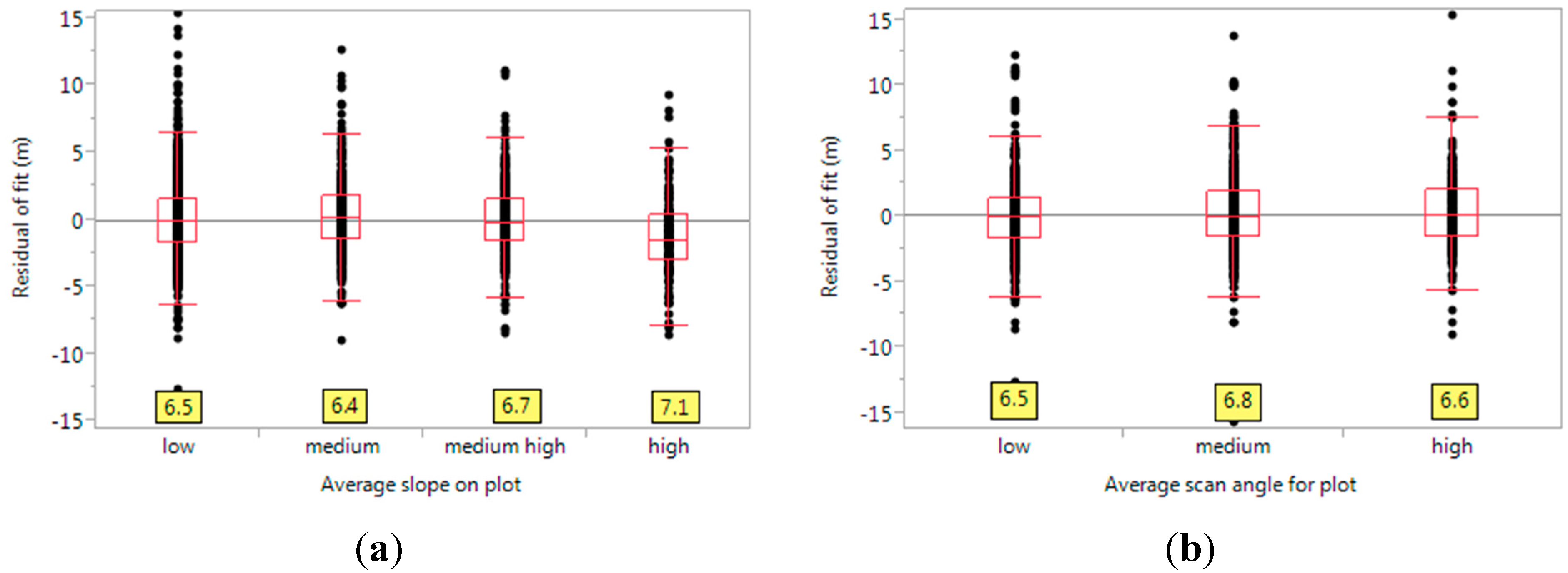
2.7. Factors Affecting Efficacy of Prediction

The objective of this stage of analysis was to understand the relative importance of several factors in affecting the efficacy of the main model. We considered the following factors:

(a)

Point density of lidar returns (all returns), over the buffered FIA plot. This is expressed as (number of returns)/m².

(b)

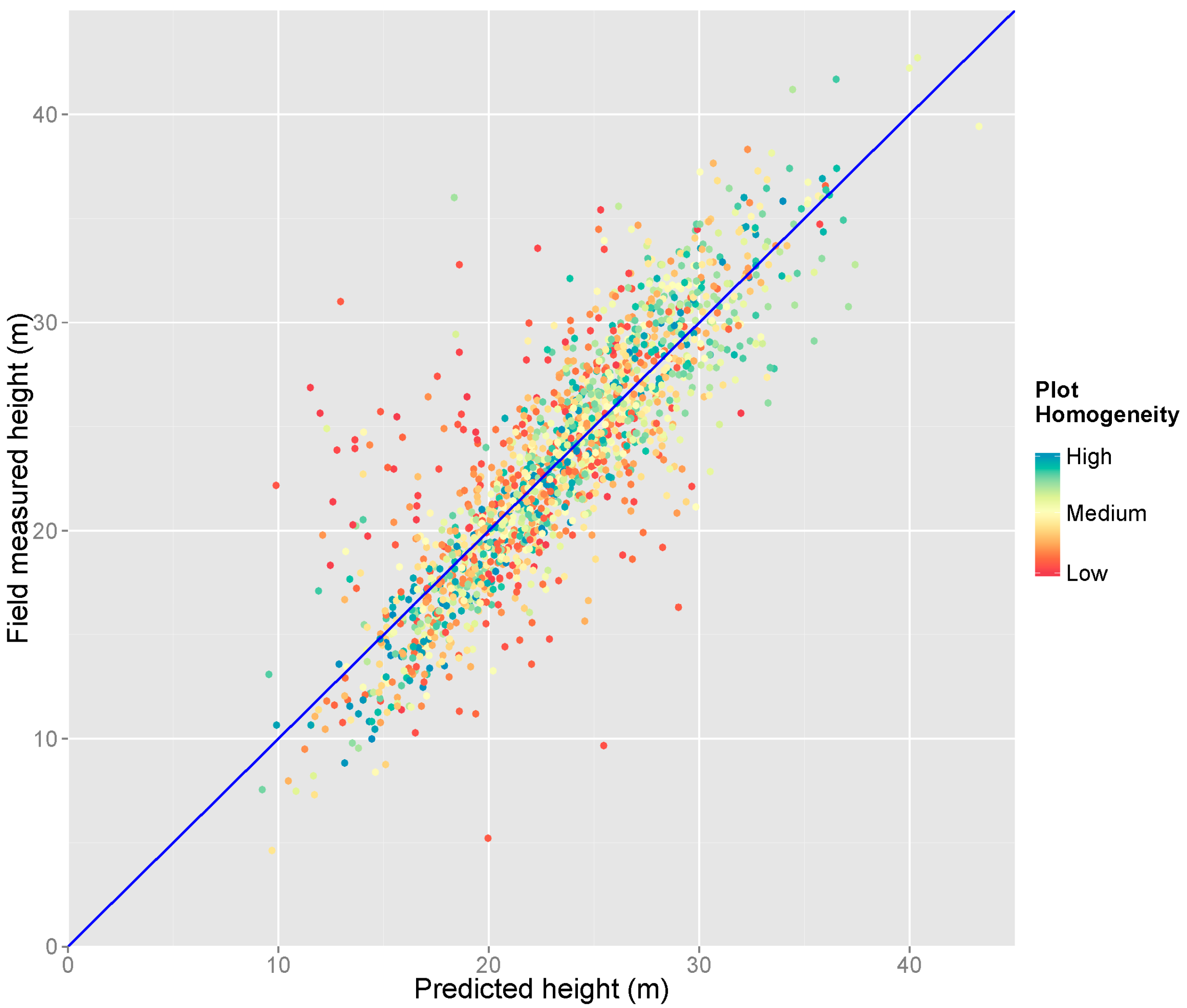
Plot homogeneity, estimated from lidar returns (quantified by CV).

(c)

Percent softwood (estimated from FIA field data).

(d)

Average height of trees (estimated from FIA field data).

(e)

Slope of the plot terrain (estimated from FIA field data).

(f)

Average lidar pulse scan angle (estimated from lidar metadata).

Such an analysis can have three potential uses: (1) Understand the importance of lidar acquisition parameters (like point density) on the robustness of the models involved; (2) Understand how the study area characteristics affect model performance; (3) Help in the stratification of the study area, for better confidence intervals of parameter estimates. It is important to recognize that the above list is not exhaustive with respect to factors that could possibly affect model performance. Nevertheless, we were constrained by factors that were consistently available across all 76 projects involved. We used regression residual analysis to analyze the relative importance of the above factors in effecting deviations from a linear fit. Such analysis is useful in understanding the factors that affect the main model [30,31]. We made standard boxplots of the residuals for various ranges of the factors involved. If the spread (variance) of the residuals were affected by the level of the factor at hand, it indicates that the factor is important to model canopy heights. That is, (for example) if plots with low point density had a bigger spread of residuals than plots with higher point density, it indicates the importance of point density in effecting lower residuals. We used the Brown-Forsythe test, a formal nonparametric test for homogeneity of variances to test the significance of our measured difference in variance, or spread [32].

For another independent assessment of the relative importance of factors above, we also used the Random Forest (RF) algorithm, a novel and powerful extension of classification tree techniques. Variable importance is determined in this technique by changing the data for a given variable and noting the increase in prediction error. The random forest algorithm has been shown to produce excellent results in classifications of remotely sensed and ecological data [33]. We used the RF package (version 4.6–10) [34] in R (www.r-project.org). The predictor variables were those used in the main model plus five of the six factors listed above (the average height of trees was excluded, explained below). The response variable was dominant height, same as that used in the main model. The average height of trees was excluded, as it is highly correlated with the response variable. A subset consisting of a random selection of 70% of the plots was used for training, and the rest (30%) of the plots used for testing. This process was repeated 10 times and the results were averaged. First, the robustness of the model was verified by comparing the RMSE (generated using the testing subset) with the RMSE of the main model. Then, the relative importance of each of the six factors above were recorded. For this exercise, we had to exclude plots that had the “no good scan angle information” flag set. Hence, we could use only the 1153 plots where all required independent variables were available.

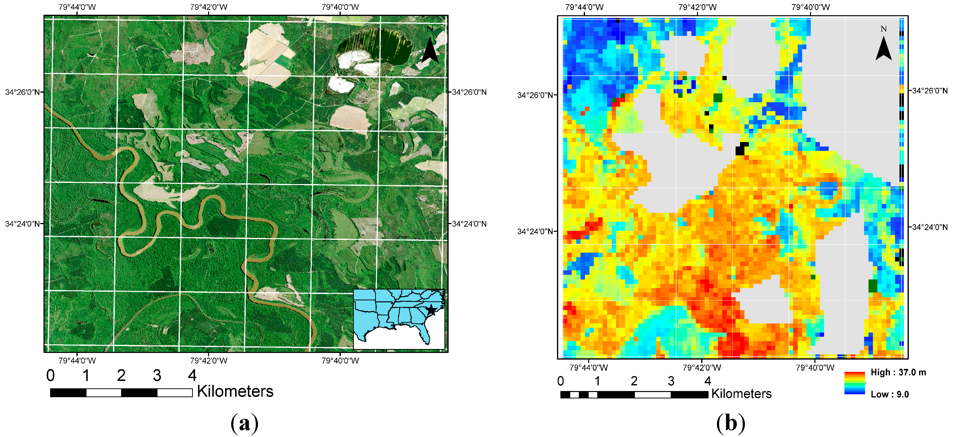
2.8. Generation of Sample Canopy Height Map

Recent papers have detailed the area-based approach, a methodology to derive wall-to-wall maps of forest parameter estimates from Lidar data [9]. There have been several efforts that have successfully generated such maps [35]. There are two essential stages involved in this approach. During the first stage, ALS data is acquired over the region of interest, along with vegetation measurement data from sample ground plots. Then, predictive models are developed between the ALS data and ground measurements. In the second stage, the ALS metrics used for model construction are calculated over the entire wall-to-wall area. Here, the sample unit would be a grid cell, roughly corresponding to the size of plots used for the models. Then, the predictive model is applied at each sample unit to get the map of forest parameter estimates. A wall-to-wall forest canopy height map of a large portion of the southeastern US generated at the end of this stage would be very useful to forest scientists and the forest management community. However, we realized that implementing the second stage described above was non-trivial for us. That is, designing, implementing, and testing the software system to process seven terabytes of lidar data, then validating the end products, was beyond the scope of this study. Also, there would be significant computation time involved. Hence, this paper concentrates on the first stage (developing predictive models). We also decided to generate a canopy height map for a relatively small area (9.2 × 9.2 square kilometers), to test out the predictive model developed. Specifically, an area straddling Darlington and Marlboro counties in the state of South Carolina was chosen. This area had the following advantages: (1) The lidar coverage over that area was from a project that was quite representative of our lidar dataset; the acquisition was done in 2008, with a point density of 2–3 points/m²; (2) We had access to high-quality aerial orthophotography for that area from the summer of 2009; (3) Due to the presence of various land-cover features such agriculture, managed tree plantations, natural forests, a river and some lakes, one could expect a good range of forest stand heights; (4) At such small scales, landscape level patterns are quite discernible. Hence, we could compare broad features of our map to high-resolution aerial orthographic photos.

The map was made with the following steps:

Step 1: Divide the area into grid-cells of size 120 × 120 m.

Step 2: Identify non-forest grid cells (urban, agriculture, water) and flag them as “non-forested”, with all other grid cells labelled “forested”. This was done by visual inspection of the associated high-resolution image. But, on a larger scale, this can be done by using existing land-classification products such as the National Land Cover Dataset (NLCD) of the United States [36].

Step 3: Calculate descriptive lidar metrics for all the forested grids, as described in Section 2.4 above. Then, compute the grid-level predicted dominant height by using the main model. Note that we use only lidar first-returns above a threshold of 3.0 m for computation of lidar metrics (to remove understory points). There might be some grid-cells in our region that have no points above this threshold. We do not use the predictive model for such points, and denote their canopy height as zero. In other words, these are marked as “pure understory” grid cells.

3. Results

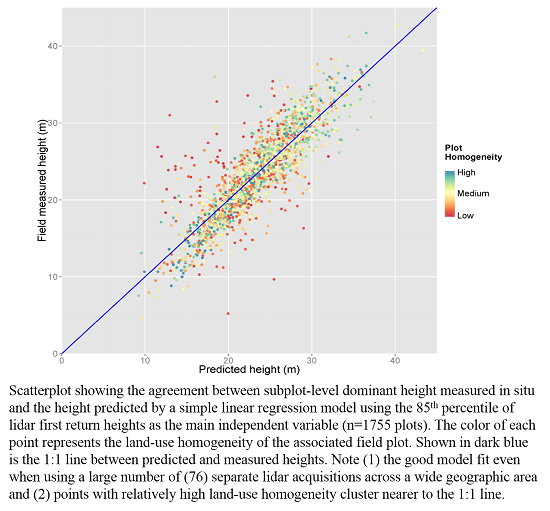
3.1. Main Model

After examining the correlations between plot-level lidar distributional metrics and dominant tree heights, the 85th percentile (h₈₅) of lidar heights were selected. Hence, dominant tree height was used as the dependent variable (dom_tree_ht below), while h₈₅ and cv_canPts were tried out as candidates independent ones. The final OLS based linear regression model has the form:

dom_tree_ht = 5.658 + 0.859 × h₈₅ + 3.776 × cv_canPts

(4)

The R² of the fit was 0.74 and the RMSE (root mean square error) was 3.0 m. Both independent variables were highly significant (p < 0.0001). Their individual correlation with dominant height can be seen in Figure 4. As the independent variables had the ranges of 3.0 < h₈₅ < 42.0 and 0.09 < cv_canPts < 0.85 for model calibration, the model is only valid for these variable ranges.

Figure 4. (a) Correlation between the 85th percentile of lidar first return heights and the FIA-measured average dominant tree height (n = 1755 plots) (b) Correlation between the coefficient of variation of the heights of canopy first returns (cv_canPts) and the FIA-measured average dominant tree height (n = 1755 plots).

Figure 4. (a) Correlation between the 85th percentile of lidar first return heights and the FIA-measured average dominant tree height (n = 1755 plots) (b) Correlation between the coefficient of variation of the heights of canopy first returns (cv_canPts) and the FIA-measured average dominant tree height (n = 1755 plots).

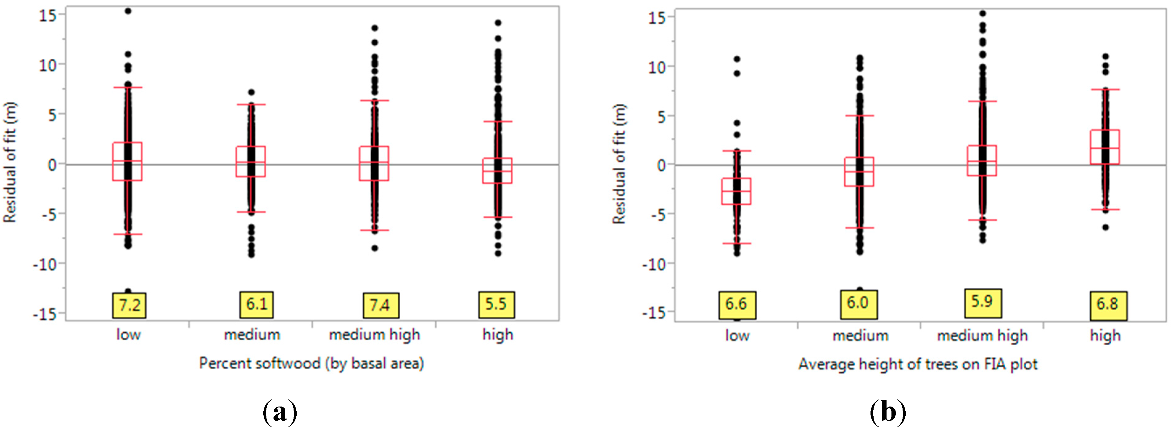
3.2. Variable Importance for Goodness of Fit

As mentioned in Section 2.8, we analyzed the residuals of the linear fit above with respect to various factors. To study the effect of point density on the residuals, we made a standard boxplot of the residuals for various ranges of point density values (Figure 5a). The slight effect of better point density to affect better fits can be seen here, albeit quite muted. That is, the spread of residuals (measured by the difference in quantiles) changes slightly from 6.9 to 6.5 m, when one moves from low to high point density. Also, we do not detect significant differences in the variance of the residuals at various levels used, using the Brown–Forsythe test (test statistic = 2.174, p-value = 0.089). Nevertheless, the importance of point density has been noted in various previous papers: The authors in [17] report that point density had even greater influence than footprint size on canopy height estimates. The relative unimportance of this variable for us may be due to our large plot size, which guarantees a sufficiently large number of returns even with low point density. The effect of plot homogeneity can be seen in Figure 5b. Plots with low homogeneity (such as the one in Figure 3b) have higher spread of residuals, whereas more homogeneous plots (Figure 3a) are well-modelled by the linear fit. The quartile range decreases by as much as 6.7 m (from 12.1 to 5.4) between the two extremes, in this case. This highlights the considerable importance of plot homogeneity in explaining the lack-of-fit of several plots. Also, the Brown-Forsythe test points to significantly high differences in the variances (test statistic = 55.05, p-value < 0.001). Hence, we note that the effect of plot-level vegetation heterogeneity is pronounced in this set of plots.

Figure 5. (a) The effect of point density on the residuals of the linear fit. Here, “low” denotes point densities of 0.25–0.5 points/m², “medium” is 0.5–2.0, “medium high” is 2.0–4.0, and “high” is above 4.0_. The values at the bottom (yellow boxes) are the quantile ranges, between the 10th and the 90th quantiles (this is same for other figures). They represent the spread of the residuals, for various ranges of point density. Higher point density has the effect of reducing the range of residuals, giving a better fit; (b) Effect of plot homogeneity on the residuals. We use coefficient of variation (CV) to quantify plot homogeneity, where higher CV values denote lower plot homogeneity. Here, the label of “low” homogeneity denotes CV values above 0.5, “medium” is 0.3–0.5, medium high is 0.15–0.3, and high is CV below 0.15_. The significant shrinking of the quantile range (from 12.1 to 5.4 m) for increasing plot homogeneity is notable.

Figure 5. (a) The effect of point density on the residuals of the linear fit. Here, “low” denotes point densities of 0.25–0.5 points/m², “medium” is 0.5–2.0, “medium high” is 2.0–4.0, and “high” is above 4.0_. The values at the bottom (yellow boxes) are the quantile ranges, between the 10th and the 90th quantiles (this is same for other figures). They represent the spread of the residuals, for various ranges of point density. Higher point density has the effect of reducing the range of residuals, giving a better fit; (b) Effect of plot homogeneity on the residuals. We use coefficient of variation (CV) to quantify plot homogeneity, where higher CV values denote lower plot homogeneity. Here, the label of “low” homogeneity denotes CV values above 0.5, “medium” is 0.3–0.5, medium high is 0.15–0.3, and high is CV below 0.15_. The significant shrinking of the quantile range (from 12.1 to 5.4 m) for increasing plot homogeneity is notable.

We also calculated the effect of species grouping (softwood vs. hardwood) by estimating percent_softwood, the percentage (by basal area) of softwoods in the stand. These values were then binned and corresponding boxplots were generated (see Figure 6a). For example, the bin of low denotes that the softwood basal area is less than 25% of the total basal area, or that the stand is dominated by hardwoods. Likewise, medium is for basal area of 25%–50%, medium high is for 50%–75% and high is for 75%–100% (mostly softwoods). Here, it can be seen that hardwood stands are associated with higher quantile range than softwoods. This is because all our lidar acquisitions were done in a leaf-off vegetation state. On the other hand, when the stands were dominated by softwoods, the quantile range decreased by 1.7 m (from 7.2 to 5.5). These results are similar to those of [37], where it was reported that percentile methods have problems in estimating height in deciduous compound canopies during leaf-off conditions. Again, it was reported that model predictions improve when the study area is stratified into softwoods and hardwoods, with softwoods generating better R² values [14]. Also, the Brown-Forsythe test shows significant differences in variances (test statistic = 7.281, p-value < 0.001).

Another factor of importance is the average height of the trees in these stands (which is an indicator of the age class of the trees). This is explored in Figure 6b. For a stand with short trees, we over-predict height whereas we under-predict for tall trees. We attribute this to two reasons: (1) Tall trees indicate mature stands with more shrubs and understory, increasing the chance of errors in ground classification; (2) When the trees measured on the subplots are tall, they have higher probability to be the dominant trees in the buffered FIA plot (and to be associated with the 85th percentile of lidar returns). This also suggests that a better model may be a piecewise linear one, with a segment for the low tree height, another for the medium and medium high tree heights and one for the high tree heights. In general, we can see that there is very less difference between the variances for various levels of the factor. This is confirmed by the Brown-Forsythe (test statistic = 0.461, p-value = 0.709), indicating that average height of trees is not a significant factor regarding our model’s inaccuracy.

Figure 6. (a) The effect of species groups (softwood vs. hardwoods) on the residuals. The values at the bottom (yellow boxes) are the quantile ranges, between the 10th and the 90th quantiles. Here, softwood basal area is used for the categories. That is, “low” indicates a softwood basal area of 0%–25%, medium is 25%–50%, medium high is 50%–75% and high is more than 75%. The quantile range is much greater in the hardwoods case; (b) Effect of height of the stand on the residuals. The x-axis represents the average height of all trees measured by the FIA (in the four subplots). Here, “low” denotes stand height of 0–10 m, “medium” is 10–15 m, “medium high” is 15–20 m and “high” is more than 20 m.

Figure 6. (a) The effect of species groups (softwood vs. hardwoods) on the residuals. The values at the bottom (yellow boxes) are the quantile ranges, between the 10th and the 90th quantiles. Here, softwood basal area is used for the categories. That is, “low” indicates a softwood basal area of 0%–25%, medium is 25%–50%, medium high is 50%–75% and high is more than 75%. The quantile range is much greater in the hardwoods case; (b) Effect of height of the stand on the residuals. The x-axis represents the average height of all trees measured by the FIA (in the four subplots). Here, “low” denotes stand height of 0–10 m, “medium” is 10–15 m, “medium high” is 15–20 m and “high” is more than 20 m.

We also calculated the effect of slope of the FIA plot (see Figure 7a). In this case, the Brown-Forsythe test only shows slight differences in variances (test statistic = 0.668, p-value < 0.572). Our model over-predicts heights on steep slopes. This may be due to the fact that these plots correspond to mountainous terrain, where there is usually more softwoods, for which our model over-predicts (see Figure 6a). Another reason may be the relative lack of understory on these drier sites. The effect of scan angle on the residuals is seen in Figure 7b. The relative lack of effect of both these factors on the spread is mostly due to the large plot size used. This guarantees that the distributions are fairly stable over such changes.

Figure 7. (a) The effect of average slope of the FIA plot the residuals. The values at the bottom (yellow boxes) are the quantile ranges, between the 10th and the 90th quantiles. Here, “low” indicates a slope of 0 or 1 degrees, medium is a slope of 1–10 degrees, medium high is 10–25 degrees and high is more than 25. The quantile ranges are similar, but higher for steeper plots; (b) Effect of lidar scan angle on the residuals. The x-axis represents the average scan angle, as recorded in the lidar metadata. Here, “low” denotes scan angles from 0 to 5 degrees, medium from 5 to 12 degrees, and high above 12 degrees.

Figure 7. (a) The effect of average slope of the FIA plot the residuals. The values at the bottom (yellow boxes) are the quantile ranges, between the 10th and the 90th quantiles. Here, “low” indicates a slope of 0 or 1 degrees, medium is a slope of 1–10 degrees, medium high is 10–25 degrees and high is more than 25. The quantile ranges are similar, but higher for steeper plots; (b) Effect of lidar scan angle on the residuals. The x-axis represents the average scan angle, as recorded in the lidar metadata. Here, “low” denotes scan angles from 0 to 5 degrees, medium from 5 to 12 degrees, and high above 12 degrees.

3.3. Variable Importance from the Random Forest Model

We generated a random forest model using 1153 plots (see Section 2.7.). The model was quite robust, yielding an RMSE of 2.87 m with independent test data. The variable importance values are given in Table 1. One can note that the relative variable importance values differs from those from the main model. This is mostly because of the additional variables available to the random forest model. For example, it used the “percent softwood” variable and that variable was able to explain some of the variance in CV (for example, mixed stands of evergreen and deciduous trees can be expected to have higher CV). But the relative trends are the same. That is, plot homogeneity (as quantified by CV) and percent softwood are important variables for modeling stand heights, followed by slope. Scan angle and point density are not important at this plot size. The relative importance of these factors is useful to keep in mind when one tries to improve the precision of height estimates by stratification techniques. Plot slope, in general, has been found to be important previously too: For individual tree heights, it has been reported that underestimates of tree height were larger on lower elevations (−0.85 m) than on higher elevations (0.17 m) [38]. The importance of slope for the accuracy of Lidar-derived tree detection has also been studied [39]. It was reported that the accuracy of tree detection is 74% for steep slopes but is 86% for gentle slopes.

As plot homogeneity was established in the above analysis as an important variable, we examined its efficacy in explaining residuals of our main model in Figure 8. It can be seen that points with relatively high land-use homogeneity cluster nearer to the 1:1 line, and are hence better modeled. Again, most of the points far from the 1:1 line (i.e., not well modeled by us) have low plot homogeneity.

Table 1. The variable importance values of the random forest model generated. The importance of a variable is estimated by seeing how much the prediction error increases when that variable is permuted, keeping all else unchanged [34]. The variables at the top of the table are more important. The Brown–Forsythe test statistic (which quantifies the spread of residuals of our main model) is also given for reference. NA: Not Applicable.

Variable	Increase in Error (%)	Brown-Forsythe Test Statistic
h85	113.2	NA
Percent softwood	22.3	7.28
CV (measure of plot homogeneity)	15.0	55.05
cv_canPts	14.3	NA
Slope	9.0	0.67
Point density (PD)	4.2	2.17
Scan angle	3.3	0.41

Table 1. The variable importance values of the random forest model generated. The importance of a variable is estimated by seeing how much the prediction error increases when that variable is permuted, keeping all else unchanged [34]. The variables at the top of the table are more important. The Brown–Forsythe test statistic (which quantifies the spread of residuals of our main model) is also given for reference. NA: Not Applicable.

Variable	Increase in Error (%)	Brown-Forsythe Test Statistic
h85	113.2	NA
Percent softwood	22.3	7.28
CV (measure of plot homogeneity)	15.0	55.05
cv_canPts	14.3	NA
Slope	9.0	0.67
Point density (PD)	4.2	2.17
Scan angle	3.3	0.41

Figure 8. Scatterplot showing the agreement between subplot-level dominant height and the height predicted by our main model (n = 1755 plots). The color of each point indicates the land-use homogeneity of the field plot associated with it (measured by CV). The dark blue line is the 1:1 line between predicted and measured heights.

Figure 8. Scatterplot showing the agreement between subplot-level dominant height and the height predicted by our main model (n = 1755 plots). The color of each point indicates the land-use homogeneity of the field plot associated with it (measured by CV). The dark blue line is the 1:1 line between predicted and measured heights.

3.4. Sample Canopy Height Map

A sample canopy height map was generated over a 9.2 × 9.2 square kilometers area, as described in Section 2.8. (Figure 9). The range of dominant canopy heights that we generate (37 m) is reasonable for the area at hand: Loblolly pine is known to grow to a height of ~40 m in that region. Also, the spatial variation in canopy height seems to follow expected patterns on the landscape. The heterogeneity in vegetation heights along the river is picked up by the CV (dark green) pixels, as expected. These results indicate that a wall-to-wall canopy height model with bounded uncertainty can be generated from our lidar dataset.

Figure 9. (a) A high-resolution aerial photo of the area used for verification of the model. The image is from the National Agriculture Imagery Program (NAIP) of the United States Department of Agriculture, acquired during the summer of 2009. The inset shows the location of the area in southeast United States. The coordinates of the center of the area are 34.410016N, 79.690276W (latitude, longitude; using WGS 84 datum). The white lines demarcate lidar data “tiles”, each of ~1.8 km wide; (b) Canopy height map for the area generated using our main model. The height is denoted in m, and the faint white lines correspond to the lidar data tiles, same as shown in Figure 9a. The grey area is non-forested land, the black pixels are “pure understory”, and the dark green pixels are where lidar metrics are otherwise beyond the range of our model (hence, the model is not applicable).

Figure 9. (a) A high-resolution aerial photo of the area used for verification of the model. The image is from the National Agriculture Imagery Program (NAIP) of the United States Department of Agriculture, acquired during the summer of 2009. The inset shows the location of the area in southeast United States. The coordinates of the center of the area are 34.410016N, 79.690276W (latitude, longitude; using WGS 84 datum). The white lines demarcate lidar data “tiles”, each of ~1.8 km wide; (b) Canopy height map for the area generated using our main model. The height is denoted in m, and the faint white lines correspond to the lidar data tiles, same as shown in Figure 9a. The grey area is non-forested land, the black pixels are “pure understory”, and the dark green pixels are where lidar metrics are otherwise beyond the range of our model (hence, the model is not applicable).

4. Discussion

4.1. The Influence of Co-Registration Issues

Good geographical co-registration of lidar and field plot data is essential for accurate prediction of forest stand biophysical properties from a lidar point cloud [40,41]. The location of FIA field plots are determined by GPS instruments whose positional accuracies are determined by a host of factors such as equipment, user, satellite, atmospheric and environmental [42]. Moreover, GPS signals are easily blocked or scattered by forest canopies (which often leads to multipathing) and hence it is problematic to get horizontal accuracies of less than 5 m on plot locations [43,44]. Hence, the error in our model is due to two reasons: (1) The inability of lidar to fully characterize the canopy profile. This may be due to factors such as incorrect estimation of the ground, undersampling of tall trees, lidar returns disproportionately reflected from the lower branches, and sensor errors; (2) The mismatch between the FIA and the lidar plots. The shape and size of the FIA and the lidar plots are different. The lidar plot needed to be designed this way to make sure that it had a good probability of containing the FIA plot. A consequence of this is that these plots could be covering very different patches of forests. For example, the FIA subplots may be over a patch of very tall pine trees, while there may be mostly very short beech trees over the lidar plots.

For understanding the effect of co-registration errors (and augmented plot size required), consider any of the 1755 lidar plots used for our main models. The total error of our estimate of canopy height for that plot has the following three components:

E_total = E_model + E_{non-representative-subplots} + E_{FIA-measurements}

where:

• E_total is the total error, which is the difference between the actual dominant height of the forest patches on that lidar plot, and that predicted by our models.
• E_model is the error in modelling the dominant height of the trees on the FIA subplots from the lidar data, on the lidar plot. This is captured by the RMSEs of our models, and may be due to several factors, as discussed in Section 2.7.
• E_{non-representative-subplots} is the error caused by the fact that the dominant height of the trees on the FIA subplots (that we model) is not the same as the dominant height of the trees over the entire lidar plot. The difference can sometimes be large, may be due to the fact that the FIA subplots may be sampling a patch of forest with very different characteristics (see above) or that most of the area of the subplots could be outside the lidar plot (due to very high co-registration errors). But in general, this error term is expected to be lesser in areas where vegetation is more homogeneous. There have been recent reports that LiDAR metrics are less sensitive to co-registration errors in dense, spatially homogeneous stands than sparse, heterogeneous stands [40]. However, further work is needed to quantify this term.
• E_{FIA-measurements} is the error in the FIA measurement, recording and processing of tree heights. We assume this to be relatively so small as to be negligible.

Given the adequate sampling of the area of interest by the large number of plots, it can be expected that the error for any grid cell of generated maps (such as those in Figure 9a) would be the same as E_total above. Also, in the absence of significant co-registration issues, the lidar point cloud over just the FIA subplots could have been extracted (instead of extracting a bigger buffered plot). In this case, the term E_{non-representative-subplots} would be zero.

In a recent paper, it has been pointed out that in spite of the increasing acceptance of airborne lidar in forest research and operational forest management, there have been only a few published studies examining the impact of co-registration error on the prediction accuracy of regression estimators [40]. In that study, the authors examined various factors (mainly plot size and co-registration errors) contributing to the successful development of spatially extendable regression models. They used a large dataset (n = 179) of computer-generated coniferous forest canopies to conclude that regression models using larger plots (area of plot = 707 m²) were substantially more robust to the ill-effects of co-registration errors. Goodness-of-fit values like R² and RMSE (of the biomass, in this case) were shown to be less affected when the plot size was increased. For example, when the plot size was increased from 314–1964 m², the RMSE of forest biomass prediction expressed as a proportion of average biomass went down from 47% to 34%. In this context, FIA’s relatively large plot size works to our advantage. There have also been recent attempts to correct FIA plot locations using high-density lidar data (which is assumed to have minimal registration errors) [45]. This is done by identifying and matching individual tree crowns between the two datasets. But such efforts are not scalable, as the spatial extent of high-density lidar data (in which distinct individual trees can be identified) remains small.

4.2. Lidar-Based Grid Cell Homogeneity

A significant finding of this work was the efficacy of a lidar-based homogeneity metric in explaining the errors of our model. The CV metric was found to be important both in the main model and in the random forest model. To further study this, we considered two subsets of plots, which are more homogeneous: (a) CV < 0.5; (b) CV < 0.2. We developed OLS based linear regression models for these plots with dom_tree_ht as the dependent variable and h₈₅, cv_canPts as the independent ones. The results of this exercise are summarized in Table 2. Hence, if one considers only areas of higher homogeneity (such as CV < 0.2), the RMSEs involved can be much lower, such as 2.44 m. These RMSEs only represent the E_model term (see Section 4.1., above). But it can be reasonably expected that the E_{non-representative-subplots} term is also lower in homogeneous forest areas. If one assumes that E_{non-representative-subplots} term is nearly zero when CV < 0.2, the E_total of the model is close to 2.44 m. This is comparable to recent estimates for much smaller areas: Erdody and Moskal reported an RMSE of 1.9 m for tree heights using lidar (n = 57) [27]. Also, the percent of original number of plots in the new subset gives an indication of the percent of the grid cells for which this new “homogeneous” model can be used.

Table 2. Goodness of fit statistics of models based on sets of more homogeneous plots.

CV Threshold	Number of Plots	% of Original Num. Plots	R2	RMSE (m)
CV < 0.5	1573	89.6	0.81	2.60
CV < 0.2	729	41.5	0.84	2.44

Table 2. Goodness of fit statistics of models based on sets of more homogeneous plots.

CV Threshold	Number of Plots	% of Original Num. Plots	R2	RMSE (m)
CV < 0.5	1573	89.6	0.81	2.60
CV < 0.2	729	41.5	0.84	2.44

4.3. The Advantage of Using National-Level Forest Inventory Plots

A major advantage of using FIA plots for constructing prediction models is the relatively large size of the plots involved (~675 m² or ~0.07 ha). The four-point cluster plot design was specifically chosen to capture more spatial variability and hence reduce between-plot variance [22]. Large plot sizes have the following advantages: (1) Capture of more spatial variability: This is true for FIA plots because of their size and the four-point cluster design; (2) Minimization of the edge effect: The edge effect is an important aspect in the design of field plots. This is caused by vegetation at the edge of the plot being “counted in” in the field survey, but not in the remote sensing data (or vice-versa). Circular plots with large area minimize the edge effect [40]; (3) Reduce the effect of co-registration inaccuracies: It has been shown that larger plots have the potential to nullify the ill-effects of co-registration errors [40]. This is because the size of the plot increases the spatial overlap between the lidar and the ground plot, for unit co-registration error.

When regression models are used to predict forest biophysical parameters over the entire lidar coverage area, it is assumed that the set of reference plots captures the full spectrum of variability for both the predictor and response variables used [46]. This is so that the probability and magnitude of extrapolation errors (caused by vegetation structures not represented in the ground plot set) are decreased. In this context, the fact that we have a large number of randomly distributed ground plots works to our advantage. And, there is potential for significant improvement: We are confident that we can use data from that entire set of FIA ground-reference plots of the study area, with better lidar coverage in the future. But a disadvantage of using FIA data also stems from their extensive coverage of the land area. The FIA design uses fully randomized plot designs, where plots are established, independent of the land use and the land use heterogeneity. Such randomized locations are essential for unbiased estimates of forest inventory parameters, which is the main focus of the FIA program. But these plots are not ideal for calibrating models based on remote sensed data, due to the problem of “mixed pixels” (plots where there are multiple land uses).

The third advantage of using FIA’s dataset is the robust quality assurance and management protocol in place [47]. A subset of the measured FIA plots are chosen to be re-measured by an independent field crew, as a “blind check”. This crew had no knowledge of the results of the original measurements—thus the term “blind check”. Measurement repeatability is the overall key objective and is defined in terms of a tolerance and a measurement quality objective (MQO); these are defined for each type of FIA measurement. The tolerance value is the acceptable range of variation allowed and a minimum proportion of the original measurements (MQO) are expected to be within tolerance. For example, for tree height, the quality objective is that the recorded height should be within ±10% of the true height (as determined by the blind check) at least 90% of the time. If discrepancies are found in such blind checks, steps are taken to identify the potential causes of low repeatability and possible biases, and ameliorate them.

4.4. Uses of Large-Area Canopy Height Maps

We used a simple linear regression model to predict canopy height over the region of lidar coverage. Point density of lidar returns, the homogeneity of the lidar plot, and the species grouping (hardwoods vs. softwoods), were all found to be important factors in the efficacy predicting canopy heights. Canopy height maps are instrumental for wildfire risk management: Canopy height is one of the four structural parameters that are essential for estimating wildfire-related canopy fuel load, the others being canopy base height, canopy bulk density and available canopy fuel weight [27]. Most contemporary canopy fuel metric maps for such large areas have been from the Landscape Fire and Resource Management Planning Tools Prototype Project (LANDFIRE), which has a 30 m resolution [48]. Use of lidar data will enable improved understanding of the spatial heterogeneity of fuel loading, in turn potentially improving parameterization of semi-empirical wildfire behaviour modelling programs such as FARSITE and FlamMap. Another innovative use of canopy height maps is to improve the precision of forest parameters [49]. Currently, the FIA uses Landsat data for stratification but a canopy-height map derived from our methods or similar is likely to improve the precision of forest parameter estimates.

There has been emerging interest in the concept of lidar plots, which may be employed either as a proxy or as a means of extending field plots [50,51]. It was pointed out in a recent paper that surrogates for field plots are especially welcome in remote and relatively inaccessible regions, where the installation of a single field plot can cost several thousand dollars [50]. The authors go on to describe the laying out of 17 million lidar plots (each of 625 m² area) that sample almost the entire breadth of the Canadian boreal forest with reasonable accuracy estimates. As for extending field plots, the double-sampling approach implemented using ground plots and aerial photo inventories has been used to improve forest parameter estimates [52]. An innovative scheme on the same lines is detailed in a paper by Parker and Evans [51]. The paper describes a similar double-sampling scheme, where timber volume is estimated from individual tree diameter and height estimates. Lidar plots are used (instead of the usual phase 1 photo-plots) to increase the sampling intensity by a factor of nine. The lidar data adjacent to the ground plots is only used as input to a statistical framework for estimating timber volumes. The advantage of augmenting ground plot information with lidar plots is manifest in the better confidence intervals of the timber volumes by age class. When there is better co-registration, we can envision that data similar to ours will increase the accuracy of USFS-FIA county level estimates.

4.5. Possible Improvements to Lidar Data

A disadvantage of using data collected for non-forestry work is that they tend to be taken acquired in leaf-off conditions. For example, about 95% of the projects used in this study were done in the January to March timeframe, which decreases the utility of the data for forestry applications [18]. In addition, there is clear need for more standardized collection and dissemination of project metadata for lidar surveys. For example, most projects do not currently measure vertical accuracy over forest land cover explicitly as part of their pre-acquisition quality check. Such measures would be very useful for forestry applications. In fact, the American Society for Photogrammetry and Remote Sensing and the Inter-Governmental Committee on Surveying and Mapping recommend collecting a minimum of 20 checkpoints (30 is preferred) in each of the major land cover categories representative of the area for which the vertical accuracy of lidar data is to be verified [53]. Various recommendations for project planning and data processing for forestry have been made [15]. For example, it was recommended that a sensor capable of multiple returns (at least three) be used. We had to discard data from several projects (including coverage of the whole state of Louisiana) that did not label multiple returns. Also, there were noticeable artifacts in many datasets when lidar data were merged from overlapping flight lines, which can change the outcome of tree recognition procedures [51] and may have affected our accuracies as well.

5. Conclusions

This study is the first known effort to integrate the national forest inventory of USA (i.e., the FIA) with extensive public domain non-forestry lidar data (which covers over 30% of the US [19]). We showed the feasibility of our methodology by generating a canopy height map over a sample area. Hence, the model and metrics developed can be used to generate a coherent, wall-to-wall canopy height map over large areas of the southeastern US. This is a first step towards constructing a national wall-to-wall vertical vegetation structure map in the US, using the area-based approach which can then be used to ask germane questions regarding forest inventories, forest health, carbon sequestration, wildlife habitat suitability, the maintenance of biodiversity and fire risk mitigation. These questions are highly relevant, given the interest of the public (and hence scientists and policy makers) in sustainable management of natural resources. Also, future lidar acquisitions over the southeastern US might contribute to a multi-temporal lidar data stack which has been demonstrated to be helpful in answering questions about forest change detection [54,55]. It has also been suggested that height information would be a useful additional input layer for the classification algorithms of the next generation national land cover dataset and national ecoregions dataset [19]. Our results also give confidence about extending this method to the understory layer (the FIA collects understory metrics on a subset of their P2 plots), similar to other efforts in this direction.

In conclusion, we find that that the combination of multiple-return ALS data collected for non-forestry purposes and national scale forest inventory data is promising for use in an area-based approach for generating large-area estimates, provided that: (1) Metadata related to ALS campaigns is standardized and readily available, leading to easier workflows and better statistical analysis; (2) Vertical accuracy of lidar heights are assessed at several check-points for forest land-cover category; (3) Co-registration errors are quantified well, and are small. Moreover, continued effort in this direction have the potential to inform work in estimating forest vertical structure (especially the understory) over large regions, leading to better biomass and wildfire-risk estimates.

References

- Gopalakrishnan, R.; Thomas, V.; Coulston, J.; Wynne, R. Efficacy of using heterogeneous Lidar datasets in predicting canopy heights over a large region. In Proceedings of the SilviLaser conference, Beijing, China, 9–11 October 2013.
- Jensen, J.L.; Humes, K.S.; Vierling, L.A.; Hudak, A.T. Discrete return Lidar-based prediction of leaf area index in two conifer forests. Remote Sens. Environ. 2008, 112, 3947–3957. [Google Scholar] [CrossRef]
- Goetz, S.; Steinberg, D.; Dubayah, R.; Blair, B. Laser remote sensing of canopy habitat heterogeneity as a predictor of bird species richness in an eastern temperate forest, USA. Remote Sens. Environ. 2007, 108, 254–263. [Google Scholar] [CrossRef]
- Gorte, R. The Rising Cost of Wildfire Protection; Headwaters Economics: Bozeman, MT, USA, 2013. [Google Scholar]
- Marshall, D.J.; Wimberly, M.; Pete, B.; Stanturf, J. Synthesis of Knowledge of Hazardous Fuels Management in Loblolly Pine Forests; US Department of Agriculture, Forest Service, Southern Research Station: Asheville, NC, USA, 2008. [Google Scholar]
- Wear, D.; Greis, J. The Southern Forest Futures Project: Summary Report. Available online: http://www.srs.fs.usda.gov/pubs/42526 (accessed on 20 March 2015).
- Oswalt, S.N.; Thompson, M.T.; Smith, W.B. US Forest Resource Facts and Historical Trends; US Department of Agriculture, Forest Service: Knoxville, TN, USA, 2009. [Google Scholar]
- Turner, D.P.; Koerper, G.J.; Harmon, M.E.; Lee, J.J. A carbon budget for forests of the conterminous United States. Ecol. Appl. 1995, 5, 421–436. [Google Scholar] [CrossRef]
- White, J.C.; Wulder, M.A.; Varhola, A.; Vastaranta, M.; Coops, N.C.; Cook, B.D.; Pitt, D.; Woods, M. A best practices guide for generating forest inventory attributes from airborne laser scanning data using an area-based approach. For. Chronic 2013, 89, 722–723. [Google Scholar] [CrossRef]
- Næsset, E. Predicting forest stand characteristics with airborne scanning laser using a practical two-stage procedure and field data. Remote Sens. Environ. 2002, 80, 88–99. [Google Scholar] [CrossRef]
- Simard, M.; Pinto, N.; Fisher, J.B.; Baccini, A. Mapping forest canopy height globally with spaceborne lidar. J. Geophys. Res. Biogeosci. 2011, 116. [Google Scholar] [CrossRef]
- Lefsky, M.A.; Harding, D.J.; Keller, M.; Cohen, W.B.; Carabajal, C.C.; Del Bom Espirito-Santo, F.; Hunter, M.O.; de Oliveira, R. Estimates of forest canopy height and aboveground biomass using ICESat. Geophys. Res. Lett. 2005, 32. [Google Scholar] [CrossRef]
- Wulder, M.A.; White, J.C.; Nelson, R.F.; Næsset, E.; Ørka, H.O.; Coops, N.C.; Hilker, T.; Bater, C.W.; Gobakken, T. Lidar sampling for large-area forest characterization: A review. Remote Sens. Environ. 2012, 121, 196–209. [Google Scholar] [CrossRef]
- Nord-Larsen, T.; Schumacher, J. Estimation of forest resources from a country wide laser scanning survey and national forest inventory data. Remote Sens. Environ. 2012, 119, 148–157. [Google Scholar] [CrossRef]
- Evans, J.S.; Hudak, A.T.; Faux, R.; Smith, A. Discrete return LiDAR in natural resources: Recommendations for project planning, data processing, and deliverables. Remote Sens. 2009, 1, 776–794. [Google Scholar] [CrossRef]
- Næsset, E. Effects of different sensors, flying altitudes, and pulse repetition frequencies on forest canopy metrics and biophysical stand properties derived from small-footprint airborne laser data. Remote Sens. Environ. 2009, 113, 148–159. [Google Scholar] [CrossRef]
- Yu, X.; Hyyppä, J.; Hyyppä, H.; Maltamo, M. Effects of flight altitude on tree height estimation using airborne laser scanning. Laser-Scanners For. Landsc. Assess. Int. Arch. Photogramm. Remote Sens. Spat. Inf. Sci. 2004, 36, 96–101. [Google Scholar]
- Næsset, E. Assessing sensor effects and effects of leaf-off and leaf-on canopy conditions on biophysical stand properties derived from small-footprint airborne laser data. Remote Sens. Environ. 2005, 98, 356–370. [Google Scholar] [CrossRef]
- Stoker, J.M.; Cochrane, M.A.; Roy, D.P. Integrating disparate Lidar data at the national scale to assess the relationships between height above ground, land cover and ecoregions. Photogramm. Eng. Remote Sens. 2014, 80, 59–70. [Google Scholar] [CrossRef]
- Davidson, M.A.; Miglarese, A.H. Digital coast and The National Map: A seamless cooperative. Photogramm. Eng. Remote Sens. 2003, 69, 1127–1132. [Google Scholar] [CrossRef]
- NOAA Digital Coast: Frequently Asked Questions. Available online: http://coast.noaa.gov/digitalcoast/sites/default/files/files/1394462725/DigCoast-FAQs.pdf (accessed on 20 March 2015).
- Bechtold, W.A.; Patterson, P.L. The Enhanced Forest Inventory and Analysis Program: National Sampling Design and Estimation Procedures; US Department of Agriculture Forest Service, Southern Research Station: Asheville, NC, USA, 2005. [Google Scholar]
- Forest Inventory and Analysis: Sampling and Plot Design (FIA fact sheet series). Available online: http://www.fia.fs.fed.us/library/fact-sheets/data-collections/Sampling%20and%20Plot%20Design.pdf (accessed on 20 March 2015).
- McRoberts, R.E. The effects of rectification and Global Positioning System errors on satellite image-based estimates of forest area. Remote Sens. Environ. 2010, 114, 1710–1717. [Google Scholar] [CrossRef]
- Hoppus, M.; Lister, A. The status of accurately locating forest inventory and analysis plots using the Global Positioning System. In Proceedings of the Seventh Annual Forest Inventory and Analysis Symposium, Portland, OR, USA, 3–6 October 2005; Volume 36, p. 179184.
- Axelsson, P. DEM generation from laser scanner data using adaptive TIN models. Int. Arch. Photogramm. Remote Sens. 2000, 33, 111–118. [Google Scholar]
- Erdody, T.L.; Moskal, L.M. Fusion of Lidar and imagery for estimating forest canopy fuels. Remote Sens. Environ. 2010, 114, 725–737. [Google Scholar] [CrossRef]
- Mutlu, M.; Popescu, S.C.; Zhao, K. Sensitivity analysis of fire behavior modeling with lidar-derived surface fuel maps. For. Ecol. Manag. 2008, 256, 289–294. [Google Scholar] [CrossRef]
- Gauch, H.G. Prediction, parsimony and noise. Am. Sci. 1993, 81, 468–478. [Google Scholar]
- Kenyi, L.W.; Dubayah, R.; Hofton, M.; Schardt, M. Comparative analysis of SRTM-NED vegetation canopy height to lidar-derived vegetation canopy metrics. Int. J. Remote Sens. 2009, 30, 2797–2811. [Google Scholar] [CrossRef]
- Andersen, H.E.; Reutebuch, S.E.; McGaughey, R.J. A rigorous assessment of tree height measurements obtained using airborne lidar and conventional field methods. Can. J. Remote Sens. 2006, 32, 355–366. [Google Scholar] [CrossRef]
- Brown, M.B.; Forsythe, A.B. Robust tests for the equality of variances. J. Am. Stat. Assoc. 1974, 69, 364–367. [Google Scholar] [CrossRef]
- Martinuzzi, S.; Vierling, L.A.; Gould, W.A.; Falkowski, M.J.; Evans, J.S.; Hudak, A.T.; Vierling, K.T. Mapping snags and understory shrubs for a lidar-based assessment of wildlife habitat suitability. Remote Sens. Environ. 2009, 113, 2533–2546. [Google Scholar] [CrossRef]
- Liaw, A.; Wiener, M. Classification and regression by randomForest. R. News 2002, 2, 18–22. [Google Scholar]
- White, J.C.; Wulder, M.A.; Vastaranta, M.; Coops, N.C.; Pitt, D.; Woods, M. The utility of image-based point clouds for forest inventory: A comparison with airborne laser scanning. Forests 2013, 4, 518–536. [Google Scholar] [CrossRef]
- Homer, C.; Dewitz, J.; Yang, L.; Jin, S.; Danielson, P.; Xian, G.; Coulston, J.; Herold, N.; Wickham, J.; Megown, K. Completion of the 2011 national land cover database for the conterminous United States—Representing a decade of land cover change information. Photogramm. Eng. Remote Sens. 2015, 81, 345–354. [Google Scholar]
- Wasser, L.; Day, R.; Chasmer, L.; Taylor, A. Influence of vegetation structure on lidar-derived canopy height and fractional cover in forested riparian buffers during leaf-off and leaf-on conditions. PLoS ONE 2013, 8. [Google Scholar] [CrossRef] [PubMed]
- Heurich, M. Automatic recognition and measurement of single trees based on data from airborne laser scanning over the richly structured natural forests of the Bavarian Forest National Park. For. Ecol. Manag. 2008, 255, 2416–2433. [Google Scholar] [CrossRef]
- Takahashi, T.; Yamamoto, K.; Senda, Y.; Tsuzuku, M. Estimating individual tree heights of sugi (Cryptomeria japonica D. Don) plantations in mountainous areas using small-footprint airborne Lidar. J. For. Res. 2005, 10, 135–142. [Google Scholar] [CrossRef]
- Frazer, G.W.; Magnussen, S.; Wulder, M.A.; Niemann, K.O. Simulated impact of sample plot size and co-registration error on the accuracy and uncertainty of LiDAR-derived estimates of forest stand biomass. Remote Sens. Environ. 2011, 115, 636–649. [Google Scholar] [CrossRef]
- Gobakken, T.; Næsset, E. Assessing effects of positioning errors and sample plot size on biophysical stand properties derived from airborne laser scanner data. Can. J. For. Res. 2009, 39, 1036–1052. [Google Scholar] [CrossRef]
- Johnson, C.E.; Barton, C.C. Where in the world are my field plots? Using GPS effectively in environmental field studies. Front. Ecol. Environ. 2004, 2, 475–482. [Google Scholar] [CrossRef]
- Bolstad, P.; Jenks, A.; Berkin, J.; Horne, K.; Reading, W.H. A comparison of autonomous, WAAS, real-time, and post-processed global positioning systems (GPS) accuracies in northern forests. North. J. Appl. For. 2005, 22, 5–11. [Google Scholar]
- Wing, M.G.; Karsky, R. Standard and real-time accuracy and reliability of a mapping-grade GPS in a coniferous western Oregon forest. West. J. Appl. For. 2006, 21, 222–227. [Google Scholar]
- Gatziolis, D. Advancements in Lidar-Based Registration of FIA Field Plots. Available online: http://www.nrs.fs.fed.us/pubs/gtr/gtr-nrs-p-105papers/72gatziolis-p-105.pdf (accessed on 20 March 2015).
- Montgomery, D.C.; Peck, E.A.; Vining, G.G. Introduction to Linear Regression Analysis; John Wiley & Sons: Hoboken, NJ, USA, 2012; Volume 821. [Google Scholar]
- FIA Field Guide Volume 1: Field Data Collection Procedures for Phase2 Plots, Version 6.0. Available online: http://srsfia2.fs.fed.us/data_acquisition/FG_6_SRS_Final_legal_NOV.pdf (accessed on 20 March 2015).
- Rollins, M.G.; Frame, C.K. The LANDFIRE Prototype Project: Nationally Consistent and Locally Relevant Geospatial Data for Wildland Fire Management; Gen. Tech. Rep.; RMRS-GTR-175; U.S. Department of Agriculture (Forest Service): Fort Collins, CO, USA, 2006. [Google Scholar]
- Hawbaker, T.J.; Keuler, N.S.; Lesak, A.A.; Gobakken, T.; Contrucci, K.; Radeloff, V.C. Improved estimates of forest vegetation structure and biomass with a lidar-optimized sampling design. J. Geophys. Res. Biogeosci. 2009, 114. [Google Scholar] [CrossRef]
- Wulder, M.A.; White, J.C.; Bater, C.W.; Coops, N.C.; Hopkinson, C.; Chen, G. Lidar plots—A new large-area data collection option: Context, concepts, and case study. Can. J. Remote Sens. 2012, 38, 600–618. [Google Scholar] [CrossRef]
- Parker, R.C.; Evans, D.L. Stratified light detection and ranging double-sample forest inventory. South. J. Appl. For. 2007, 31, 66–72. [Google Scholar]
- Avery, T.E.; Burkhart, H.E. Forest Measurements, 5th ed.; McGraw Hill: Boston, MA, USA, 2001. [Google Scholar]
- Liu, X. Accuracy assessment of lidar elevation data using survey marks. Surv. Rev. 2011, 43, 80–93. [Google Scholar] [CrossRef]
- Solberg, S.; Næsset, E.; Hanssen, K.H.; Christiansen, E. Mapping defoliation during a severe insect attack on Scots pine using airborne laser scanning. Remote Sens. Environ. 2006, 102, 364–376. [Google Scholar] [CrossRef]
- Vepakomma, U.; St-Onge, B.; Kneeshaw, D. Spatially explicit characterization of boreal forest gap dynamics using multi-temporal lidar data. Remote Sens. Environ. 2008, 112, 2326–2340. [Google Scholar] [CrossRef]
© 2015 by the authors; licensee MDPI, Basel, Switzerland. This article is an open access article distributed under the terms and conditions of the Creative Commons Attribution license (http://creativecommons.org/licenses/by/4.0/).
Share and Cite
Gopalakrishnan, R.; Thomas, V.A.; Coulston, J.W.; Wynne, R.H. Prediction of Canopy Heights over a Large Region Using Heterogeneous Lidar Datasets: Efficacy and Challenges. Remote Sens. 2015, 7, 11036-11060. https://doi.org/10.3390/rs70911036
Gopalakrishnan R, Thomas VA, Coulston JW, Wynne RH. Prediction of Canopy Heights over a Large Region Using Heterogeneous Lidar Datasets: Efficacy and Challenges. Remote Sensing. 2015; 7(9):11036-11060. https://doi.org/10.3390/rs70911036
Chicago/Turabian StyleGopalakrishnan, Ranjith, Valerie A. Thomas, John W. Coulston, and Randolph H. Wynne. 2015. "Prediction of Canopy Heights over a Large Region Using Heterogeneous Lidar Datasets: Efficacy and Challenges" Remote Sensing 7, no. 9: 11036-11060. https://doi.org/10.3390/rs70911036
APA StyleGopalakrishnan, R., Thomas, V. A., Coulston, J. W., & Wynne, R. H. (2015). Prediction of Canopy Heights over a Large Region Using Heterogeneous Lidar Datasets: Efficacy and Challenges. Remote Sensing, 7(9), 11036-11060. https://doi.org/10.3390/rs70911036