
An Emulator Toolbox to Approximate Radiative Transfer Models with Statistical Learning

 ,
,  ,
,  ,
, 
Abstract
: Physically-based radiative transfer models (RTMs) help in understanding the processes occurring on the Earth’s surface and their interactions with vegetation and atmosphere. When it comes to studying vegetation properties, RTMs allows us to study light interception by plant canopies and are used in the retrieval of biophysical variables through model inversion. However, advanced RTMs can take a long computational time, which makes them unfeasible in many real applications. To overcome this problem, it has been proposed to substitute RTMs through so-called emulators. Emulators are statistical models that approximate the functioning of RTMs. Emulators are advantageous in real practice because of the computational efficiency and excellent accuracy and flexibility for extrapolation. We hereby present an “Emulator toolbox” that enables analysing multi-output machine learning regression algorithms (MO-MLRAs) on their ability to approximate an RTM. The toolbox is included in the free-access ARTMO’s MATLAB suite for parameter retrieval and model inversion and currently contains both linear and non-linear MO-MLRAs, namely partial least squares regression (PLSR), kernel ridge regression (KRR) and neural networks (NN). These MO-MLRAs have been evaluated on their precision and speed to approximate the soil vegetation atmosphere transfer model SCOPE (Soil Canopy Observation, Photochemistry and Energy balance). SCOPE generates, amongst others, sun-induced chlorophyll fluorescence as the output signal. KRR and NN were evaluated as capable of reconstructing fluorescence spectra with great precision. Relative errors fell below 0.5% when trained with 500 or more samples using cross-validation and principal component analysis to alleviate the underdetermination problem. Moreover, NN reconstructed fluorescence spectra about 50-times faster and KRR about 800-times faster than SCOPE. The Emulator toolbox is foreseen to open new opportunities in the use of advanced RTMs, in which both consistent physical assumptions and data-driven machine learning algorithms live together.1. Introduction
Since the advent of optical remote sensing, physically-based radiative transfer models (RTMs) have deeply helped in understanding the processes occurring on the Earth’s surface and their interactions with vegetation and atmosphere. In particular, when it comes to vegetation analysis, RTMs have found wide application to model, study and understand light interception by plant canopies and the interpretation of vegetation reflectance in terms of biophysical characteristics [1–3]. RTMs describe absorption and scattering, and some of them even describe sun-induced chlorophyll fluorescence, the microwave region and thermal emission. They are useful in a wide range of applications, including designing vegetation indices, performing sensitivity analyses, developing inversion models to accurately retrieve vegetation properties from remotely sensed data (see Verrelst et al. [4] for a review) and to generate artificial scenes as would be observed by an optical sensor, e.g., [5]. Plant and atmospheric RTMs are currently used in an end-to-end simulator that functions as a virtual laboratory in the development of new optical sensors, for instance in preparation of EnMAP [6] or of ESA’s candidate eight Earth Explorer mission, FLEX (Fluorescence Explorer) [7].
Over the last three decades, a large number of RTMs have been developed with different degrees of complexity. Gradual improvements and increases in complexity have diversified RTMs from simple turbid medium RTMs towards advanced Monte Carlo RTMs that allow for explicit of 3D representations of complex canopy architectures (e.g., see [8] for a comparison). This evolution has also resulted in an increase in the computational requirements to run the model and, therefore, in our ability to invert the model. In general, canopy RTMs can be categorized as “economically” and “non-economically” invertible models.
The problem of inverting the RTM model from observations to obtain estimates of input parameters (the inverse problem) is said to be well posed if a solution to the inverse problem exists, is unique and depends continuously (and smoothly) on the data [2,9]. In most cases, these conditions are not met, and most model inversions are said to be ill posed. This happens due to the insufficient information content on the observations, as there might be limited sensitivity to input parameters in the observations, and the observations are inevitably corrupted by noise [10]. The problem is only made worse by the strong non-linear nature of the models [11,12]. This has led to most inverted models being the simplest, with inversions limiting the number of inferred parameters.
Most practical RTM inversion methods have been based on look-up tables (LUTs), typically using economically-invertible RTMs, e.g., [13–15]. In a LUT approach, the RTM generates spectral reflectances for a large range of combinations of variable values. As such, the inversion problem is reduced to the identification of the modelled reflectance set that most closely resembles the observation. This process is based on querying the LUT and applying a cost function on a pixel-by-pixel basis. In order to produce accurate mappings, LUTs need to have fine sampling in parameter space, which results in a very large number of model runs and, consequently, involving a computationally-demanding task, albeit one that is trivial to parallelise. A good example of this approach is taken for the MODIS LAI product [9].
A second category of RTMs involves the so-called “non-economically” invertible models. These are typically more advanced RTMs, often with a large number of input variables and sophisticated computational and mathematical modelling. These enable the generation of complex or detailed scenes, but at a computational cost. Because of the long processing time to generate a single scene, consequently, the development of a LUT is multiple times more computationally intensive than for economically-invertible RTMs and is therefore referred to herein as “non-economical”.
In brief, the following type of RTMs can be considered as non-economically invertible:
Monte Carlo ray tracing models: These models trace each photon from an energy source via all scattering interactions until it reaches a sensor. While being able to generate complex scenes, photon tracing results in a relatively long processing time. Examples include: Raytran [16] and FLIGHT [17]. See Disney et al. [18] for a review.
Voxel-based models: This 3D model builds a scene from voxels with a pre-defined size. These models, while being able to generate complex scenes, require a large number of input variables and a relatively long processing time. Examples include DART [19].
Soil-vegetation-atmosphere-transfer (SVAT) models: These models, while being able to calculate processes at the ecosystem scale, typically consist of several sub-models, are characterized by a large number of input variables and may result in a long processing time. Examples include: SimSphere [20] and SCOPE [21].
Although these models serve perfectly as virtual laboratories for fundamental research on light-vegetation interactions, RTMs are in general of little use for retrieval applications, because either a large number of input variables or a long processing time is involved. Some experimental studies, though, demonstrated that these advanced RTMs can be applied in inversion schemes [22–24]. However, none of them made it through operational processing chains. Hence, when it comes to selecting an RTM for inversion, the current pragmatic approach is to search for a good balance between acceptable accuracy and computational complexity.
An alternative approach is to use surrogate functions that provide a fast and accurate approximation between RTM input parameters and outputs. Seen in this light, the problem is one of regression (or interpolation) of the model output as a function of the RTM input parameters. This statistical technique of approximating the functioning of a physical model has been termed “emulation” and has been demonstrated for a number of typical RTMs [25]. For the creation of the “emulators”, in principle, any regression technique can be used. However, regression algorithms that are fast, that require modest training input/output parameter sets and that are able to deal with the non-linear characteristics of RTMs are preferred. An additional advantage of emulators is that some phrasings of the emulators allow an estimation of the approximation error, gradient and integral forms of the emulation function [26]. Here lies the interest in emulation: not only does emulation result in a speeding-up of models, but it also allows the use of advanced parameter retrieval techniques based on, e.g., data assimilation concepts that are computationally prohibitive using conventional RTMs. In this guise, the emulators do not aim to “learn” the features of one dataset to apply to others, but rather try to “learn” the structure of the actual physical model, so that we can use emulators as drop-in replacements for RTMs in scenarios where using the original RTM is computationally too costly.
For example, Gaussian processes [27] have been widely used as emulators [28,29], with applications in sensitivity analysis of the SVAT models [20,30]. However, note that any other regression approach that is able to deal with strong non-linearities can in principle be used for this task. A particularly desirable property is full spectrum emulation, where the emulator approximates, e.g., the entire reflectance spectrum over the solar reflective domain. This paper introduces a number of “multi-output machine learning regression algorithms” (MO-MLRAs) to assess their viability as emulators of RTMs.
A premise to develop emulators is the availability of RTMs to train an MLRA by their inputs (variables) and outputs (spectral data). Over the last few years, we have harmonized and standardized within a single toolbox various leaf and canopy RTMs. The toolbox is called the “Automated Radiative Transfer Models Operator (ARTMO)” [31] and is freely available at http://ipl.uv.es/artmo/. ARTMO includes economically-invertible RTMs, such as PROSPECT [32], SAIL [33], INFORM [34], as well as non-economically-invertible RTMs, such as the ray tracing canopy model FLIGHT [17] and the SVAT model SCOPE [21]. In ARTMO, RTMs can be used in a semi-automatic fashion for any kind of optical sensor operating in the visible, near-infrared and shortwave infrared range (400–2500 nm). Therefore, having a diverse range of RTMs with varying complexity at hand, this platform can perfectly serve as a benchmark to the development and evaluation of an emulator toolbox.
This brings us to the main objective of this work: to present the novel “Emulator toolbox” that enables building surrogate models that approximate radiative transfer models through MO-MLRAs. Thereby related are the following goals: (1) to evaluate the different MO-MLRAs on their performance to function as an emulator and as a proof of concept; and (2) to apply the best performing MO-MLRA as the emulator to approximate SCOPE.
The remainder of the paper is outlined as follows. We will first briefly describe the implemented MO-MLRAs, then the latest status of ARTMO v3.10, followed by an introduction of the most important components of the new Emulator toolbox. The used data are subsequently described, and an evaluation of three MO-MLRAs is presented. A case study and discussion on the use of these emulators and a conclusion closes this paper.
2. Machine Learning Regression Algorithms
To enable emulating an RTM, the first step involves building a statistically-based representation (i.e., an emulator) of the RTM from a set of training data points derived from runs of the actual model under study. These training data pairs should ideally cover the multidimensional input space using a space-filling algorithm. The second stage uses the emulator built in the first step to compute the output that is otherwise generated by the RTM [35]. The premise hereby is that the statistical model is able to generate multiple outputs in order to reconstruct a full spectral profile. Note that this approach is essentially the same as MO-MLRAs used for retrieval, e.g., [36,37], that builds regression models from reflectance to biophysical variables, but then in reversed order.
In this paper, we compare several MO-MLRAs. Several state-of-the-art methods are considered here: (1) partial least squares regression (PLSR); (2) kernel ridge regression (KRR), also known as least squares support vector machine; and (3) artificial neural networks (NN). All of these regression techniques are popular in various application domains thanks to their relatively fast training, good performance and robustness to the overfitting problem. Actually, all of them have been used to retrieve vegetation products from remote sensing images (see also [4] for a review). Note hereby that in the emulator approach, no biophysical variables are targeted as output, but instead the reverse, i.e., spectral information. In the following subsections, we briefly summarize the main aspects of the algorithms.
2.1. Partial Least Squares Regression
Let us consider a supervised regression problem, and let X and Y be the input and output centred matrices of sizes n×d and n×o, respectively. Here, n is the number of training data points in the problem, and d (o) is the dimension of the input (output) data. The objective of standard linear regression is to adjust a linear model for predicting the output variable from the input features, , where W contains the regression model coefficients (weights) for all of the outputs and has size d × o. The ordinary least-squares (OLS) regression solution is W = X†Y, where X† = (X⊤X)−1X⊤ is the Moore–Penrose pseudoinverse of X. Highly correlated input variables can result in a rank-deficient covariance matrix , making the inversion unfeasible. The same situation is encountered in the small-sample-size case.
A common approach in statistics to alleviate these problems considers first reducing data dimensionality and then applying the OLS normal equations to the projected data or scores [38]. These scores reduce to a linear transformation of the original data, X′ = XU. A common choice is to transform data using principal component analysis (PCA) [39]. PCA is an unsupervised method that unfortunately finds projections that do not necessarily align well with the dependent variable. An alternative supervised method is partial least squares (PLS) [40], which looks for projections that maximize the covariance between the input features and the target variable. Once the dimensionality of the projected data is chosen, the OLS equations are solved using X′, which leads to the PLSR algorithm [41] method. PLSR emerged as a popular regression technique for interpreting hyperspectral data, with various experimental applications in vegetation properties’ mapping, e.g., [42–45].
2.2. Neural Networks
The most common approach to develop non-parametric and non-linear regression is based on artificial neural networks (NN) [46]. A NN is a (potentially fully) connected structure of neurons organized in layers. A neuron basically performs a linear regression followed by a non-linear function, f(·). Neurons of different layers are interconnected with the corresponding links (weights). Therefore, in the limit case of using an NN with only one neuron, the results would be similar (or slightly better because of the non-linearity) than those obtained with ordinary least square regression.
Training an NN implies selecting a structure (number of hidden layers and nodes per layer), initializing the weights, the shape of the non-linearity, the learning rate and the regularization parameters to prevent possible overfitting. In addition, the selection of a training algorithm and the loss function both have an impact on the final model. In this work, we used the standard multi-layer perceptron, which is a fully-connected network. We selected just one hidden layer of neurons. We optimized the NN structure using the Levenberg–Marquardt learning algorithm with a squared loss function. A cross-validation procedure was employed to avoid overfitting issues. NN weights were initialized randomly according to the Nguyen–Widrow method, and model regularization was done by limiting the maximum number of net weights to half the number of training samples. NNs have been vastly used in biophysical parameter retrieval (e.g., [47–51]) and are very useful in operational settings (e.g., [52]), because they scale well with the number of training examples.
2.3. Kernel Ridge Regression
Kernel ridge regression (KRR) minimizes the squared residuals in a higher dimensional feature space and can be considered as the kernel version of the (regularized) OLS linear regression [53]. The KRR, also known as least squares support vector machine, has been widely used in many regression and function approximation tasks [53] in general and remote sensing data processing in particular [54]. KRR is a kernel method that typically relies on a mapping function of the input data (spectra in our case) to a much higher (richer) dimensional space where similarity, distances and patterns in the distribution are estimated. The general rationale in kernel methods [53] is that one does not need to know the explicit mapping function or the coordinates of the mapped spectra therein, but only a kernel function k that operates implicitly therein, yet explicitly with input spectra. The linear regression model is defined in a Hilbert space, H, of very high dimensionality, where the n input samples have been mapped through a mapping ϕ (xi) ∈ . In matrix notation, the model is given by Ŷ = ΦW, where Φ = [ϕ(x1), …, ϕ(xn)]⊤, W = [w1, …, wo]⊤ and, now, wi ∈ .
Notationally, we want to solve a regularized OLS problem in Hilbert spaces:
Taking derivatives with respect to model weights W and equating them to zero lead to an equivalent problem depending on the unknown mapping functions ϕ. The problem can be solved by applying the representer’s theorem, by which the weights can be expressed as a linear combination of mapped samples, or in matrix notation W = Φ⊤Λ, where the entries of the weights matrix , i = 1, …, n and j = 1, …, o. Then, a dot product in Hilbert space can be replaced by a kernel function, k(xi, xj) = ϕ(xi)ϕ(xj)⊤, which in matrix notation is K = ΦΦ⊤ with entries Kij = k(xi, xj). The prediction for a test sample x∗ is obtained as a function of the dual weights Λ, as follows:
Note that for obtaining the model, only the inversion of the Gram (or kernel) matrix K of size n × n regularized by λ is needed. We have used the traditional squared error (SE) kernel function, whose components Kij are k(xi, xj) = exp(−||xi − xj||2/(2σ2)). Therefore, in KRR, only the regularization parameter λ and the kernel parameter σ have to be selected. Both parameters were optimized via standard cross-validation. It is worth noting that KRR has been widely used in remote sensing applications [54,55].
The previous methods are implemented in the freely available at http://www.uv.es/gcamps/code/simpleR.htm, simpleR [56] toolbox. The toolbox is not explicitly included in ARTMO, but may be of interest for the reader, as it provides more regression and analysis tools.
3. ARTMO
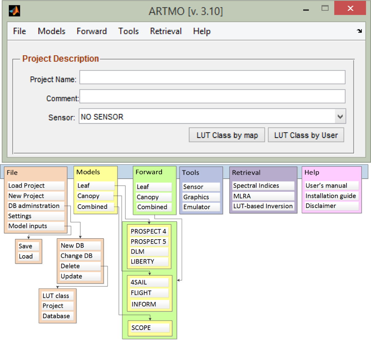
ARTMO brings multiple leaf and canopy radiative transfer models (RTMs) together along with essential tools required for semi-automatic retrieval of biophysical parameters in a modular toolbox. In short, the toolbox permits the user: (1) to choose between various invertible leaf and canopy RTMs of a low to high complexity (e.g., PROSPECT-4, PROSPECT-5, SAIL, FLIGHT, INFORM, SCOPE); in principle any leaf RTM can be coupled with any canopy RTM; (2) to specify or select spectral band settings specifically for various existing air- and space-borne sensors or user-defined settings, typically for recently developed or future sensor systems; (3) to simulate large datasets of top-of-canopy (TOC) reflectance spectra for sensors sensitive in the optical range (400 to 2500 nm); (4) to generate look-up tables (LUT), which are stored in a relational SQL database management system (MySQL, Version 5.5 or higher; local instalment required); and, finally, (5) to configure and run various retrieval scenarios using EO reflectance datasets for biophysical parameter mapping applications. ARTMO is developed in MATLAB (2009 version or higher). Figure 1 presents ARTMO’s (v.3.10) main window and a systematic overview of the drop-down menu below. To start with, in the main window, a new project can be initiated, a sensor chosen and a comment added, whereas all processing modules are accessible through drop-down menus at the top bar.
The first rudimentary version of ARTMO has been used in LUT-based inversion applications [15,31]. The toolbox has been improved and expanded since then, such as by the implementation of retrieval modules. They are based on parametric and non-parametric regression, as well as physically-based inversion using a LUT and led to the development of a: (1) “Spectral Indices assessment toolbox” [37]; (2) “Machine Learning Regression Algorithm (MLRA) toolbox” [57]; and (3) “LUT-based inversion toolbox” [58]. ARTMO v3.10 with the “Emulator toolbox v. 1.00” is formally presented in this paper. The software package is freely downloadable at http://ipl.uv.es/artmo. ARTMO’s general architecture is outlined in Figure 2.
3.1. Emulator Settings Module
The algorithms and architecture of the Emulator toolbox are essentially based on the MLRA toolbox [57]. Similarly to the MLRA toolbox, the first step consists of inserting input data, which refer to the RTM LUT data (input data and associated output spectra). This is done in “Input” and gives the user the possibility to select a predefined LUT as generated by ARTMO. That LUT can be generated for any leaf, canopy or combined RTM and for any optical sensor in the 400- to 2500-nm range. Once the data are linked, the “Settings” module can be configured.
In the “Settings” module, the available MO-MLRA’s (PLSR, NN, KRR) can be configured given various options. One MO-MLRA can be selected or, alternatively, all available MO-MLRAs can be solved one-by-one. In addition, options to add independent white Gaussian noise are provided. Noise can be added to the retrieved parameters or to the spectra. The injection of noise can be important in order to account for environmental and instrumental uncertainties. Fourth, the training/validation data partition can be controlled by setting the percentage of how much data from an RTM or user-defined setting is assigned to training or to validation (i.e., split-sample approach). Thereby, the user can evaluate the impact of ranging training/validation partitioning by entering a range of training/validation partitions. Alternatively, a cross-validation module has been implemented that allows the user to select k-fold or leave-one-out (LOO) cross-validation schemes. Cross-validation returns a more robust estimate of the model’s performance, by averaging statistics from multiple independent training and test subsets. Finally, to enable the models to cope with large, contiguous hyperspectral datasets (e.g., reflectance, fluorescence spectra), the option of applying a principal component analysis (PCA) dimensionality reduction step prior to training a model has been implemented. An emulator on projections is thus generated. In this case, the inverse of the PCA transformation is applied to obtain reconstructed spectra. This dimensionality reduction technique greatly speeds up the training phase, which in case of NNs can take a long time and makes the problem better conditioned.
3.2. Validation Module
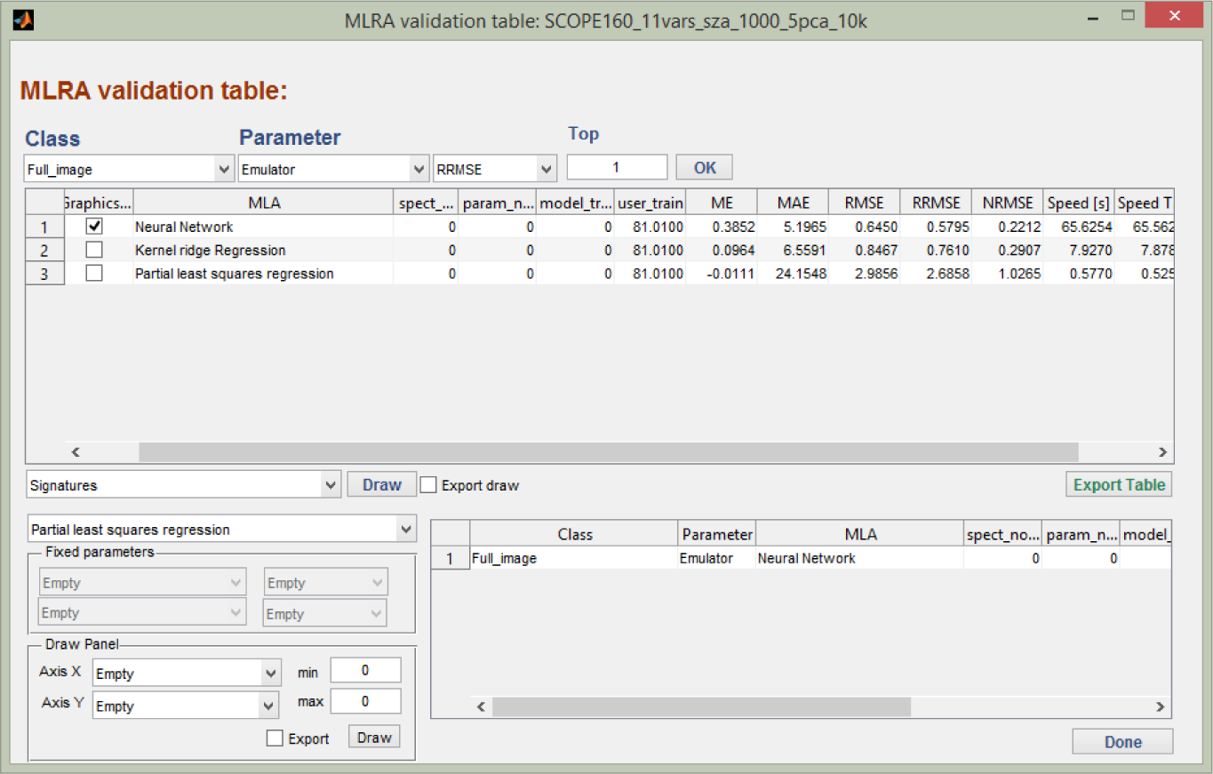
Once the training/validation data splitting have been defined and the settings configured, a range of scenarios can be run, tested and their performance assessed. This is done by naming a validation set in the “Validation” module. Each regression model strategy over the configured ranges are one-by-one analysed through the root-mean-square-error (RMSE) difference between emulated spectra and RTM spectra assigned to validation, and the results are stored in a MySQL database. As such, a large number of results can be stored in a systematic manner, so that they can be easily queried and compared. An example of validation results is presented in the “MLRA validation table” (Figure 3).
The table shows the best performing validation results per model according to RMSE indicators, such as the normalized RMSE (i.e., relative RMSE to the range parameter measurements), further referred to as relative error, and training and validation processing speed. Options to visualize the performance of the emulator are provided, such as displaying the best and worst emulated spectrum relative to their true counterpart or a user-defined emulated and validation spectrum. Finally, by clicking on “Retrieval”, a successfully-validated regression function can be selected to function as the emulator (e.g., the best evaluated MLRA model).
3.3. Emulator Module
The “Emulator module” is the core of the Emulator toolbox. It consists of the following utilities:
Emulator vs. RTM: In the Emulator test interface, the option is provided to configure a random simulation and then run it by the emulator, as well as by the RTM. Subsequently, the RMSE difference between the validation and the emulated spectrum is provided, as well as the processing speed for both. In this way, the accuracy and processing speed of the emulator can be inspected.
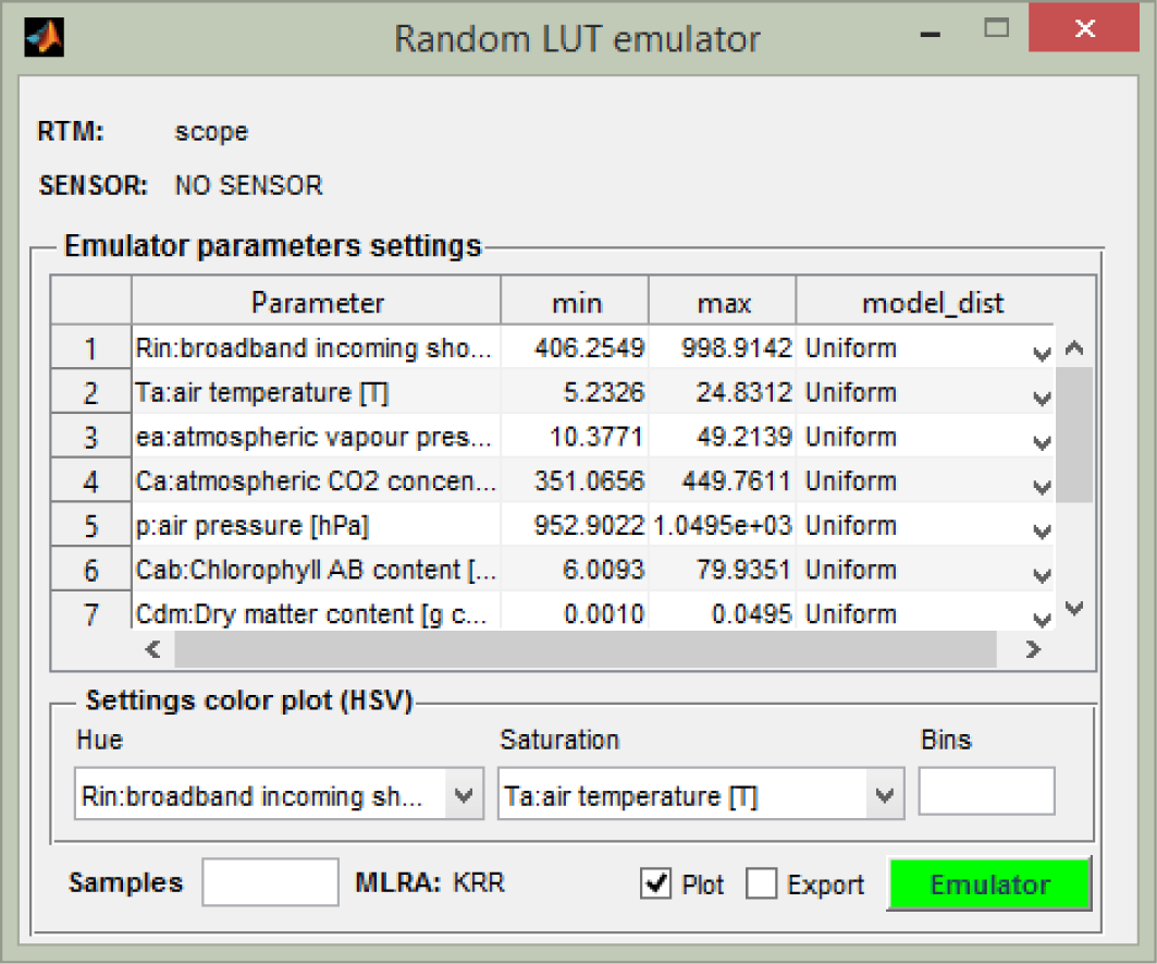
Random LUT Emulator: In the emulator LUT generation interface, a random LUT can be emulated by entering the required input variables, the minimum and maximum boundaries, the sample distribution (e.g., normal, uniform), the number of samples and the directory of the output file. Emulated spectra can be plotted and exported.
User Emulator: Alternatively, the user can also import their own text file with RTM input values. As such, any kind of spectral dataset can be emulated, e.g., input data can come from field measurements, but also from ARTMO-exported input data. Emulated spectra can be plotted and exported.
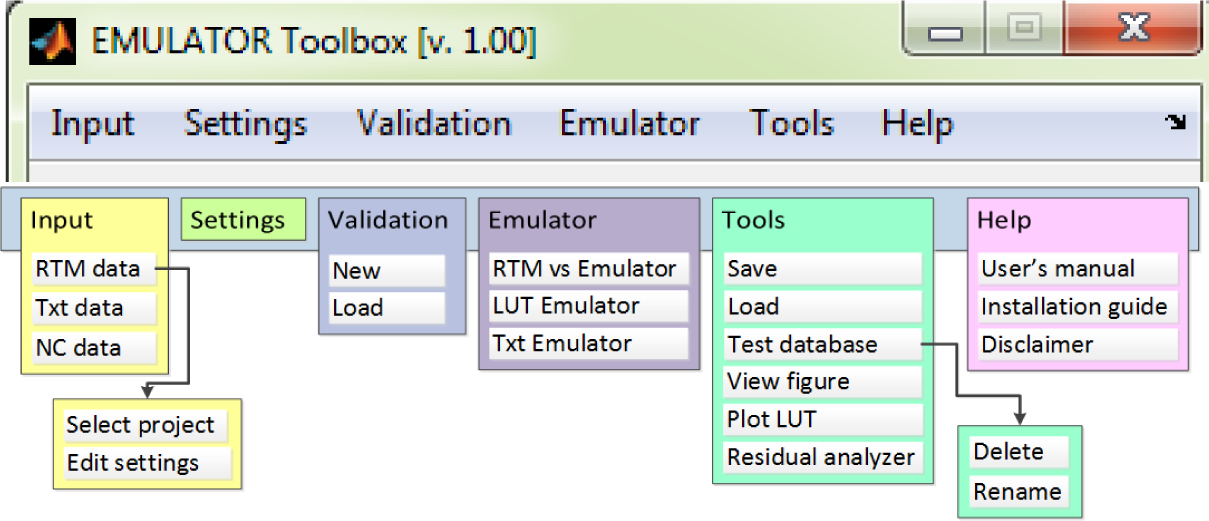
A screen shot of the Random LUT Emulator is shown in Figure 4, and the other utilities are designed in a similar way. Finally, the toolbox offers a few additional tools to inspect the accuracy of the emulators, such as plotting the spectral residuals (i.e., the difference between RTM-generated and emulated-generated spectra in absolute or relative terms) and some general statistics derived from the residuals. Furthermore, the possibility is provided to track back which samples (or bands) caused the best and worst emulated spectra, respectively.
4. Proof of Concept: Emulating Fluorescence Profiles
Having the Emulator toolbox presented, as a proof of concept, we subsequently applied it for evaluating the performance of the three MO-MLRAs on their capability to emulate the SVAT model SCOPE (Soil Canopy Observation, Photochemistry and Energy fluxes) [21]. SCOPE is essentially an energy budget model that calculates the whole energy budget of a canopy, with sun-induced chlorophyll fluorescence as one of the outputs. These simulations are used within FLEX applications, e.g., for the development of artificial scenes as observed by FLEX and for sensitivity studies. Here, we will evaluate whether the emulator reaches acceptable accuracies and how much processing speed is gained. SCOPE is first outlined, followed by the experimental setup of the LUT generation. Emulating results are then presented and discussed.
4.1. Simulated Data: SCOPE v1.60
SCOPE calculates radiation transfer in a multilayer canopy in order to obtain reflectance and fluorescence in the observation direction as a function of the solar zenith angle and leaf inclination distribution. The distribution of absorbed radiation within the canopy is calculated with the SAIL model [33]. The distribution of absorbed radiation is further used in a micro-meteorological representation of the canopy for the calculation of photosynthesis, fluorescence, latent and sensible heat. The fluorescence and thermal radiation emitted by individual leaves is finally propagated through the canopy, again with the SAIL modelling concept [21]. Apart from the canopy radiative transfer modules, the following leaf-level modules are relevant at this point:
A leaf radiative transfer module that calculates absorbed photosynthetically-active radiation (aPAR), reflectance and fluorescence spectra as a function of the irradiance spectrum and the leaf composition;
A biochemical module that calculates the photosynthesis rate and the fraction of absorbed light returning as fluorescence, as a function of aPAR, temperature, relative humidity and the concentrations of CO2 and O2.
Compared to an earlier release [21], various improvements have been included in the new SCOPE v1.60 [59], such as processing speed-up through parallel computing routines. Nevertheless, SCOPE v1.60 still takes about one second to finalize a single simulation. Because SCOPE v1.60 is equipped with over 30 input variables and offers a wide range of output products (organized according to fluxes, radiation, reflectance, spectrum, surface temperature, fluorescence, vertical profiles), all types of input-output sensitivity studies can be conducted. However, this comes at a computational cost. In view of FLEX, we are mostly interested in sun-induced fluorescence (SIF) outputs. We will therefore examine the capability of the MO-MLRAs to emulate SCOPE fluorescence profiles.
4.2. Experimental Setup
Although SCOPE is equipped with over 30 input variables, not all of them play a role in the generation of fluorescence outputs. To find out their relative importance, in an earlier work, a global sensitivity analysis (GSA) was employed [60]. It was found that 11 key variables explained 95.5% of the variance of total SIF(integral of the fluorescence broadband signal). These variables, listed in Table 1, were therefore used to generate SCOPE LUTs.
A fully random LUT within the variable space with minimum and maximum boundaries as given in Table 1 and a uniform distribution was generated using SCOPE v1.60 for 100, 500, 1000 and 5000 samples. Their processing time took 75, 386, 774 and 4177 seconds, respectively. These LUTs were then entered into the Emulator toolbox, with the fluorescence variable as the selected output. Within the “Settings” window, for each LUT, all three MO-MLRAs were selected. In order to speed up the model development, prior to training the MO-MLRAs, a PCA was applied, and the first five components were retained and used for data projection. The impact of applying a PCA with five components as opposed to without using PCA was tested for KRR and 1000 samples. It was found that differences were negligible (∆ RMSE: 0.0004), which suggests that applying PCA can be considered as a valid dimensionality reduction technique. Further, in order to generate more robust validation results, a 10-fold cross-validation sub-sampling procedure was applied. The advantage of using a k-fold cross-validation sampling is that all data are used for both training and validation, and each single observation is used for validation exactly once. The generated RMSE statistics are then averaged over the 10 subsets.
5. Results
5.1. MO-MLRA Evaluation
Table 2 displays the RMSECV goodness-of-fit statistics of the validation dataset and the training and validation processing computational cost of the four MO-MLRAs for the 100, 500, 1000 and 5000 random samples datasets. The normalized RMSE (NRMSECV) indicates that relative errors fall below 3%, but significant differences across the three MO-MLRAs and sampling size can be observed. Regarding the three MO-MLRAs, the PLSR performed poorest in accuracy. NN was validated as best performing for the datasets of 500, 1000 and 5000 samples, closely followed by KRR. For NN and KRR, predictive accuracy improved when more samples are given to the model. With 5000 training samples, relative errors fell below0.3%. KRR and NN are in principle very efficient with less than 5000 samples. However, NN needed significantly more time to train the model because of its complex optimization during the learning process; KRR only requires tuning the kernel length-scale and the regularization parameter, while for NN, we tuned the number of hidden neurons from three to 40, as well as the learning rate, momentum term, regularization constants and initialization of the weights. When introducing many samples (e.g., 5000), KRR starts being computationally demanding, because it requires inverting an increasingly large kernel matrix. Note that the PCA transformation considerably improved the computational efficiency of the training phase; without PCA, it took up to a few hours to develop the NN model. In turn, once trained, all three MO-MLRA models generate emulations quasi-instantly.
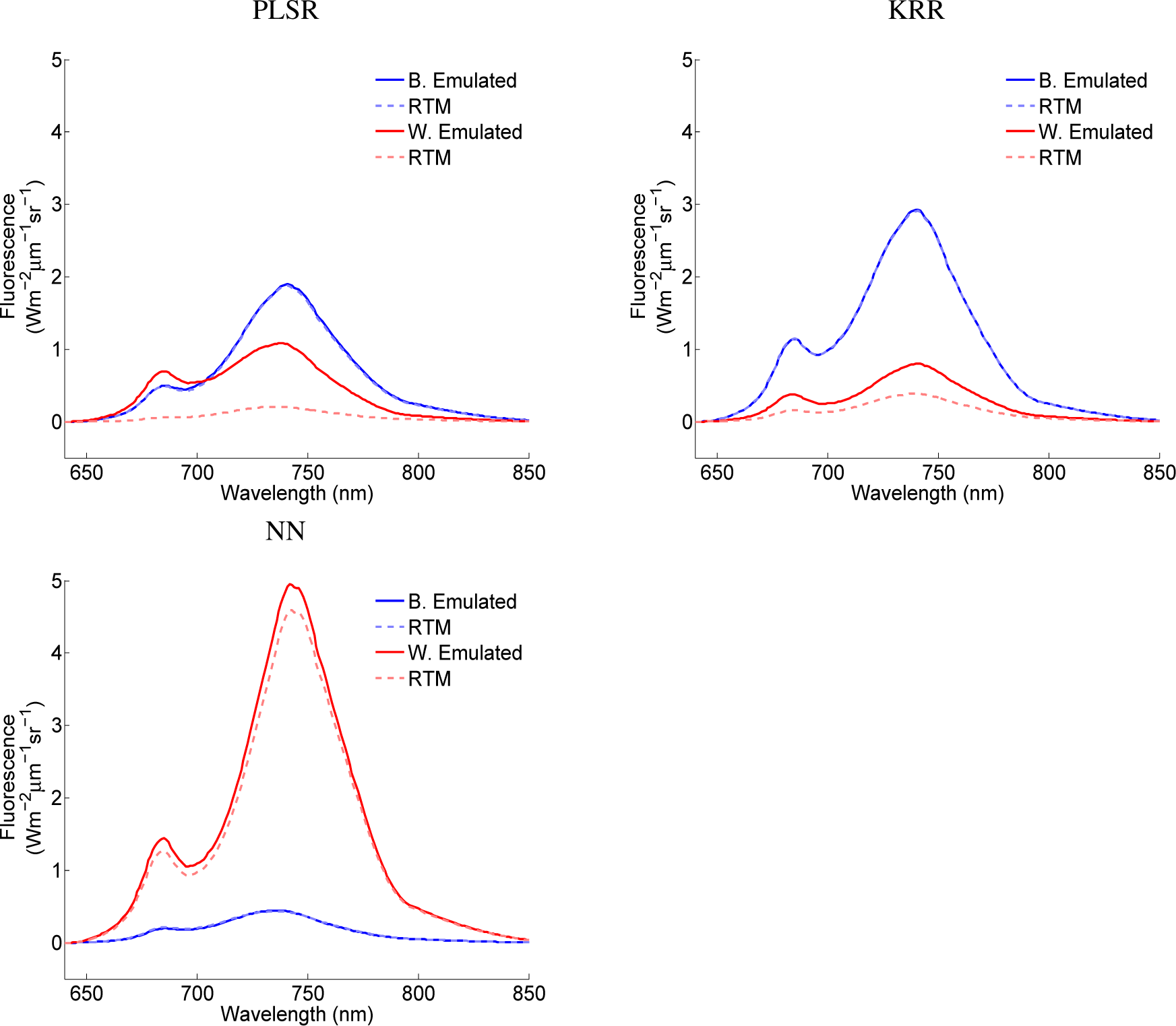
While these goodness-of-fit statistics provided a general indication of the model performance, to visualize the ability of these models to emulate SCOPE fluorescence outputs, the best and worst matching emulation according to the RMS deviation are plotted for the three MO-MLRAs for the case of the 1000 samples (see Figure 5). It can be observed that for each MO-MRLA, the best validated fluorescence profile perfectly matched the original SCOPE profile. Perhaps more interesting is to inspect the worst emulated fluorescence profile. Large differences can be observed in the case of PLSR; it completely missed the close-to-zero fluorescence profile. Furthermore, KRR overestimated a weak fluorescence profile, but considerably less pronounced. Interestingly, for NN, a similar weak fluorescence profile was encountered as the best matching. Here, as the worst match, a slight overestimation occurred for a pronounced fluorescence profile. Considering the close approximation of the SCOPE fluorescence profile, it shows the powerful potential of NN to approximate the physical RT model SCOPE.
The MO-MLRA models were used to generate emulated fluorescence profiles for the input data of the 100, 500, 1000 and 5000 random samples within the Table 1 defined input boundaries. As such, the gain in processing speed can be compared to the original simulations (Table 2, last column). It can be observed that the emulator reconstructs the fluorescence profiles multiple times faster than the original SCOPE RTM. Approximately, NN delivers fluorescence about 50-times faster, PLSR about 400-times faster and KRR even about 400- to 900-times faster (depending on the amount of training data) than the SCOPE model. Hence, given that KRR is several times faster than NN and almost as accurate, it is a promising MO-MLRA to function as an emulator.
5.2. Emulated LUT Evaluation
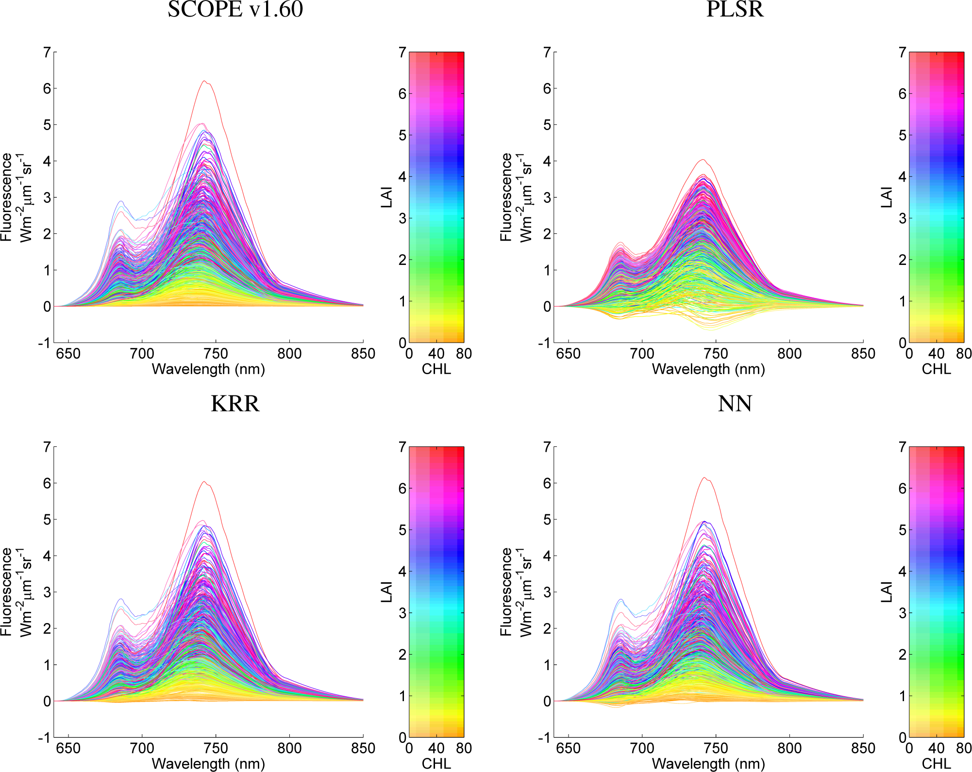
To illustrate the performance of the MO-MLRAs on their ability to reconstruct fluorescence profiles, they are visualized for the 1000 samples in Figure 6. The top-left panel displays the original SCOPE fluorescence profiles; the other panels display the 1000 emulated profiles for the three MO-MLRA models.
Although these profiles were generated by 11 randomly-varying variables, the profiles were colour-plotted as a function of CHL and LAI. With these graphs, it can be observed that PLSR cannot be considered as an accurate emulator; PLSR does not reach the same magnitude as the original SCOPE profiles and, more problematic, leads to negative fluorescence profiles. These effects were actually expected, because PLSR, even being a supervised regression algorithm, can only find orthogonal transforms (rotations) and apply a linear regression model. In turn, KRR and NN delivered much more accurate profiles and can cope with the non-linearities of the problem; they are within the same magnitudes as the original SCOPE profiles; and only a few profiles turn out to fall slightly below zero. For the large majority of samples, KRR and NN reconstructed the 1000 fluorescence spectra with precision.
Considering the few fluorescence profiles that fall below zero, obviously they do not make sense physically. When taking a closer look, it appears these are mostly profiles with a close-to-zero LAI. Hence, this case study underlines that careful inspection of the emulator performance is necessary before applying it to a practical application. For instance, the emulator performs more successfully when emulating well within the training variable space than emulating at or beyond the training boundaries. Accordingly, when setting the LAI boundary to a minimum of 0.5, then no more negative values appeared (results not shown). A similar trend was observed in the case of 5000 samples (results not shown), though with slightly reduced below-zero profiles, due to the somewhat more accurate emulator performance because of being trained by more samples.
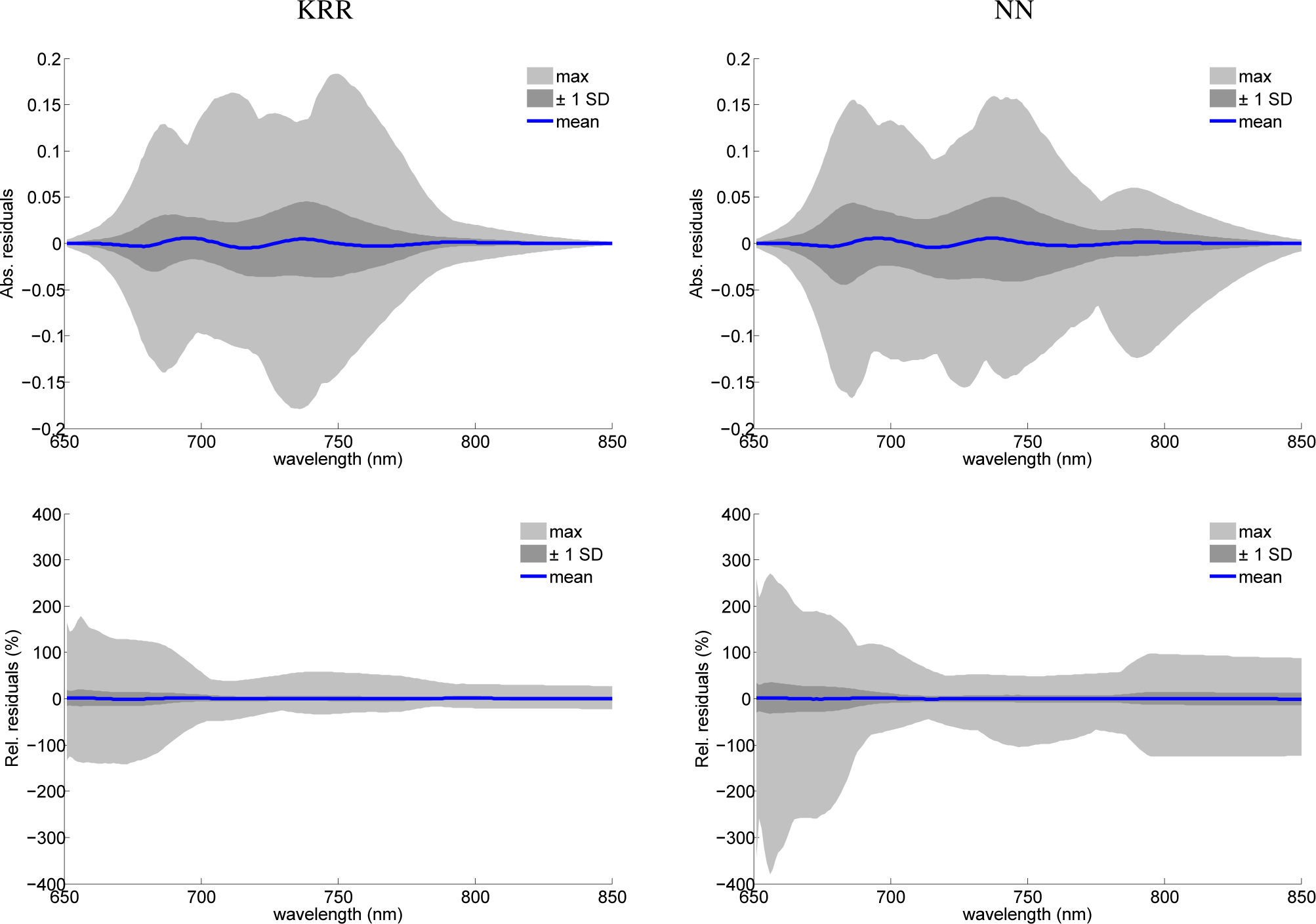
As a final analysis, the spectral residuals between fluorescence spectra and the original SCOPE model and emulated fluorescence spectra of the MO-MLRAs were calculated. To summarize these residuals, some general statistics are provided in Figure 7, i.e., the mean, ±1 standard deviation (SD) and the maximal area covered within the 97.5% percentile. Both absolute as well as relative statistics are shown, but only for KRR and NN. Residuals of PLSR showed a systematic mismatch with a magnitude almost 10-times larger than NN and KRR and, therefore, are not shown. Consequently, PLSR cannot be recommended as a suitable emulator. In turn, KRR and NN show more promising perspectives. The mean of the signatures is close to zero, as well as the ±1 SD, which in absolute terms stayed below 0.05. When inspecting the SD in relative terms, then it can be observed that it stayed below 25% for KRR and below 35% for NN, with a widening at the tails of the fluorescence profiles due to close-to-zero absolute values. Hence, for the large majority of samples, KRR and NN emulators generated accurate fluorescence profiles, with a preference for KRR that performed better in relative terms (bottom plots). Only a few emulated spectra caused outliers with relative errors beyond 50%, especially for NN. When tracking back to the input variables of those poorest 1% residuals, this reveals that these emulated profiles are characterized with input variables of at least one, but mostly a combination of two or more, extreme input values, i.e., reaching the edges of the training variable space. As a rule of thumb, it is recommended to use emulators well within the boundary space, as was presented by the training dataset. With the tools provided by the Emulator toolbox in hand, the user can firstly select the best-performing MO-MLRA model based on RMSE metrics and then inspect its performance with tools “Emulator vs. RTM” or spectral residual analysis.
6. Discussion
Radiative transfer models (RTMs) are widely used in the retrieval of biophysical variables through inversion strategies. Though they are typically restricted to the so-called economically-invertible RTMs, which are characterized by a relatively low number of input variables and being fast in their processing (e.g.,SAIL). Such an approach typically works well over homogeneous landscapes, but the turbid medium model PROSAIL may not be appropriate to process heterogeneous landscapes. For instance, various studies addressing the inversion of PROSAIL faced difficulties when inverting over heterogeneous scenes, such as row crops, heterogeneous grasslands and forests [13,61]. Consequently, these studies typically recommend investing in more advanced RTMs that possess flexibility to interpret heterogeneous scenes. However, that feature implies an increasing number of input variables and computational cost. The difficulty found when inverting more advanced RTMs has been repeatedly acknowledged [23,24]. One of the main drawbacks of advanced RTMs is their long processing time, which impedes the generation of LUTs and inversion strategies and their use in operational processing chains.
To overcome this drawback, based on the idea that RTMs can be substituted through statistical constructs in a computationally-efficient way [25], in this paper, we presented a novel, readily available Emulator toolbox. The toolbox provides the necessary tools to enable emulating advanced RTMs. The core of the toolbox consists of multi-output machine learning regression algorithms (MO-MLRAs) that are able to reconstruct spectral outputs, e.g., radiance, reflectance or fluorescence spectra. As a case study, it was demonstrated that the SVAT model SCOPE can be successfully approximated by an MO-MLRA with high accuracy (relative errors (NRMSECV) below 0.5% when trained with 500 or more samples for KRR and NN) to generate fluorescence outputs. More importantly, the outputs are generated multiple orders of magnitude faster than the physical RTM, with the actual gain in speed depending on the processing time of the RTM and the used MO-MLRA. Here, KRR generated fluorescence spectra at a processing speed about 800-times faster than SCOPE. However, it must be noted that emulators are by no means intended to replace RTMs. After all, RTMs are needed for the training phase, but also, the observation that not in all cases a perfect reconstruction is achieved requires that emulators should be used with caution. Inspection of the performance is a necessity, especially when passing beyond the variables boundaries of what has been presented during the training phase. Further research is necessary to ascertain whether emulators can be applied to any kind of RTM generating a diversity of outputs, e.g., reflectance, radiance, fluorescence, temperature, microwave, etc. Important questions hereby concern the minimum number of training data required to achieve acceptable accuracies, as well the number of input variables the emulator can successfully cope with. With the Emulator toolbox, these questions can be easily investigated, either for RTMs readily available within ARTMO or by means of importing training data (a LUT) as generated by models outside ARTMO.
To pursue this research line further, in the next version, more MO-MLRAs are planned to be implemented within the Emulator toolbox. For instance, the multi-output (MO) version of support vector regression (MO-SVR) [62] or the MO version of random forests (MO-RF) [63] or Gaussian processes regression (MO-GPR) [25]. Particularly the latter is of interest, as MO-GPR possesses the advantage to deliver, apart from estimates, also associated uncertainties. As such, a threshold can be inbuilt that allows one to automatically filter out emulated spectra with high uncertainties. Eventually, more powerful MO-MLRAs may approximate RTMs more accurately than the currently evaluated ones. In this respect, the Emulator toolbox opens opportunities for many new applications. A few examples are listed below:
Opportunities are opened to retrieve biophysical variables through advanced RTMs. By emulating these models, this allows generating of LUTs at the same processing speeds as economically-invertible RTMs. This implies that advanced RTMs can be used in operational processing chains and data assimilation processes.
The ability to generate large LUTs that fill up the full parameter space opens opportunities to conduct global sensitivity analysis (GSA) studies for advanced, computationally-expensive models. This approach has earlier been demonstrated for a SVAT model called SimSphere [20,30]. Accordingly, the same approach can be applied to advanced RTMs. Currently, we are involved in implementing a GSA toolbox in ARTMO.
RTMs are increasingly used as core algorithms of end-to-end simulators (E2Es). An E2ES is a set of algorithms and software tools reproducing the planned mission configuration to assess mission performance; to consolidate technical requirements and system implementation; and to analyse the suitability of the developed retrieval schemes. The basis of an E2E is a scene generation module, where a synthetic scene is generated. This requires a large number of simulations, often with advanced models. For instance, in preparation of the FLEX mission, a scene generator module is under development that consists of the coupling of the SVAT model SCOPE with the atmospheric model MODTRAN [7]. Because of the large processing time of SCOPE and MODTRAN, the possibilities to substitute these models by emulators are currently studied.
7. Conclusions
Emulators are statistical constructs that approximate the functioning of a physically-based radiative transfer model (RTM). They provide great savings in memory and tremendous gains in processing speed, while yielding similar accuracies in reconstructing RTM outputs. This emulating approach opens many new research and operational remote sensing opportunities. To facilitate the use of emulators, ARTMO’s new “Emulator toolbox” currently enables analysing three multi-output machine learning regression algorithms (MO-MLRAs), both linear (partial least squares regression (PLSR)) and non-linear (kernel ridge regression (KRR), neural networks (NN)). The toolbox enables the user to train the MO-MLRA models with data coming from RTMs that are available within ARTMO. Various options are provided that can optimize the training phase, such a PCA pre-processing step, ranging training/validation distributions or through cross-validation sub-sampling procedures. The goodness-of-fit performance and processing speed of the MO-MLRAs are then calculated. A successfully-validated MO-MLRA can then function as an emulator.
As a proof of concept, we analysed the ability of the implemented MO-MLRAs to substitute the SVAT model SCOPE in the generation of fluorescence outputs. Although PLSR cannot be considered as an accurate emulator, NN and KRR emulated fluorescence profiles with great precision (relative errors below 0.5% when trained with 500 or more samples), and this with a gain in processing speed of about 50 (NN) up to about 800 (KRR) times faster than SCOPE v1.60. It is foreseen that the Emulator toolbox will open up a diverse range of new applications using advanced RTMs, such as improved inversion strategies, global sensitivity analysis studies and rendering of simulated scenes in preparation for new satellite missions.
Acknowledgments
This paper has been partially supported by ESA’s “FLEX-Bridge Study” (ESA ESTEC Contract No. 4000112341/14/NL/FF/gp). We thank the authors of the RTMs and MO-MLRAs for making their codes publicly available to the ARTMO toolbox. We also thank three reviewers for their valuable suggestions.
Author Contributions
Juan Pablo Rivera developed the toolbox presented here and contributed to executing the experiments. The co-authors of this manuscript significantly contributed to all phases of the investigation: Jochem Verrelst supervised the research project, developed this paper’s study concept, performed the experiments and wrote the paper. Jose Gómez-Dans developed the Emulator concept, and Jordi Muñoz-Marí and Gustau Camps-Valls contributed to the machine learning sections and manuscript editing. José Moreno contributed to manuscript editing.
Conflicts of Interest
The authors declare no conflict of interest.
References
- Widlowski, J.L.; Taberner, M.; Pinty, B.; Bruniquel-Pinel, V.; Disney, M.; Fernandes, R.; Gastellu-Etchegorry, J.P.; Gobron, N.; Kuusk, A.; Lavergne, T.; et al. Third Radiation Transfer Model Intercomparison (RAMI) exercise: Documenting progress in canopy reflectance models. J. Geophys. Res. Atmos. 2007, 112, D09111. [Google Scholar]
- Baret, F.; Buis, S. Estimating canopy characteristics from remote sensing observations. Review of methods and associated problems. In Advances in Land Remote Sensing: System, Modeling, Inversion and Application; Liang, S., Ed.; Springer: New York, NY, USA, 2008; pp. 171–200. [Google Scholar]
- Jacquemoud, S.; Verhoef, W.; Baret, F.; Bacour, C.; Zarco-Tejada, P.; Asner, G.; François, C.; Ustin, S. PROSPECT + SAIL models: A review of use for vegetation characterization. Remote Sens. Environ. 2009, 113, S56–S66. [Google Scholar]
- Verrelst, J.; Camps Valls, G.; Muñoz Marí, J.; Rivera, J.; Veroustraete, F.; Clevers, J.; Moreno, J. Optical remote sensing and the retrieval of terrestrial vegetation bio-geophysical properties—A review. ISPRS J. Photogramm. Remote Sens. 2015. in press. [Google Scholar]
- Verhoef, W.; Bach, H. Simulation of Sentinel-3 images by four-stream surface-atmosphere radiative transfer modelling in the optical and thermal domains. Remote Sens. Environ. 2012, 120, 197–207. [Google Scholar]
- Segl, K.; Guanter, L.; Rogass, C.; Kuester, T.; Roessner, S.; Kaufmann, H.; Sang, B.; Mogulsky, V.; Hofer, S. EeteSThe EnMAP end-to-end simulation tool. IEEE J. Select. Top. Appl. Earth Obs. Remote Sens. 2012, 5, 522–530. [Google Scholar]
- Rivera, J.; Sabater, N.; Tenjo, J.; Vicent, N.; Alonso, L. Moreno. Synthetic scene simulator for hyperspectral spaceborne passive optical sensors. In Application to ESA’s FLEX/Sentinel-3 Tandem Mission; WHISPERS, IEEE: Lausanne, Switzerland, 2014. [Google Scholar]
- Widlowski, J.L.; Pinty, B.; Lopatka, M.; Atzberger, C.; Buzica, D.; Chelle, M.; Disney, M.; Gastellu-Etchegorry, J.P.; Gerboles, M.; Gobron, N.; et al. The fourth radiation transfer model intercomparison (RAMI-IV): Proficiency testing of canopy reflectance models with ISO-13528. J. Geophys. Res. Atmos. 2013, 118, 6869–6890. [Google Scholar]
- Knyazikhin, Y.; Kranigk, J.; Myneni, R.; Panfyorov, O.; Gravenhorst, G. Influence of small-scale structure on radiative transfer and photosynthesis in vegetation canopies. J. Geophys. Res. D Atmos. 1998, 103, 6133–6144. [Google Scholar]
- Atzberger, C.; Richter, K. Spatially constrained inversion of radiative transfer models for improved LAI mapping from future Sentinel-2 imagery. Remote Sens. Environ. 2012, 120, 208–218. [Google Scholar]
- Weiss, M.; Baret, F. Evaluation of canopy biophysical variable retrieval performances from the accumulation of large swath satellite data. Remote Sens. Environ. 1999, 70, 293–306. [Google Scholar]
- Combal, B.; Baret, F.; Weiss, M.; Trubuil, A.; Macé, D.; Pragnère, A.; Myneni, R.; Knyazikhin, Y.; Wang, L. Retrieval of canopy biophysical variables from bidirectional reflectance using prior information to solve the ill-posed inverse problem. Remote Sens. Environ. 2003, 84, 1–15. [Google Scholar]
- Darvishzadeh, R.; Skidmore, A.; Schlerf, M.; Atzberger, C. Inversion of a radiative transfer model for estimating vegetation LAI and chlorophyll in a heterogeneous grassland. Remote Sens. Environ. 2008, 112, 2592–2604. [Google Scholar]
- Houborg, R.; Anderson, M.; Daughtry, C. Utility of an image-based canopy reflectance modelling tool for remote estimation of LAI and leaf chlorophyll content at the field scale. Remote Sens. Environ. 2009, 113, 259–274. [Google Scholar]
- Verrelst, J.; Rivera, J.; Leonenko, G.; Alonso, L.; Moreno, J. Optimizing LUT-based RTM inversion for semiautomatic mapping of crop biophysical parameters from Sentinel-2 and -3 data: Role of cost functions. IEEE Trans. Geosci. Remote Sens. 2014, 52, 257–269. [Google Scholar]
- Govaerts, Y.M.; Verstraete, M.M. Raytran: a monte carlo raytracing model to compute light scattering in threedimensional heterogeneous media. IEEE Trans. Geosci. Remote Sens. 1996, 36, 493–305. [Google Scholar]
- North, P. Three-dimensional forest light interaction model using a Monte Carlo method. IEEE Trans. Geosci. Remote Sens. 1996, 34, 946–956. [Google Scholar]
- Disney, M.; Lewis, P.; North, P. Monte Carlo ray tracing in optical canopy reflectance modelling. Remote Sens. Rev. 2000, 18, 163–196. [Google Scholar]
- Gastellu-Etchegorry, J.; Demarez, V.; Pinel, V.; Zagolski, F. Modeling radiative transfer in heterogeneous 3-D vegetation canopies. Remote Sens. Environ. 1996, 58, 131–156. [Google Scholar]
- Petropoulos, G.; Wooster, M.; Carlson, T.; Kennedy, M.; Scholze, M. A global Bayesian sensitivity analysis of the 1d SimSphere soil-vegetation-atmospheric transfer (SVAT) model using Gaussian model emulation. Ecol. Model. 2009, 220, 2427–2440. [Google Scholar]
- Van Der Tol, C.; Verhoef, W.; Timmermans, J.; Verhoef, A.; Su, Z. An integrated model of soil-canopy spectral radiances, photosynthesis, fluorescence, temperature and energy balance. Biogeosciences 2009, 6, 3109–3129. [Google Scholar]
- Demarez, V.; Gastellu-Etchegorry, J. A modelling approach for studying forest chlorophyll content. Remote Sens. Environ. 2000, 71, 226–238. [Google Scholar]
- Gastellu-Etchegorry, J.; Gascon, F.; Esteve, P. An interpolation procedure for generalizing a look-up table inversion method. Remote Sens. Environ. 2003, 87, 55–71. [Google Scholar]
- Malenovsky, Z.; Martin, E.; Homolova, L.; Gastellu-Etchegorry, J.P.; Zurita-Milla, R.; Schaepman, M.; Pokorna, R.; Clevers, J.; Cudlin, P. Influence of woody elements of a Norway spruce canopy on nadir reflectance simulated by the DART model at very high spatial resolution. Remote Sens. Environ. 2008, 112, 1–18. [Google Scholar]
- Gómez-Dans, J.L.; Lewis, P.E. Efficient emulation of radiative transfer models using Gaussian processes 2015. in press.
- Lewis, P.; Gómez-Dans, J.; Kaminski, T.; Settle, J.; Quaife, T.; Gobron, N.; Styles, J.; Berger, M. An Earth Observation Land Data Assimilation System (EO-LDAS). Remote Sens. Environ. 2012, 120, 219–235. [Google Scholar]
- Rasmussen, C.E.; Williams, C.K.I. Gaussian Processes for Machine Learning; The MIT Press: New York, NY, USA, 2006. [Google Scholar]
- Kennedy, M.; O’Hagan, A. Predicting the output from a complex computer code when fast approximations are available. Biometrika 2000, 87, 1–13. [Google Scholar]
- Kennedy, M.; O’Hagan, A. Bayesian calibration of computer models. J. R. Stat. Soc. Ser. B Stat. Methodol. 2001, 63, 425–450. [Google Scholar]
- Ireland, G.; Petropoulos, G.; Carlson, T.; Purdy, S. Addressing the ability of a land biosphere model to predict key biophysical vegetation characterisation parameters with global sensitivity analysis. Environ. Model. Softw. 2015, 65, 94–107. [Google Scholar]
- Verrelst, J.; Romijn, E.; Kooistra, L. Mapping vegetation density in a heterogeneous river floodplain ecosystem using pointable CHRIS/PROBA data. Remote Sens. 2012, 4, 2866–2889. [Google Scholar]
- Feret, J.B.; François, C.; Asner, G.P.; Gitelson, A.A.; Martin, R.E.; Bidel, L.P.R.; Ustin, S.L.; le Maire, G.; Jacquemoud, S. PROSPECT-4 and 5: Advances in the leaf optical properties model separating photosynthetic pigments. Remote Sens. Environ. 2008, 112, 3030–3043. [Google Scholar]
- Verhoef, W. Light scattering by leaf layers with application to canopy reflectance modelling: The SAIL model. Remote Sens. Environ. 1984, 16, 125–141. [Google Scholar]
- Atzberger, C. Development of an invertible forest reflectance model: The INFOR-model, Proceedings of the 20th EARSeL Symposium, Dresden, Germany, 14–16 June 2000; pp. 39–44.
- O’Hagan, A. Bayesian analysis of computer code outputs: A tutorial. Reliab. Eng. Syst. Saf. 2006, 91, 1290–1300. [Google Scholar]
- Verrelst, J.; Muñoz, J.; Alonso, L.; Delegido, J.; Rivera, J.; Camps-Valls, G.; Moreno, J. Machine learning regression algorithms for biophysical parameter retrieval: Opportunities for Sentinel-2 and -3. Remote Sens. Environ. 2012, 118, 127–139. [Google Scholar]
- Rivera, J.; Verrelst, J.; Delegido, J.; Veroustraete, F.; Moreno, J. On the semi-automatic retrieval of biophysical parameters based on spectral index optimization. Remote Sens. 2014, 6, 4924–4951. [Google Scholar]
- Arenas-García, J.; Petersen, K.B.; Camps-Valls, G.; Hansen, L.K. Kernel multivariate analysis framework for supervised subspace learning. IEEE Signal Proc. Mag. 2013, 30, 16–29. [Google Scholar]
- Jolliffe, I.T. Principal Component Analysis; Springer-Verlag: Berlin, Germany; New York, NY, USA, 1986. [Google Scholar]
- Wold, H. Partial least squares. Encycl. Stat. Sci. 1985, 6, 581–591. [Google Scholar]
- Geladi, P.; Kowalski, B. Partial least-squares regression: A tutorial. Anal. Chim. Acta 1986, 185, 1–17. [Google Scholar]
- Coops, N.C.; Smith, M.L.; Martin, M.; Ollinger, S.V. Prediction of eucalypt foliage nitrogen content from satellite-derived hyperspectral data. IEEE Trans. Geosci. Remote Sens. 2003, 41, 1338–1346. [Google Scholar]
- Gianelle, D.; Guastella, F.b. Nadir and off-nadir hyperspectral field data: Strengths and limitations in estimating grassland biophysical characteristics. Int. J. Remote Sens. 2007, 28, 1547–1560. [Google Scholar]
- Cho, M.B.; Skidmore, A.B.; Corsi, F.; van Wieren, S.; Sobhan, I.B. Estimation of green grass/herb biomass from airborne hyperspectral imagery using spectral indices and partial least squares regression. Int. J. Appl. Earth Obs. Geoinform. 2007, 9, 414–424. [Google Scholar]
- Ye, X.; Sakai, K.; Manago, M.; Asada, S.I.; Sasao, A. Prediction of citrus yield from airborne hyperspectral imagery. Precis. Agric. 2007, 8, 111–125. [Google Scholar]
- Haykin, S. Neural Networks—A Comprehensive Foundation, 2nd ed.; Prentice Hall: Upper Saddle River, NJ, USA, 1999. [Google Scholar]
- Smith, J. LAI inversion using backpropagation neural network trained with multiple scattering model. IEEE Trans. Geosc. Rem. Sens 1993, 31, 1102–1106. [Google Scholar]
- Gopal, S.; Woodcock, C. Remote sensing of forest change using artificial neural networks. IEEE Trans. Geosci. Remote Sens. 1996, 34, 398–404. [Google Scholar]
- Kimes, D.S.; Nelson, R.F.; Manry, M.T.; Fung, A.K. Attributes of neural networks for extracting continuous vegetation variables from optical and radar measurements. Int. J. Remote Sens. 1998, 19, 2639–2662. [Google Scholar]
- Bacour, C.; Baret, F.; Béal, D.; Weiss, M.; Pavageau, K. Neural network estimation of LAI, fAPAR, fCover and LAI× Cab, from top of canopy MERIS reflectance data: Principles and validation. Remote Sens. Environ. 2006, 105, 313–325. [Google Scholar]
- Verger, A.; Baret, F.; Camacho, F. Optimal modalities for radiative transfer-neural network estimation of canopy biophysical characteristics: Evaluation over an agricultural area with CHRIS/PROBA observations. Remote Sens. Environ. 2011, 115, 415–426. [Google Scholar]
- Baret, F.; Weiss, M.; Lacaze, R.; Camacho, F.; Makhmara, H.; Pacholcyzk, P.; Smets, B. GEOV1: LAI and FAPAR essential climate variables and FCOVER global time series capitalizing over existing products. Part1: Principles of development and production. Remote Sens. Environ. 2013, 137, 299–309. [Google Scholar]
- Shawe-Taylor, J.; Cristianini, N. Kernel Methods for Pattern Analysis; Cambridge University Press: New York, NY, USA, 2004. [Google Scholar]
- Camps-Valls, G., Bruzzone, L., Eds.; Kernel Methods for Remote Sensing Data Analysis; Wiley & Sons: Chichester, UK, 2009.
- Camps-Valls, G.; Muñoz-Marí, J.; Gómez-Chova, L.; Guanter, L.; Calbet, X. Nonlinear statistical retrieval of atmospheric profiles from MetOp-IASI and MTG-IRS infrared sounding data. IEEE Trans. Geosci. Remote Sens. 2012, 50, 1759–1769. [Google Scholar]
- Camps-Valls, G.; Gómez-Chova, L.; Muñoz-Marí, J.; Lázaro-Gredilla, M.; Verrelst, J. simpleR: A Simple Educational Matlab Toolbox for Statistical Regression, V2.1., 2013, Available online: http://www.uv.es/gcamps/code/simpleR.html accessed on 20 April 2015.
- Rivera Caicedo, J.; Verrelst, J.; Muñoz-Marí, J.; Moreno, J.; Camps-Valls, G. Toward a semiautomatic machine learning retrieval of biophysical parameters. IEEE J. Select. Top. Appl. Earth Obs. Remote Sens. 2014, 7, 1249–1259. [Google Scholar]
- Rivera, J.; Verrelst, J.; Leonenko, G.; Moreno, J. Multiple cost functions and regularization options for improved retrieval of leaf chlorophyll content and LAI through inversion of the PROSAIL model. Remote Sens. 2013, 5, 3280–3304. [Google Scholar]
- Van der Tol, C.; Berry, J.A.; Campbell, P.K.E.; Rascher, U. Models of fluorescence and photosynthesis for interpreting measurements of solar-induced chlorophyll fluorescence. J. Geophys. Res. Biogeosci. 2014, 119, 2312–2327. [Google Scholar]
- Verrelst, J.; Rivera, J.; van der Tol, C.; Federico, M.; Mohammed, G.; Moreno, J. Global sensitivity analys of the SCOPE model: What drives simulated canopy-leaving sun-induced fluorescence? Remote Sens. Environ. 2015, 166, 8–21. [Google Scholar]
- Richter, K.; Hank, T.; Vuolo, F.; Mauser, W.; D’Urso, G. Optimal exploitation of the Sentinel-2 spectral capabilities for crop leaf area index mapping. Remote Sens. 2012, 4, 561–582. [Google Scholar]
- Tuia, D.; Verrelst, J.; Alonso, L.; Pérez-Cruz, F.; Camps-Valls, G. Multioutput support vector regression for remote sensing Biophysical parameter estimation. IEEE Geosci. Remote Sens. Lett. 2011, 8, 804–808. [Google Scholar]
- Breiman, L. Random forests. Mach. Learn. 2001, 45, 5–32. [Google Scholar]


| Variable Names | Units | Range | |
|---|---|---|---|
| Leaf biochemistry | |||
| Vcmo | Maximum carboxylation capacity | µmol m−1 s−1 | 0.1 to 100 |
| Leaf variables | |||
| CHL | Leaf chlorophyll content | µg/cm2 | 0 to 80 |
| Cm | Leaf dry matter content | g/cm2 | 0.001 to 0.05 |
| Canopy variables | |||
| LAI | Leaf area index | m2/m2 | 0.01 to 7 |
| rwc | Within-canopy-layer resistance | m2/m2 | 0 to 20 |
| SZA | Solar zenith angle | ○ | 0 to 60 |
| Micrometeorology variables | |||
| Ca | CO2 concentration in the air | ppm | 350 to 450 |
| P | Air pressure | hPa | 1000 to 1090 |
| ea | Atmospheric vapour pressure | hPa | 10 to 50 |
| Ta | Air temperature | °C | 5 to 25 |
| Rin | Incoming shortwave radiation | W m−2 | 400 to 1000 |
| MO-MLRA | RMSECV | NRMSECV (%) | Speed Training (s) | Speed Validation (s) | Gain in Speed (x) |
|---|---|---|---|---|---|
| # 100 | |||||
| PLSR | 3.38 | 2.94 | 0.08 | 0.00 | 312 |
| KRR | 2.29 | 1.32 | 0.07 | 0.01 | 937 |
| NN | 3.91 | 2.37 | 5.50 | 0.05 | 47 |
| # 500 | |||||
| PLSR | 2.92 | 1.16 | 0.23 | 0.01 | 439 |
| KRR | 1.21 | 0.48 | 1.01 | 0.02 | 821 |
| NN | 1.04 | 0.41 | 17.63 | 0.04 | 50 |
| # 1000 | |||||
| PLSR | 2.99 | 1.03 | 0.58 | 0.05 | 423 |
| KRR | 0.85 | 0.29 | 7.88 | 0.05 | 790 |
| NN | 0.64 | 0.22 | 65.56 | 0.06 | 51 |
| # 5000 | |||||
| PLSR | 2.99 | 0.91 | 1.94 | 0.13 | 350 |
| KRR | 0.44 | 0.13 | 435.25 | 0.85 | 411 |
| NN | 0.42 | 0.13 | 486.24 | 0.11 | 54 |
© 2015 by the authors; licensee MDPI, Basel, Switzerland This article is an open access article distributed under the terms and conditions of the Creative Commons Attribution license (http://creativecommons.org/licenses/by/4.0/).
Share and Cite
Rivera, J.P.; Verrelst, J.; Gómez-Dans, J.; Muñoz-Marí, J.; Moreno, J.; Camps-Valls, G. An Emulator Toolbox to Approximate Radiative Transfer Models with Statistical Learning. Remote Sens. 2015, 7, 9347-9370. https://doi.org/10.3390/rs70709347
Rivera JP, Verrelst J, Gómez-Dans J, Muñoz-Marí J, Moreno J, Camps-Valls G. An Emulator Toolbox to Approximate Radiative Transfer Models with Statistical Learning. Remote Sensing. 2015; 7(7):9347-9370. https://doi.org/10.3390/rs70709347
Chicago/Turabian StyleRivera, Juan Pablo, Jochem Verrelst, Jose Gómez-Dans, Jordi Muñoz-Marí, José Moreno, and Gustau Camps-Valls. 2015. "An Emulator Toolbox to Approximate Radiative Transfer Models with Statistical Learning" Remote Sensing 7, no. 7: 9347-9370. https://doi.org/10.3390/rs70709347
APA StyleRivera, J. P., Verrelst, J., Gómez-Dans, J., Muñoz-Marí, J., Moreno, J., & Camps-Valls, G. (2015). An Emulator Toolbox to Approximate Radiative Transfer Models with Statistical Learning. Remote Sensing, 7(7), 9347-9370. https://doi.org/10.3390/rs70709347