In this section, I will compare six different pansharpening methods (see
Section 3.1) and several parameter settings using the proposed JQM and already known QNR joint quality measures, and additionally well-established spectral measures SAM and ERGAS. First, the interpolation influence is only investigated by comparing the four most popular interpolation methods (
Section 3.2). Second, the interpolation method influence on one of the pansharpening methods is analyzed in
Section 3.3. Finally, the comparison of various pansharpening methods and their parameter settings is presented in
Section 3.4.
3.1. Pansharpening Methods
Methods investigated in this paper can be described by the following general expression (see e.g., [
1,
19,
20])
where
msfk—fused/pansharpened high resolution multispectral image,
k—spectral band number,
msik—low resolution multispectral image interpolated to a high resolution space,
gk—weight (gain) for detail injection,
pan—high resolution panchromatic image and
panlpf—low pass filtered
pan image. Usually histogram matching of
msfk and
msk is performed after application of Equation (12). Then, individual methods can be seen as special cases of Equation (12) as shown below.
General Fusion Filtering (GFF) [
21] is defined as
where
gk = 1,
msk—low resolution multispectral image,
ZP—zero padding interpolation,
W—Hamming window for ringing artifacts suppression and
LPF—low pass filter in Fourier domain.
High Pass Filtering Method HPFM (variant of GFF) [
22] is given by
with
gk = 1,
panlpf =
pan*lpf, lpf =
FFT−1(
LPF), where
lpf is a Gaussian low pass filter in signal domain. Here, I have to note that the cutoff frequency of a low pass filter can be selected individually for each spectral band as, e.g., already proposed for MRA based methods using modulation transfer function (MTF) information [
23].
Ehlers fusion [
24] is defined as
where
gk = 1, intensity is defined as
wk are spectral weights calculated from spectral response functions of data provider [
17]. Two different low pass filters are used for filtering of
pan and intensity images, respectively. Usually original software of the method is not available, thus the author’s software implementation is used.
Á trous wavelet transform ATWT [
25] is given by Equation (12) with
gk = 1 and
panlpf—à trous wavelet decomposed low resolution version of
pan. M. Canty’s software implementation [
26] is used.
Component substitution using IHS transformation (CS IHS) can be written as follows
with
gk = 1,
panlpf =
Imsi, and
Imsi is defined by Equation (16). The author’s software implementation is used. Here, I have to note that QHR = 1 for this method what contradicts not to the already known high spatial quality of this method. Thus, usage of an additional measure, e.g., QLR or JQM will allow correctly to discriminate it from other pansharpening methods.
Component substitution using GS transformation (CS GS) is Equation (12) with panlpf = Imsi. IDL ENVI 5.0 software implementation is used.
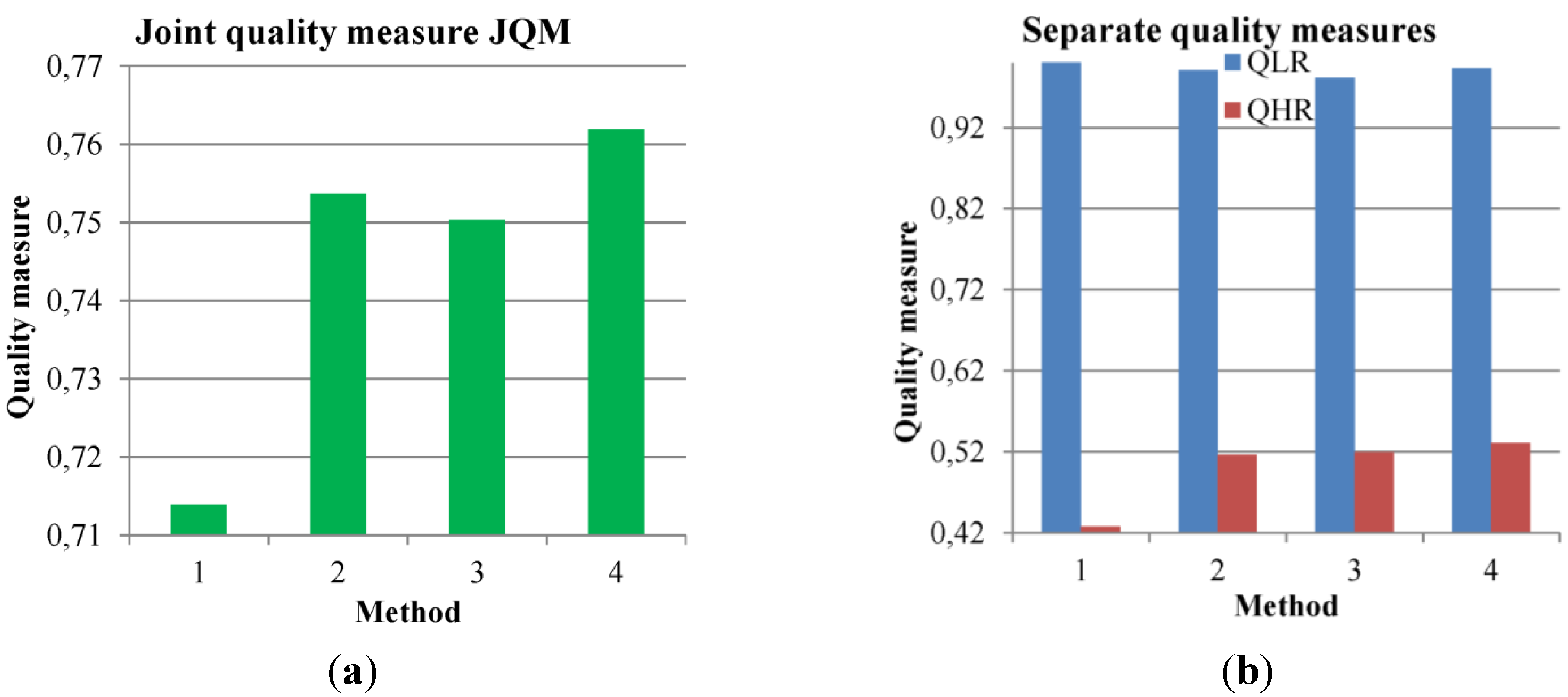
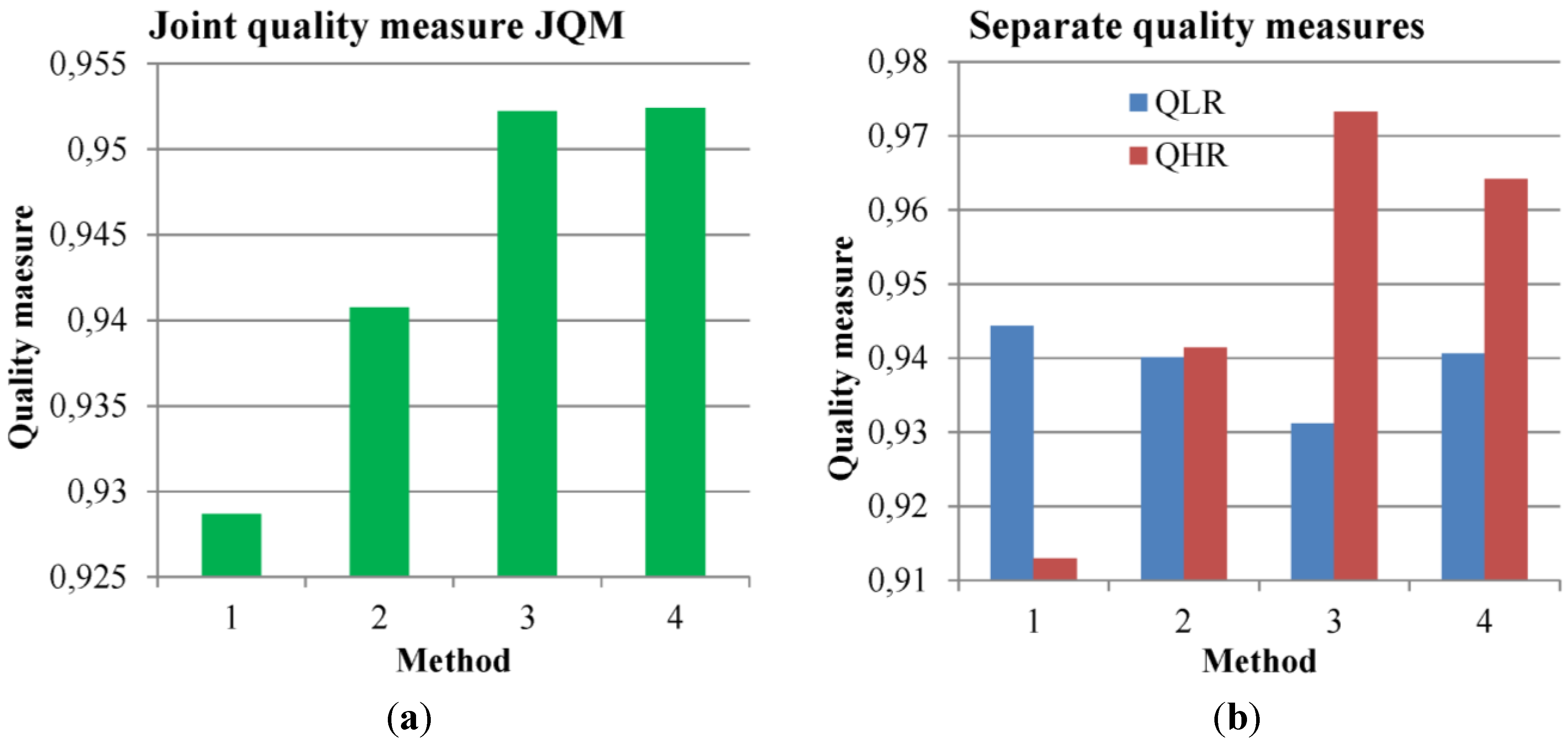
3.2. Interpolation Influence Only
Values of both joint quality measures JQM and QNR and their corresponding separate measures (QLR, QHR and DL, DS) are presented in
Figure 1,
Figure 2,
Figure 3 and
Figure 4 for differently interpolated multispectral data (high resolution scale) of IKONOS (
Figure 1 and
Figure 2) and WV-2 sensors (
Figure 3 and
Figure 4). The following interpolation methods are investigated: nearest neighbor (NN), zero padding using Fourier transform (ZP), bilinear interpolation (BIL) and cubic convolution (CUB) (IDL ENVI 5.0 software is used except ZP, which is the author’s software implementation).
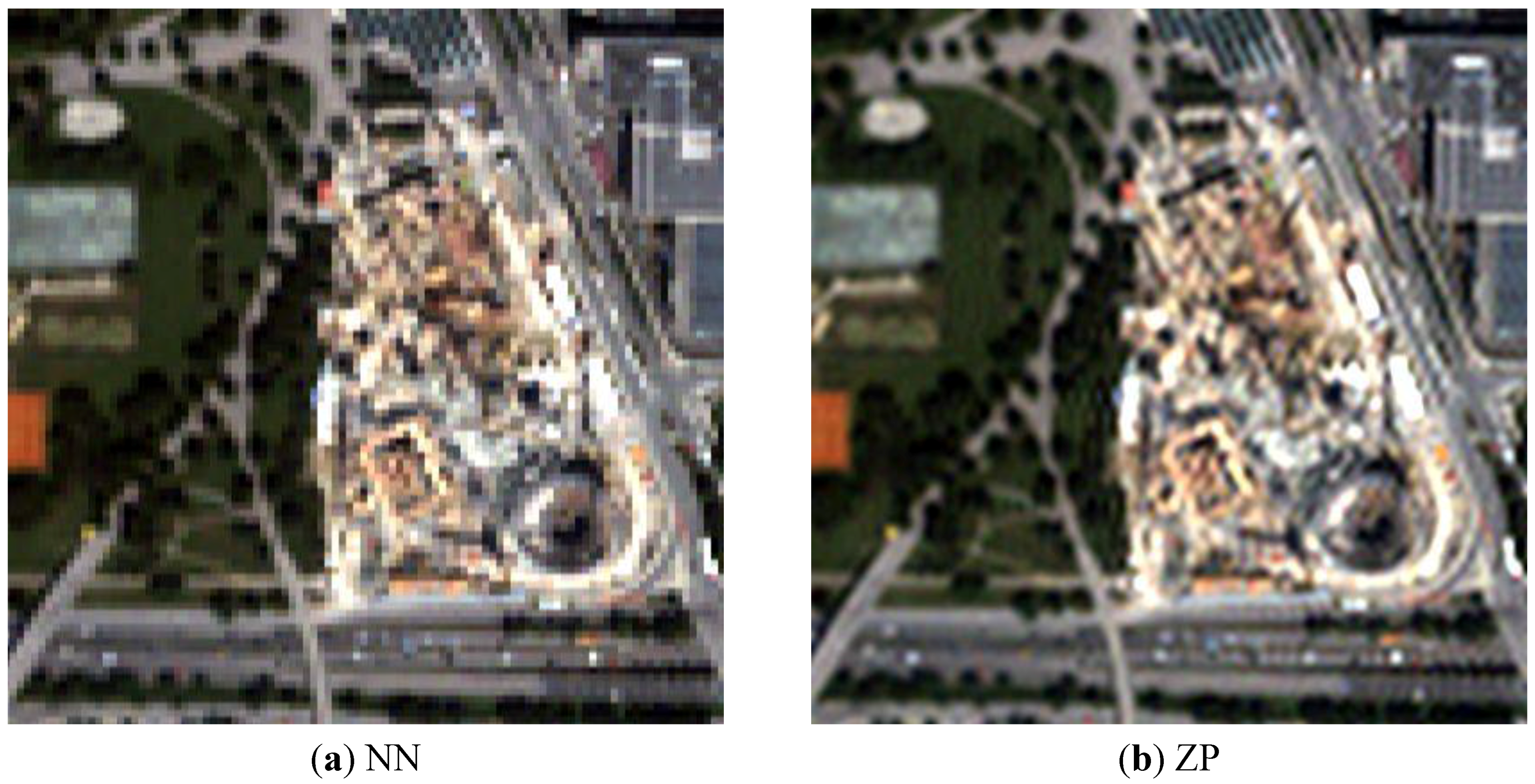
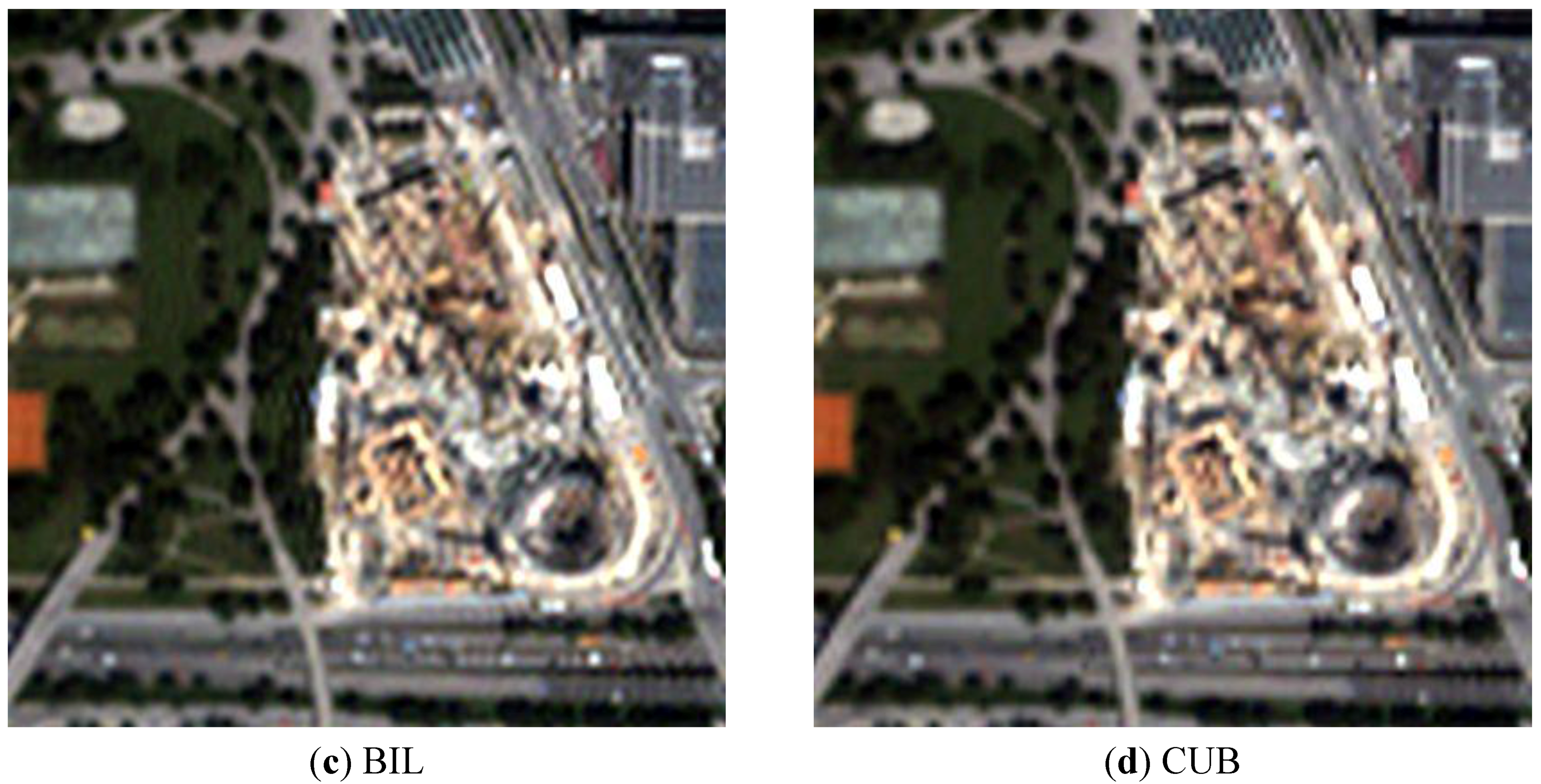
We see that all interpolation methods exhibit quite similar QLR values for both sensors (
Figure 1b and
Figure 3b). For example, this is well supported by visual analysis of interpolation results presented in
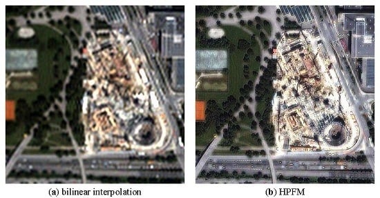
Figure 5. All methods exhibit similar colors or multispectral information. Similarly, all methods have quite similar QHR values except NN. NN has very poor spatial quality. This can be observed in
Figure 5a. These results lead to low (poor) values of JQM for NN for both sensors (
Figure 1a and
Figure 3a). Moderately oscillating values of separate measures QLR and QHR for the other three methods result in slightly higher values of CUB for IKONOS (
Figure 1a) and ZP for WV-2 (
Figure 3a).
Figure 1.
Joint Quality Measure (JQM) quality assessment of interpolation methods: 1—nearest neighbor (NN), 2—zero padding (ZP), 3—bilinear interpolation (BIL), and 4—cubic convolution (CUB) for IKONOS data. (a) JQM, (b) QLR and QHR.
Figure 1.
Joint Quality Measure (JQM) quality assessment of interpolation methods: 1—nearest neighbor (NN), 2—zero padding (ZP), 3—bilinear interpolation (BIL), and 4—cubic convolution (CUB) for IKONOS data. (a) JQM, (b) QLR and QHR.
Figure 2.
Quality with no Reference (QNR) quality assessment of interpolation methods: 1—NN, 2—ZP, 3—BIL, and 4—CUB for IKONOS data. (a) QNR, (b) 1−DL and 1−DS.
Figure 2.
Quality with no Reference (QNR) quality assessment of interpolation methods: 1—NN, 2—ZP, 3—BIL, and 4—CUB for IKONOS data. (a) QNR, (b) 1−DL and 1−DS.
Figure 3.
JQM quality assessment of interpolation methods: 1—NN, 2—ZP, 3—BIL, and 4—CUB for WV-2 data. (a) JQM, (b) QLR and QHR.
Figure 3.
JQM quality assessment of interpolation methods: 1—NN, 2—ZP, 3—BIL, and 4—CUB for WV-2 data. (a) JQM, (b) QLR and QHR.
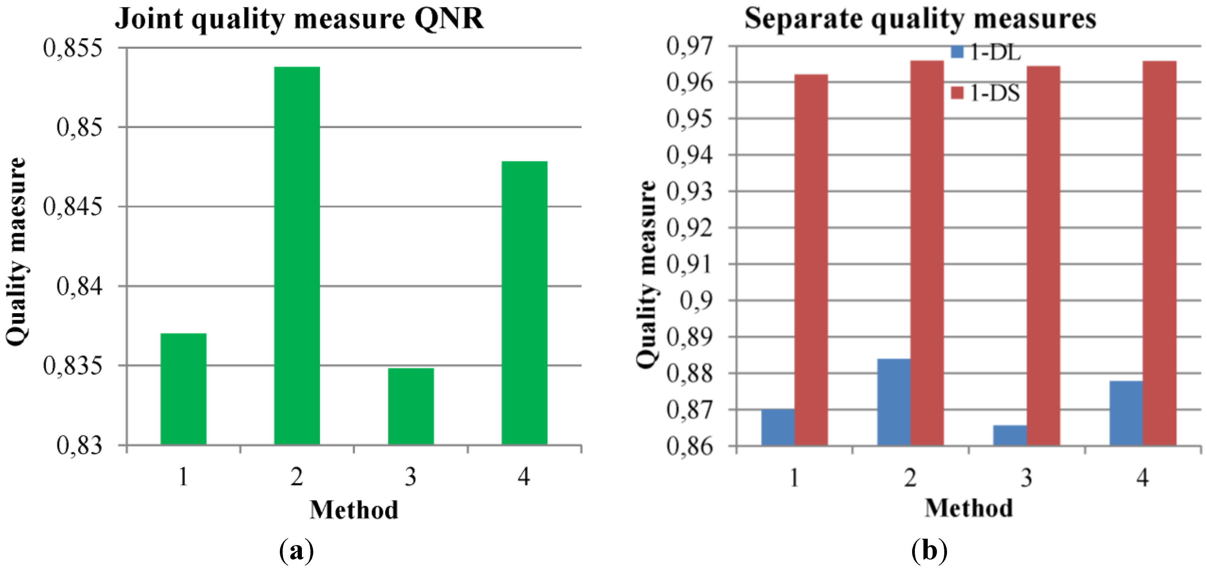
The analysis of QNR is more complex due to greater variability of its compound parts. 1−
DL measure identifies ZP to result in the highest quality, closely followed by CUB. BIL and NN seem to be the worst. Both observations are valid for both sensors (
Figure 2b,
Figure 4b). 1−
DS measure (
Figure 2b) behaves similarly to QLR (
Figure 1b) for IKONOS sensor, but for WV-2 all methods (NN too) seem to be quite similar (
Figure 4b). Moreover, the absolute values of this measure are much higher for WV-2 data than for IKONOS. Thus, the QNR value follows approximately the results of separate measure 1−
DL for both sensors, finally underestimating the BIL method. Similarity of NN and BIL contradicts the visual analysis (
Figure 5). Using QNR it was found that NN as the worst method corresponds quite well to the JQM in this case.
In total it seems that both joint quality measures behave quite similarly except that QNR (1−DL) tends to underestimate BIL interpolation quality. Moreover, 1−DL measure appears to be more sensitive (exhibits higher variability) and 1−DS tends to be dependent on the sensor type.
Figure 4.
QNR quality assessment of interpolation methods: 1—NN, 2—ZP, 3—BIL, and 4—CUB for WV-2 data. (a) QNR, (b) 1−DL and 1−DS.
Figure 4.
QNR quality assessment of interpolation methods: 1—NN, 2—ZP, 3—BIL, and 4—CUB for WV-2 data. (a) QNR, (b) 1−DL and 1−DS.
Figure 5.
Different interpolation methods: NN (a), ZP (b), BIL (c) and CUB (d) for the IKONOS data.
Figure 5.
Different interpolation methods: NN (a), ZP (b), BIL (c) and CUB (d) for the IKONOS data.
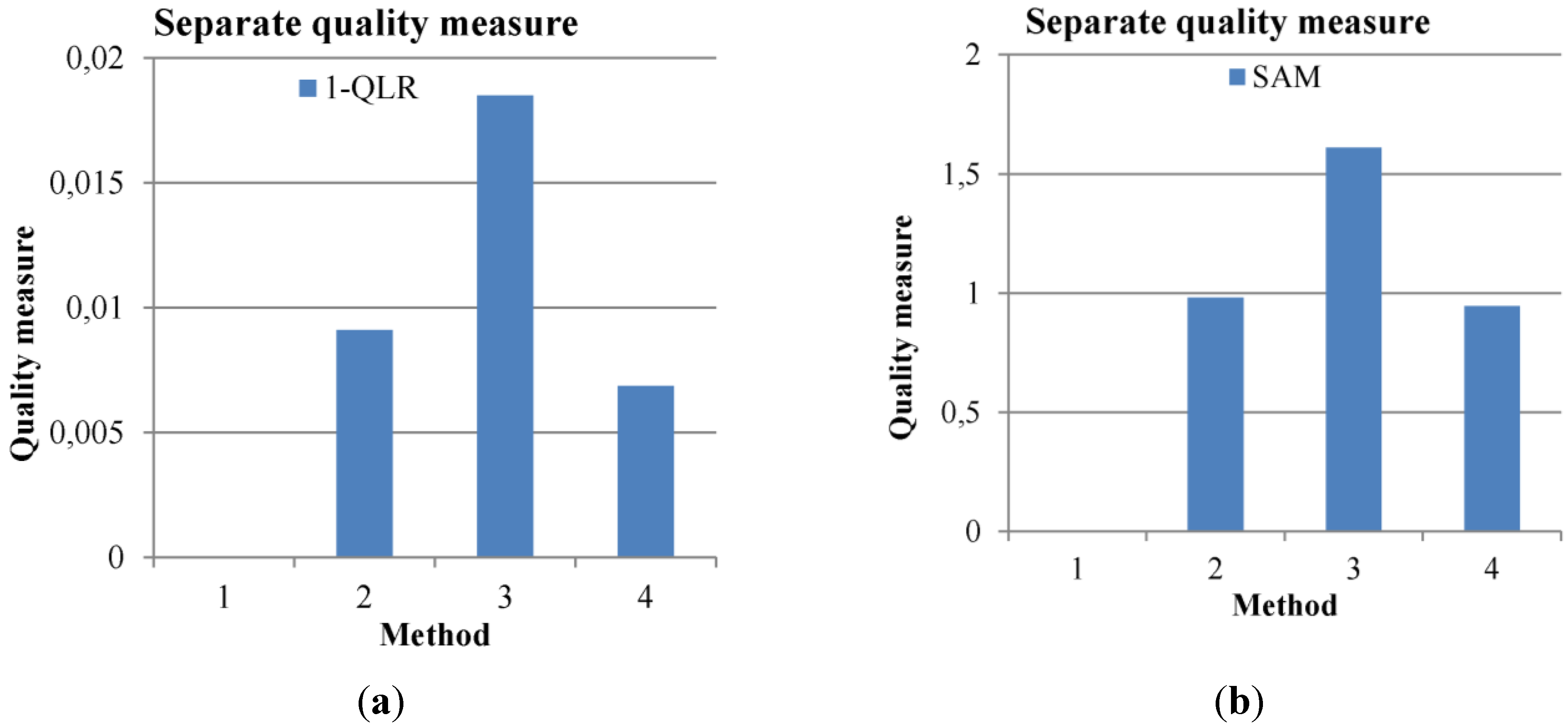
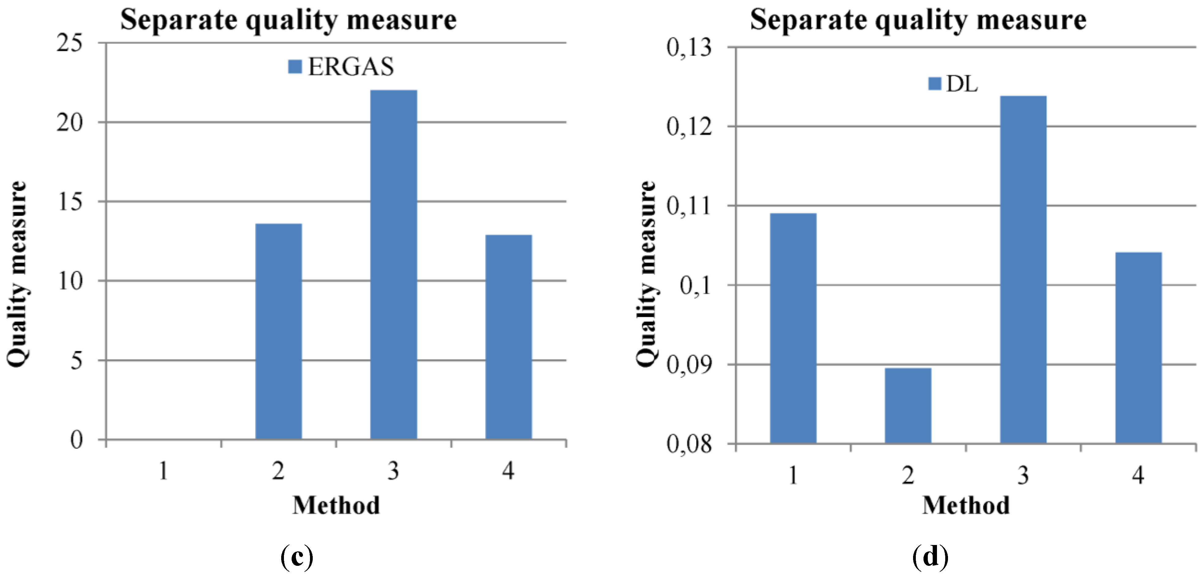
To enhance previously presented experiment, the separate quality measures 1−QLR and
DL are additionally compared with two well established quality measures SAM (given in degrees) and ERGAS in
Figure 6 for IKONOS data. Here, the low measure values stand for similar images. One can see that all measures, except
DL, correlate quite well with each other (
Figure 6a–c). Thus, a new measure QLR is legitimated for a practical usage in pansharpening quality assessment. The
DL measure behaves unexpectedly for NN and ZP by underestimating the quality of NN and overestimating ZP. The reason for that can be the violation of the assumption about the preservation of between-band relations in different resolution scales. Similar results are observed for other experiments of this paper and sensor WV-2 data.
Figure 6.
Quality assessment of interpolation methods: 1—NN, 2—ZP, 3—BIL, and 4—CUB for IKONOS data using different separate quality measures. (a) 1−QLR, (b) SAM, (c) ERGAS, (d) DL.
Figure 6.
Quality assessment of interpolation methods: 1—NN, 2—ZP, 3—BIL, and 4—CUB for IKONOS data using different separate quality measures. (a) 1−QLR, (b) SAM, (c) ERGAS, (d) DL.
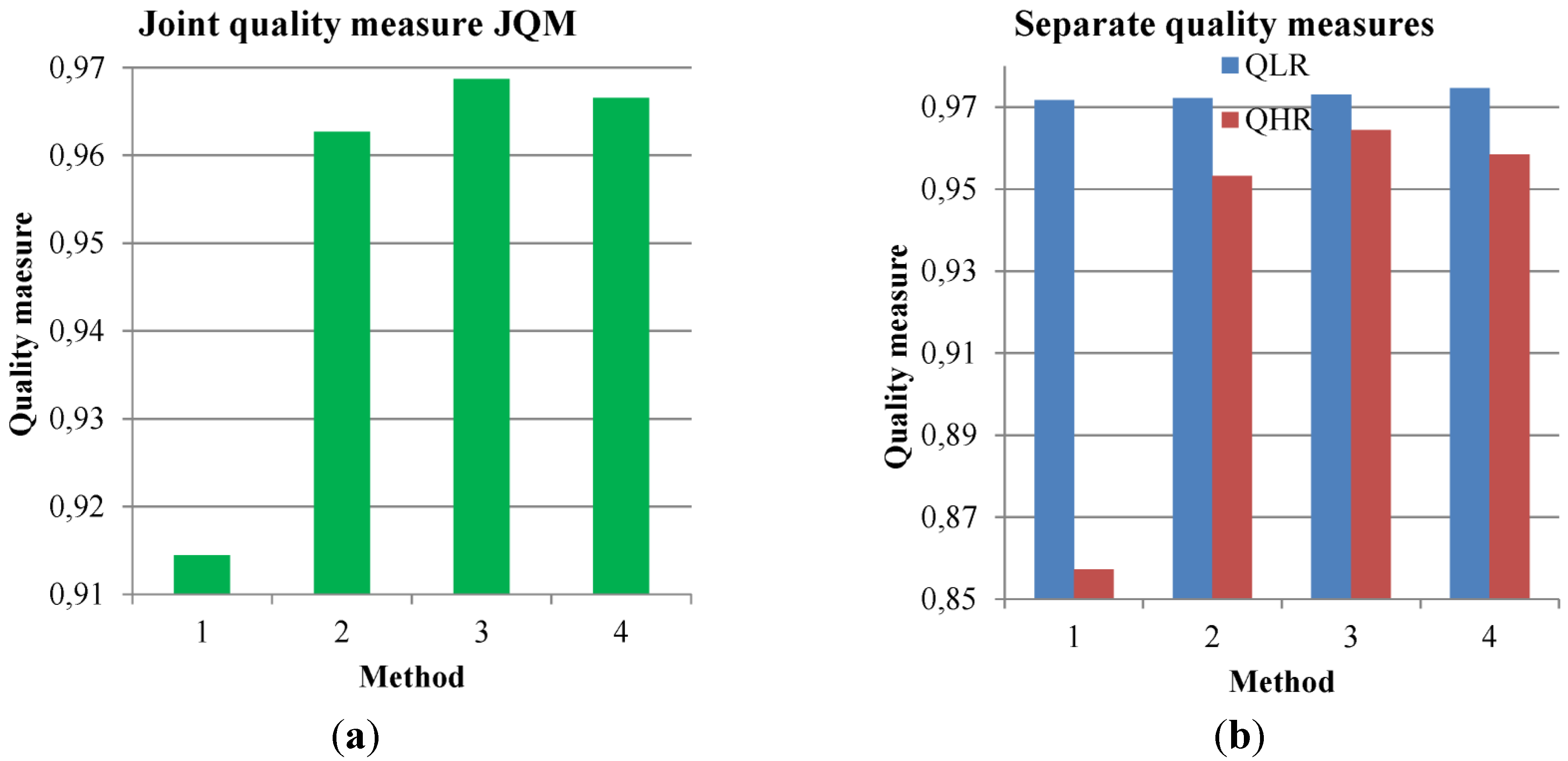
3.3. Interpolation Influence on the HPFM Pansharpening Method
The JQM quality of a selected pansharpening method using different interpolation methods is shown in
Figure 7 and
Figure 8. In this case, the HPFM with a cutoff frequency 0.15 for IKONOS and WV-2 data is used.
Figure 7.
JQM quality assessment of High Pass Filtering Method (HPFM) for different interpolation methods: 1—NN, 2—ZP, 3—BIL, and 4—CUB for IKONOS data. (a) JQM, (b) QLR and QHR.
Figure 7.
JQM quality assessment of High Pass Filtering Method (HPFM) for different interpolation methods: 1—NN, 2—ZP, 3—BIL, and 4—CUB for IKONOS data. (a) JQM, (b) QLR and QHR.
Figure 8.
JQM quality assessment of HPFM for different interpolation methods: 1—NN, 2—ZP, 3—BIL, and 4—CUB for WorldView-2 data. (a) JQM, (b) QLR and QHR.
Figure 8.
JQM quality assessment of HPFM for different interpolation methods: 1—NN, 2—ZP, 3—BIL, and 4—CUB for WorldView-2 data. (a) JQM, (b) QLR and QHR.
QLR is varying insignificantly for IKONOS (
Figure 7b) and almost constant for WV-2 (
Figure 8b) for all interpolation methods. From the point of view of QHR, NN is the worst method and BIL is better than the remaining two methods. These results lead to JQM (
Figure 7a,
Figure 8a) ranking BIL as the best interpolation method for both sensors closely followed by CUB. NN is the worst of all interpolation methods. Thus, it seems that BIL is a suitable interpolation method regardless of sensor type and therefore only BIL interpolation is used in further experiments. The GFF method by definition only uses ZP interpolation method. For Ehlers fusion method, I have followed the recommendation to use CUB [
24]. In ATWT implementation of [
26], NN is used.
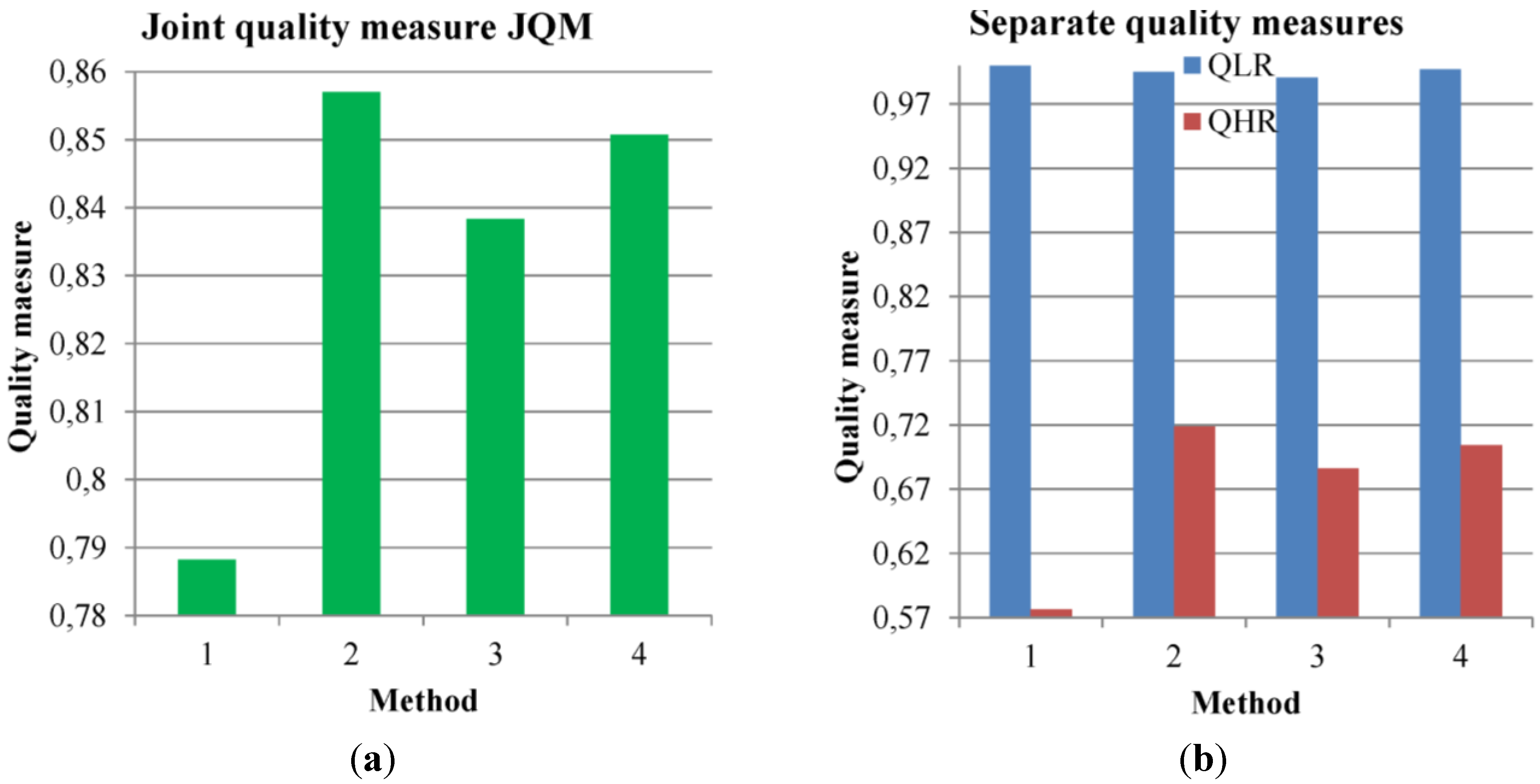
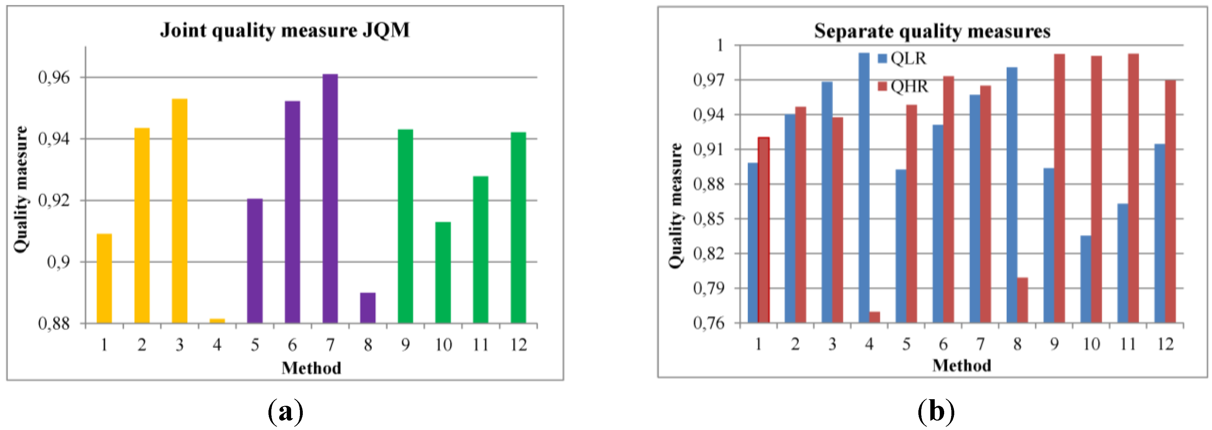
3.4. Comparison of Pansharpening Methods
The pansharpening methods and their parameter settings are listed in
Table 2 ([
21,
22,
24,
25,
26]), and the quantitative comparison results are presented in
Figure 9 and
Figure 10.
Table 2.
List of pansharpening methods.
Table 2.
List of pansharpening methods.
| Method | Cutoff Frequencies | Interpolation Method | Reference |
|---|
| 1 GFF | 0.05 | ZP | [21] |
| 2 GFF | 0.15 | ZP | [21] |
| 3 GFF | 0.3, 0.25, 0.25, 0.15 | ZP | [21] |
| 4 GFF | 0.7 | ZP | [21] |
| 5 HPFM | 0.05 | BIL | [22] |
| 6 HPFM | 0.15 | BIL | [22] |
| 7 HPFM | 0.3, 0.25, 0.25, 0.1 | BIL | [22] |
| 8 HPFM | 0.7 | BIL | [22] |
| 9 CS IHS | - | BIL | - |
| 10 CS GS | - | BIL | IDL ENVI 5.0 |
| 11 ATWT | - | NN | [25,26] |
| 12 Ehlers | 0.15, 0.15 | CUB | [24] |
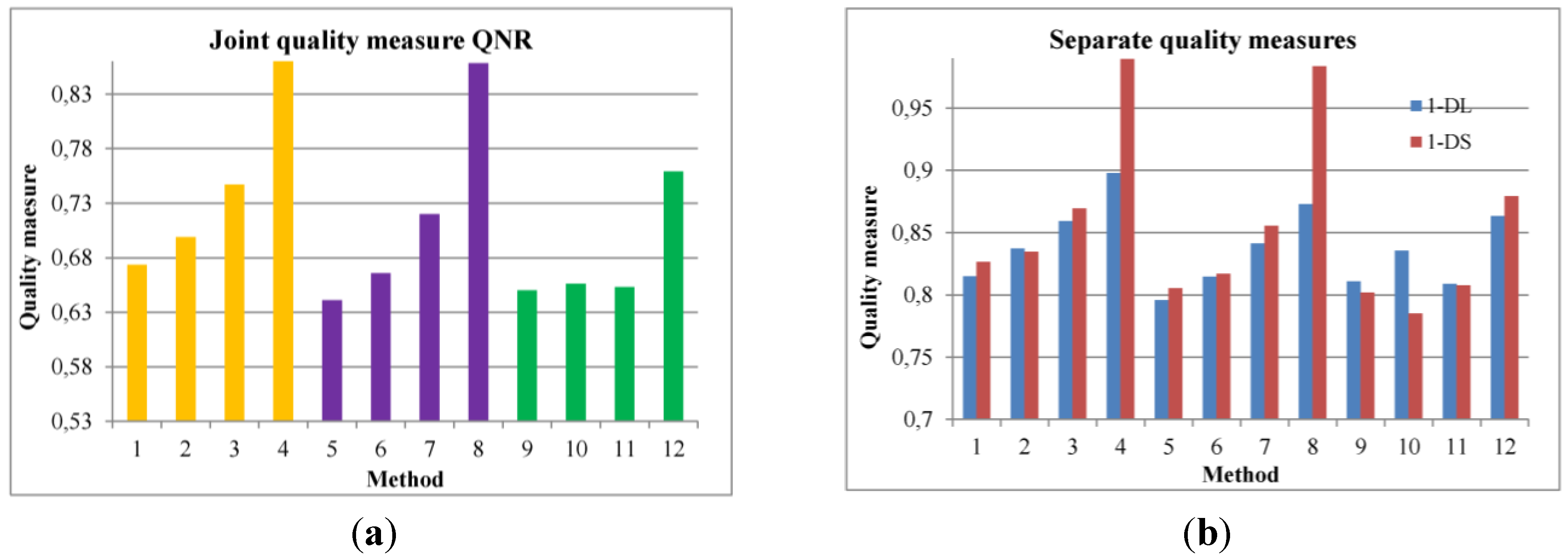
The QLR measure behaves as expected for GFF (methods 1–4) and HPFM (methods 5–8) in dependence of the cutoff frequencies (
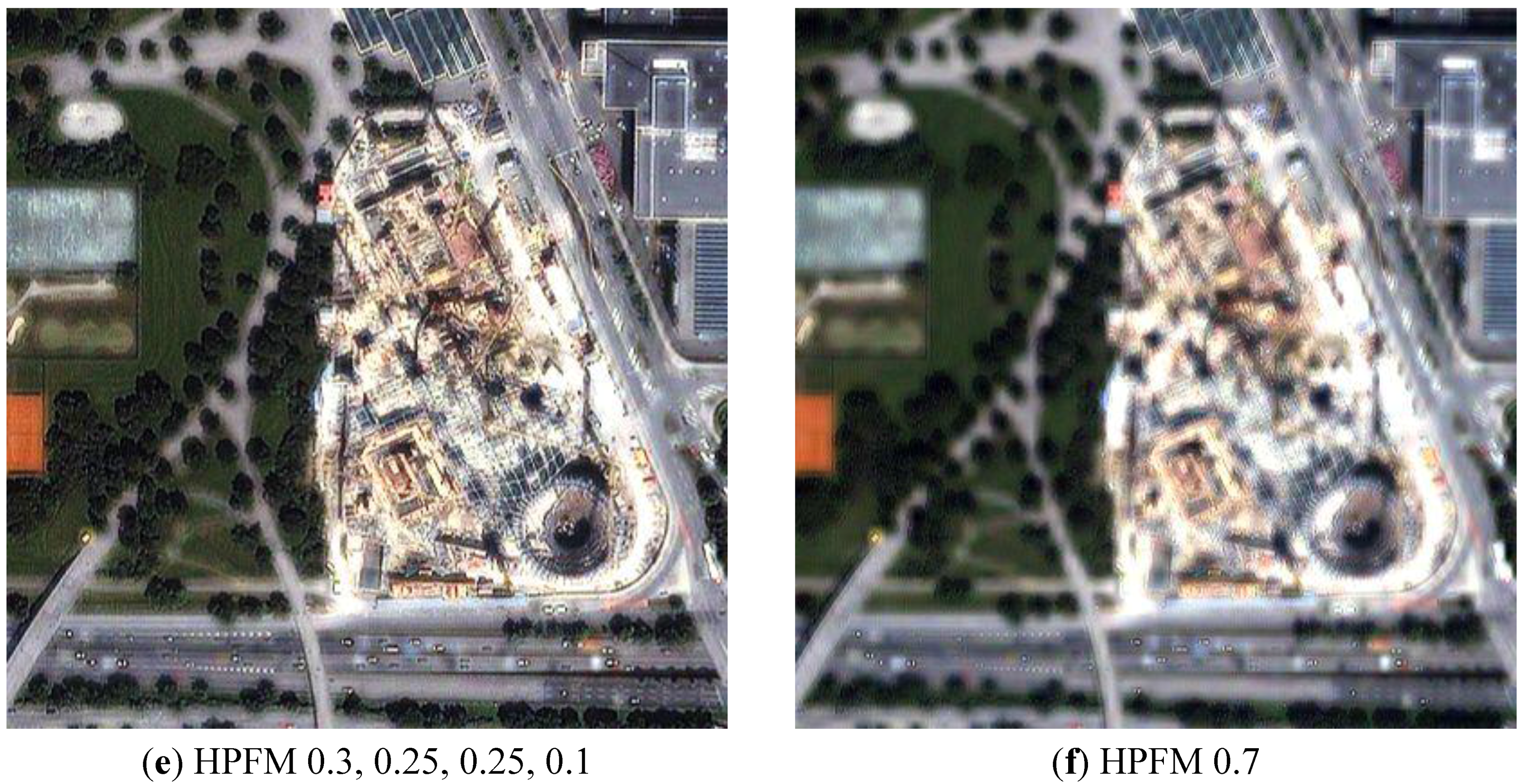
Figure 9b). That is, QLR increases with the increase of cutoff frequency (spectral quality). QHR identifies methods 2 and 6 as the best, which correspond quite well with visual analysis in
Figure 11d. For example, the image in
Figure 11d exhibits much better spatial quality than the image in
Figure 11f. Further, JQM selects methods 3 and 7 with band dependent cutoff frequencies (
Figure 9a), which is well supported by visual interpretation in
Figure 11. For example, the image in
Figure 11e exhibits better spectral quality (e.g., compare with BIL in
Figure 11a) than the image in
Figure 11d simultaneously preserving good spatial quality. Moreover, it seems that HPFM, the faster variant of GFF, is better than GFF, maybe, due to the different interpolation method used. Thus, both measures QHR and JQM are able to correctly select optimal cutoff frequencies for both methods.
Figure 9.
JQM and separate measures for 6 methods and their different parameter settings for IKONOS data. (a) JQM, (b) QLR and QHR.
Figure 9.
JQM and separate measures for 6 methods and their different parameter settings for IKONOS data. (a) JQM, (b) QLR and QHR.
Figure 10.
QNR and separate measures for 6 methods and their different parameter settings for IKONOS data. (a) QNR, (b) 1−DL and 1−DS.
Figure 10.
QNR and separate measures for 6 methods and their different parameter settings for IKONOS data. (a) QNR, (b) 1−DL and 1−DS.
Spectral measure 1−
DL follows approximately the behavior of QLR for methods 1–8 (
Figure 10b). Spatial measure 1−
DS again follows the trend of 1−
DL, which contradicts visual analysis in
Figure 11. An example is
Figure 11f, the image with the estimated highest spatial quality exhibits in reality low quality when compared to
Figure 11d,e. Such behavior of these two measures leads to the same trend of the joint quality measure QNR in
Figure 10a. Thus, QNR is not able to select optimal cutoff frequencies for GFF and HPFM methods.
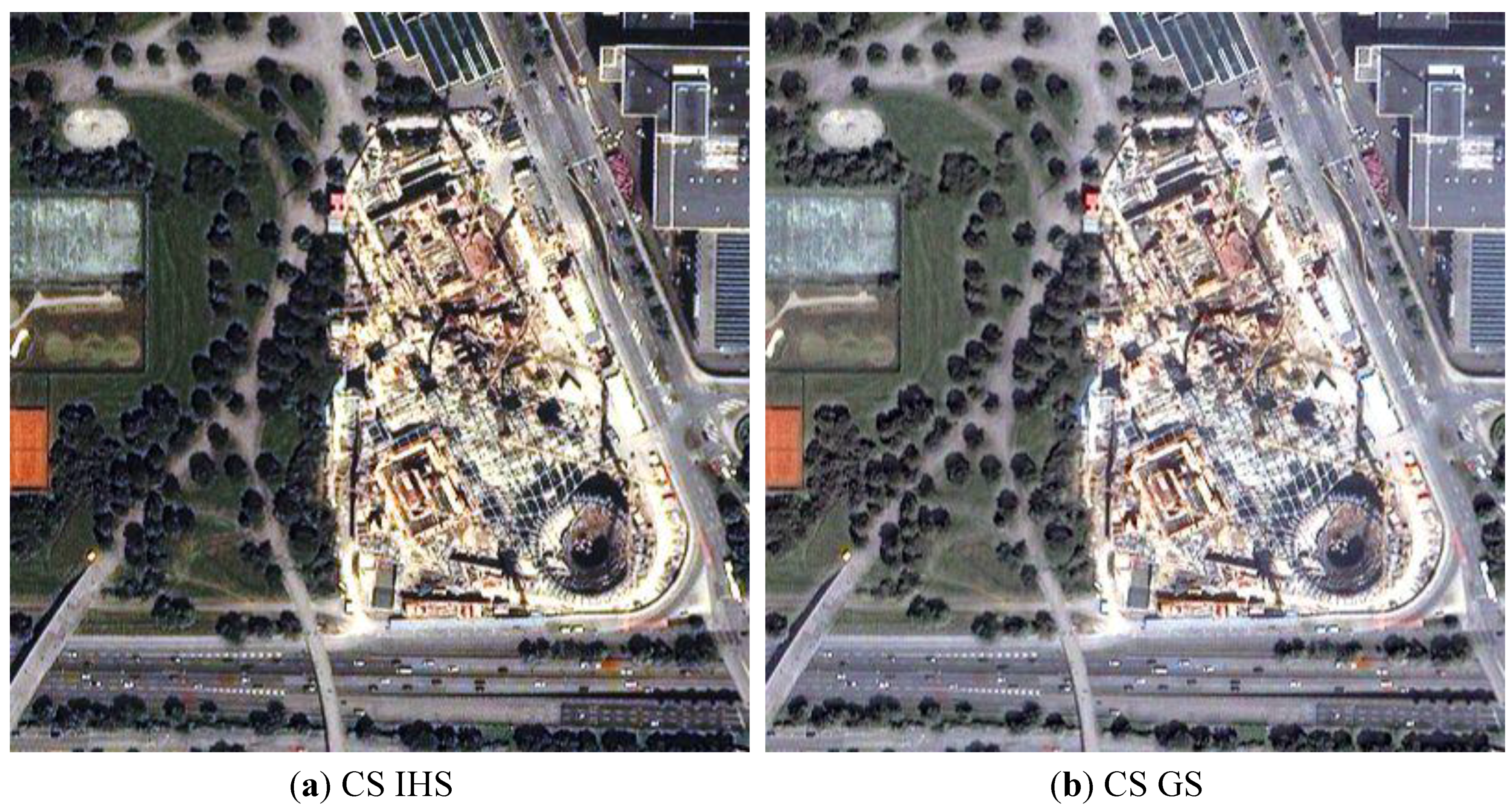
QLR of other methods: CS IHS (method 9 in
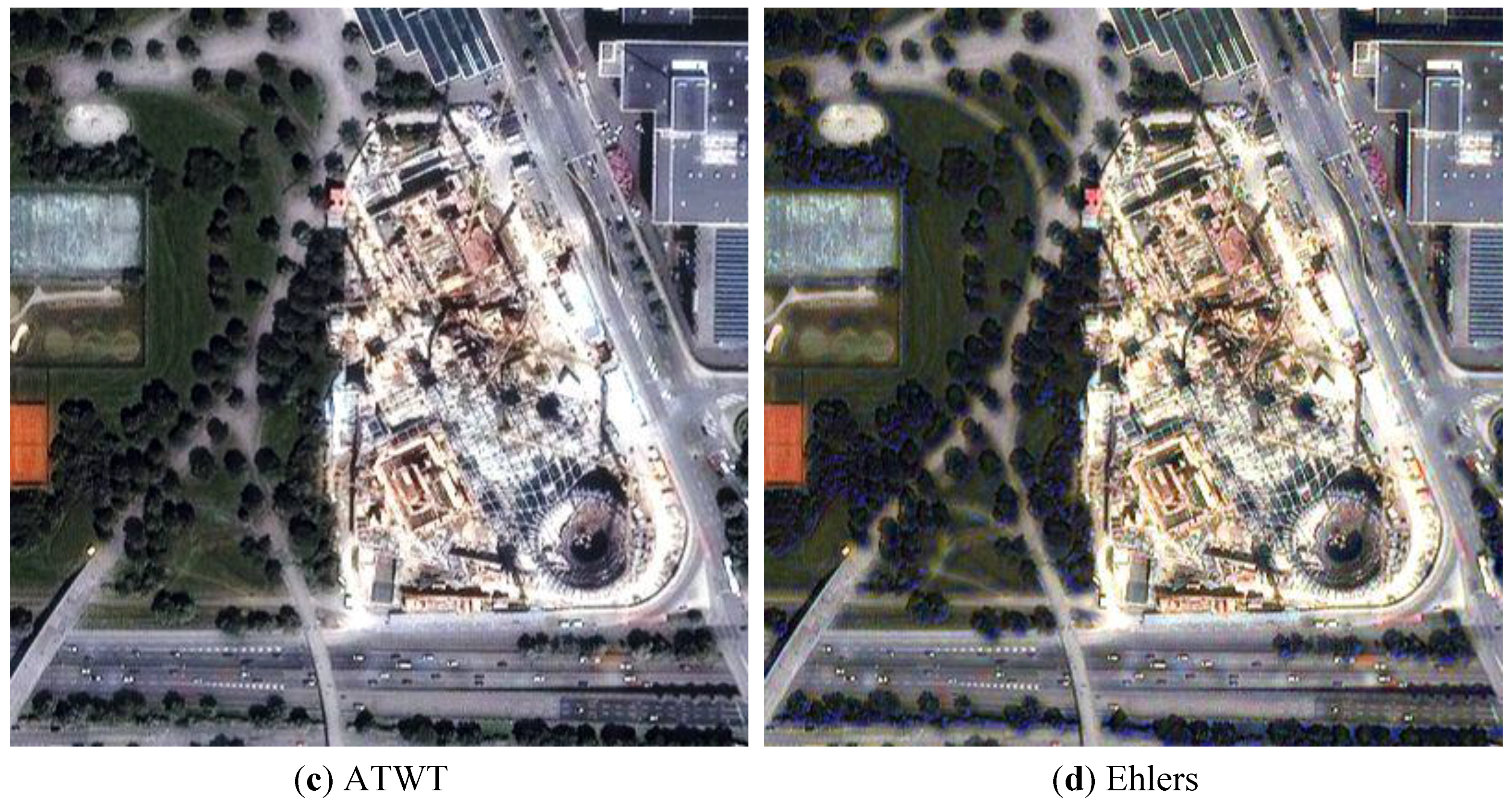
Table 2), CS GS (method 10), ATWT (method 11) and Ehlers (method 12) is lower than those of most filtering methods, whereas for QHR the opposite observation is valid. Finally, JQM of these methods 9–12 is lower than those of the best filtering methods 2–3, 6–7. For example, low JQM of method 10 is well illustrated visually in
Figure 12. The colors of the image in
Figure 12b are significantly different from those of BIL interpolation in
Figure 11a or the best pansharpening method 7 in
Figure 11e. QNR ranks methods 9–12 close to methods 1, 5 with high spatial quality. Only Ehlers (method 12) receives a high overall score.
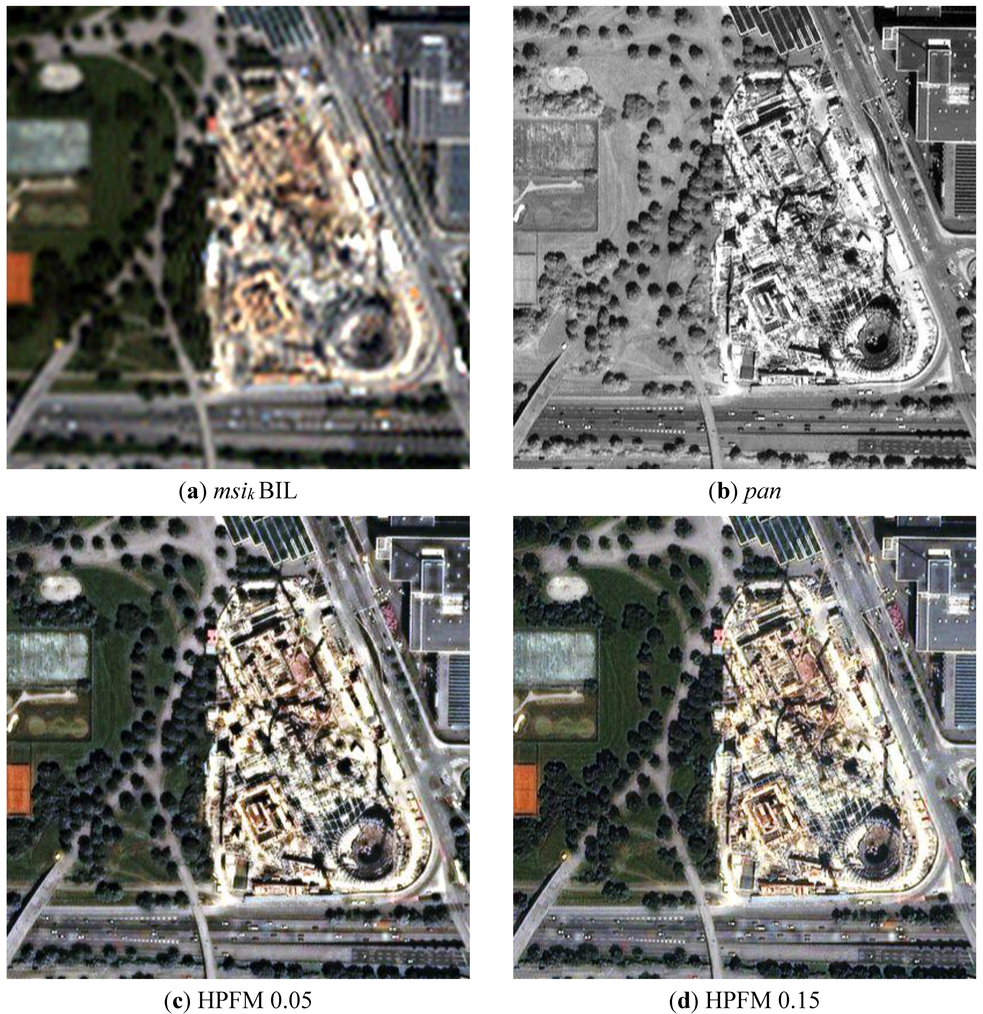
Figure 11.
Bilinear interpolated bands: 3, 2, 1 (a), panchromatic band (b) and HPFM fusion with variable image quality controlled by parameters: 0.05 (c), 0.15 (d), band dependent parameters: 0.3, 0.25, 0.25, 0.1 (e) and 0.7 (f) for IKONOS data.
Figure 11.
Bilinear interpolated bands: 3, 2, 1 (a), panchromatic band (b) and HPFM fusion with variable image quality controlled by parameters: 0.05 (c), 0.15 (d), band dependent parameters: 0.3, 0.25, 0.25, 0.1 (e) and 0.7 (f) for IKONOS data.
Figure 12.
Different fusion methods: CS IHS (a), CS GS (b), ATWT (c) and Ehlers (d) for IKONOS data.
Figure 12.
Different fusion methods: CS IHS (a), CS GS (b), ATWT (c) and Ehlers (d) for IKONOS data.
In conclusion, I mention one more observation or drawback of QNR limiting its practical usage. JQM values of any pansharpening method (
Figure 9a) are higher than those of only interpolation methods (
Figure 1a,
Figure 3a). In contrast, QNR values of all interpolation methods (
Figure 2a,
Figure 4a) are higher than these of all pansharpening methods (
Figure 10a), except methods 4 and 8 whose quality as we know already is estimated wrongly.


