Airborne LiDAR Detects Selectively Logged Tropical Forest Even in an Advanced Stage of Recovery

Abstract

Identifying historical forest disturbances is difficult, especially in selectively logged areas. LiDAR is able to measure fine-scale variations in forest structure over multiple kilometers. We use LiDAR data from ca. 16 km² of forest in Sierra Leone, West Africa, to discriminate areas of old-growth from areas recovering from selective logging for 23 years. We examined canopy height variation and gap size distributions. We found that though recovering blocks of forest differed little in height from old-growth forest (up to 3 m), they had a greater area of canopy gaps (average 10.2% gap fraction in logged areas, compared to 5.6% in unlogged area); and greater numbers of gaps penetrating to the forest floor (162 gaps at 2 m height in logged blocks, and 101 in an unlogged block). Comparison of LiDAR measurements with field data demonstrated that LiDAR delivered accurate results. We found that gap size distributions deviated from power-laws reported previously, with substantially fewer large gaps than predicted by power-law functions. Our analyses demonstrate that LiDAR is a useful tool for distinguishing structural differences between old-growth and old-secondary forests. That makes LiDAR a powerful tool for REDD+ (Reduction of Emissions from Deforestation and Forest Degradation) programs implementation and conservation planning.

1. Introduction

In a world increasingly under anthropogenic pressure, over 300 million hectares of tropical forests have been degraded by anthropogenic activity since 1980 [1,2,3], as reported by the FAO in the report on the state of the world’s forests [4]. However, there are many areas where forests are recovering from anthropogenic disturbance, due to the abandonment of marginal agricultural lands as rural populations migrate into urban areas [5] and because selectively logged forests have little commercial value for many years after timber extraction [6]. One analysis suggests that about 850 million hectares of tropical forest was at some stage of recovery in 2000 [3]. These recovering forests can be of high conservation value [2,7,8,9] and act as globally-important carbon sinks [9,10,11,12]. However, there is much uncertainty regarding the changing extent of regenerating forests, their rate and stage of recovery, and the influence of recovery on further forest exploitation. Here we propose a tool to assist with forest recovery assessments that may be applicable in conservation planning and carbon storage assessments [13,14,15]. Whilst considerable progress has been made in “real-time” detection of logging using satellite multispectral sensors [16,17], selectively logged areas can be very difficult to detect remotely after only a few years of recovery [1,14,18]. Selective logging is the removal of specific trees, of commercial value, and larger than a threshold size [19]. Forest disturbance from selective logging may have enduring effects on forest dynamics and composition [2,12,20,21]. Thus, new approaches are needed to characterize the structure and diversity of forests recovering from human disturbance, given the key role of canopy gaps in forest regeneration processes [22,23] and forest biodiversity through creating habitat heterogeneity for forest dwelling organisms (e.g., [24,25]). Furthermore, the assessment of regeneration dynamics is critical for the definition of sustainable timber extraction schemes; and being able to detect historically disturbed forests could also be particularly important for REDD+ projects, because carbon payments are based on measurable reductions in forest degradation as well as reduced deforestation [26].

Forest canopy gaps are a persistent physical result of disturbance in the forest, thus studying canopy gaps may shed light on logging history, even where there is a lack of accurate data regarding the extent of disturbance. There has been recent interest in the analysis of canopy gaps using airborne Light Detection and Ranging (LIDAR) data. This technology produces detailed 3-D point clouds of leaf and stem locations within forests, from which canopy surface and terrain models can be produced and then sliced into horizontal planes to produce high-resolution maps of gap locations across a range of height tiers [27,28,29,30,31]. This extends the traditional definition of a gap from the canopy down to ground level [32]. Ground-based LiDAR was successfully used to measure canopy structure in different types of forests (e.g., [33,34]). A recent study [35] compared structural canopy metrics measured using both airborne and terrestrial LiDAR scans. They concluded that, while the airborne LiDAR had restricted ability to estimate stem volume, both techniques gave similar estimates of canopy height and vertical distribution of foliage and leaf area. In contrast to discrete return LiDAR, which is not suitable to estimate stem structure, full waveform, both airborne [36,37,38] and satellite-based LiDAR [39,40,41] was used successfully recently to estimate canopy structural characteristics, such as timber volume and basal area.

Before the development of these LiDAR-based techniques, few studies had characterized gap frequency distributions because of the laborious nature of field-based methods [42]. However, using LiDAR data, it was possible to locate the position of nearly six million gaps >1 m² in an area of 125,581 ha of lowland Amazonian forest in Peru [28]. Studies of gap size distributions using LiDAR have generally found that these distributions followed a power-law, with a scaling exponent that varied with disturbance regime (e.g., [27,28,29]). If selectively logged forests have distinctive gap characteristics that are preserved, to some extent, late into the recovery process, then the finely resolved structural data from LiDAR may be successful in identifying past disturbance where other methods have failed.

Here we use airborne LiDAR imagery to explore whether selectively logged forests in West Africa that have been recovering for at least 23 years, could be distinguished from old-growth forests in terms of gap size distributions and height characteristics. We compare four contiguous patches of moist tropical forest, three of which were selectively logged in 1960–1989, and one of which is old growth. Although few records have been kept (which is typically the case in developing countries; [43]), we know that logging concessions granted the removal of large timber trees (>50 cm stem diameter) whilst retaining smaller trees and less-favored species. We hypothesized that: (1) the top height of logged forest would be lower than that of old-growth forest, even after 23 years of recovery [12]; (2) the total area of gaps (hereafter “gap fraction”) within a given height tier of the canopy would be greater in recovering forest; (3) gap sizes would be power-law distributed and the power-law exponent will be most negative in old-growth forest, because large gaps are less common in this forest type; and (4) some ground-level canopy gaps created by selective logging would endure for many years resulting in an altered gap size distribution. We then use our conclusions from these analyses to propose a novel way to map the forest according to disturbance history. We ground-truth our remote sensing results using data collected from an extensive network of permanent inventory plots [44].

2. Experimental Section

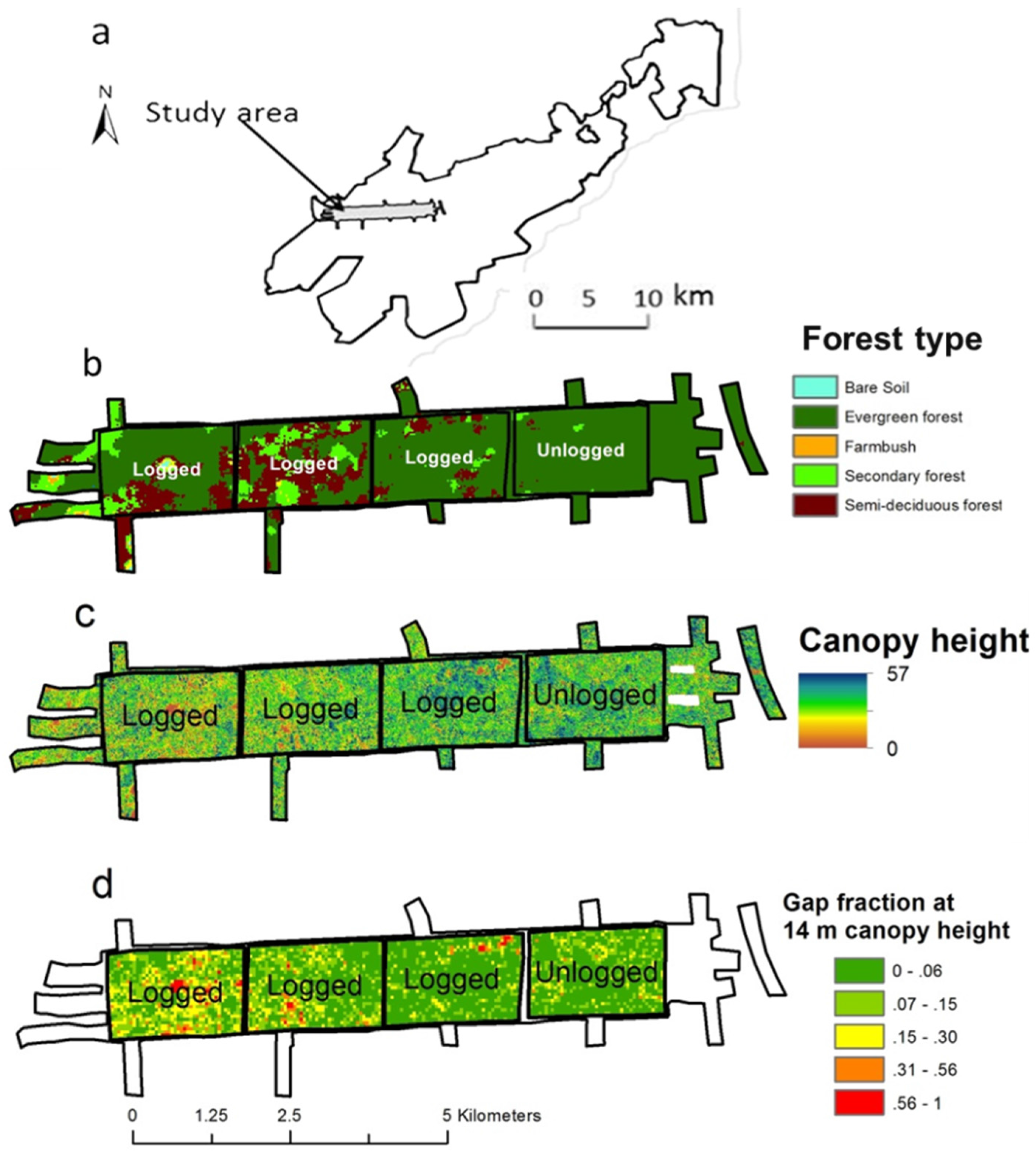
2.1. Study Area

Gola Rainforest National Park is located along the border between Sierra Leone and Liberia, West Africa, between 7°18ʹ and 7°51ʹN and 10°37ʹand 11°21ʹW (Figure 1). It is one of the largest tracts of intact lowland forest in West Africa. The forest accommodates over 300 tree species and is the habitat of a large number of animals threatened by regional forest loss and degradation [44,45]. Annual precipitation is 2500–3000 mm, mostly falling in a wet season between May and October. Around 30% of Gola forest was selectively logged between 1960 and 1989 (logging mostly consisted of trees >50 cm DBH), but most detailed records have been lost [44]. Our study concentrated on a stretch of forest of ~16 km² in the central region of the park. Within the study area, we manually delineated four 3 km² blocks within the extent of the LiDAR swath for analysis (Figure 1). The three western blocks were selectively logged (9 km²), and timber was processed at a sawmill located just outside the northwest corner of the study area. The most easterly of these three blocks (hereafter Block 2), which was furthest from the mill, was less heavily logged (according to a former employee of a logging company interviewed by D.A. Coomes and J. Lindsell). The central (hereafter Block 3) and the western block (hereafter Block 4) were closest to the sawmill, and presumably suffered the heaviest logging, The eastern block (hereafter Block 1) was considered old-growth forest (3 km²). Commercial logging has now ceased, although there has been some small-scale felling near villages to the west.

Figure 1. (a) A map showing the boundaries of Gola National Park (black) and the study area (grey); (b) division of the study area into equal-area blocks for the gap size frequency analyses, with forest types shown (see [46] for details); (c) a canopy height model derived from LiDAR cloud point; and (d) estimated gap fractions within the 14–15 m height tier, estimated from the LiDAR point cloud, in 0.25 ha sub-blocks. The blocks were numbered, from east to west: 1, unlogged block; 2, eastern logged block; 3, central logged block; and 4, western logged block.

Figure 1. (a) A map showing the boundaries of Gola National Park (black) and the study area (grey); (b) division of the study area into equal-area blocks for the gap size frequency analyses, with forest types shown (see [46] for details); (c) a canopy height model derived from LiDAR cloud point; and (d) estimated gap fractions within the 14–15 m height tier, estimated from the LiDAR point cloud, in 0.25 ha sub-blocks. The blocks were numbered, from east to west: 1, unlogged block; 2, eastern logged block; 3, central logged block; and 4, western logged block.

It should be noted that since our dataset consisted of a single LiDAR swath over a continuous stretch of forest, with logged forests at one end and intact forest at the other, it is possible that canopy changes we observe along the east–west gradient are not entirely attributable to logging [47]. We found that aspect, slope and rainfall did not vary across the swath and thus we did not account for them in further analyses; although we lack detailed soil type information, it is not thought to vary systematically across the survey areas. However, we cannot completely rule out the possibility of an unobserved covariate. The generality of our study will only become apparent with time, when summary statistics from future LiDAR surveys are compared with ours, perhaps using a meta-analysis approach. For the moment, test statistics reported here need to be treated with caution, because within “treatment” replication is used in comparisons [47].

2.2. LiDAR Data

LiDAR data of the study area were collected during 20–22 March 2012, using discrete returns from an Optech ALTM Gemini device, with high pulse densities used to penetrate the dense forest canopy (>10 pulses per m²). Data were processed using TIFFS software [48] to produce a canopy height model (CHM) and, from the ground returns, a digital elevation model (DEM), both at 1 m spatial resolution. The elevation, aspect and slope of each 1 m pixel was extracted from the DEM using ArcGIS [49].

2.2.1. Canopy Surface Height

We analyzed factors affecting canopy surface height, the most obvious measure of forest recovery from disturbance, using multiple linear regression. We selected 1000 random locations throughout the study area and calculated the mean canopy height of a 10 × 10 m pixel “neighborhood” centered on the sampling location. Mean elevation, aspect, slope and topographic position index [50] were calculated for each neighborhood, and used as explanatory variables alongside a binary variable indicating whether the location was within one of the blocks subjected to logging. We used least-squares regression in R version 2.15.2 [51] to estimate the effect of explanatory variables on canopy height, using F-tests to select a minimum adequate model. To compare between canopy surface heights in the different blocks, we calculated the mean and standard deviation of the CHM within each block.

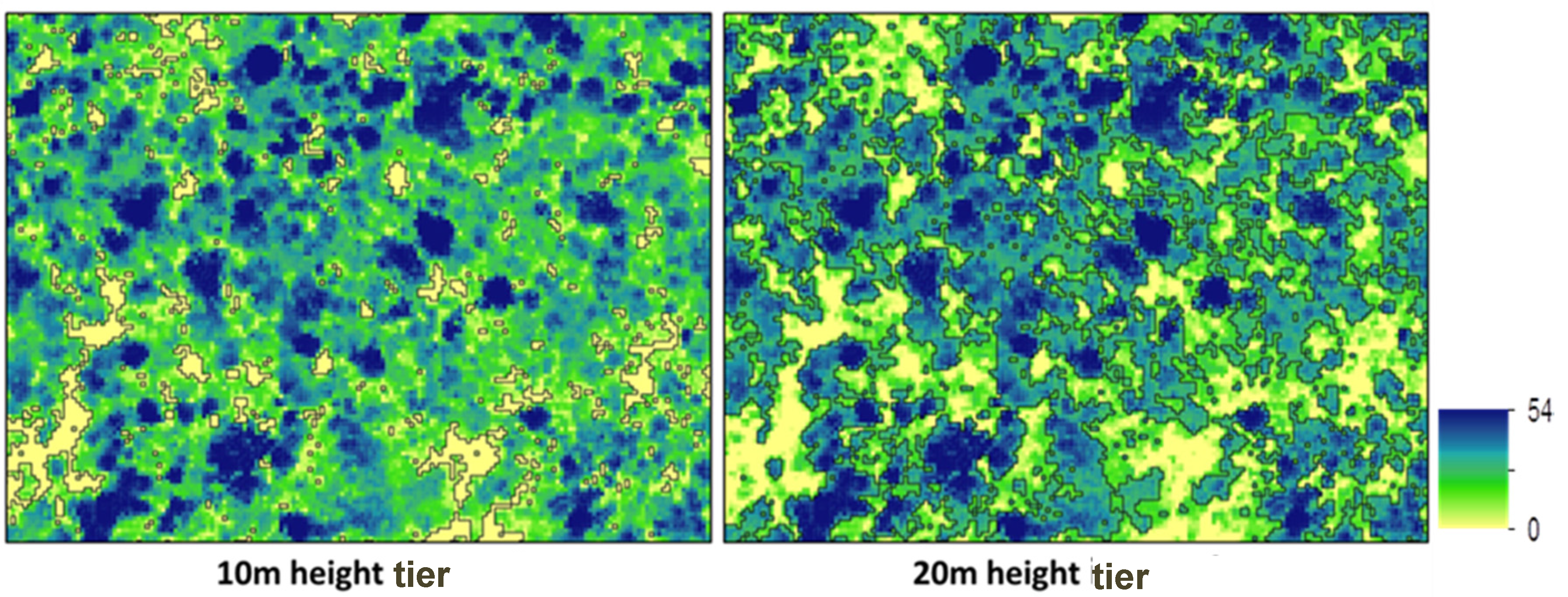
2.2.2. Gap Size Distribution

For the gap-size distribution analyses, we resampled the CHM at a horizontal resolution of 3 × 3 m, and made 9 m² the minimum gap size we detected. We chose not to work with 1 m² gaps (cf. [27,28]) because laser pulses are angled at up to 20° from the nadir by the LiDAR device, and this can result in biases when detecting small gaps [52]. We analyzed the distribution of canopy gap sizes in each 1 m height tier in the logged and old growth sections of the study area, following the methodology of [27]. We divided the canopy height data into 1 m height tiers, between 2 and 22 m. At each height tier, discrete groups of unoccupied pixels surrounded by filled pixels were defined as canopy gaps; these gaps were recognized as polygons by ArcGIS version 10 (Figure 2), and the same software was used to measure the sizes of all gaps found in each height tier [49]. The reason for analyzing gaps only to 22 m height is that gaps start to coalesce above this height, with a marked decrease in gap frequency.

Figure 2. A section of the forest in Gola, represented by LiDAR-derived CHM, showing gaps (delineated by dark line) at the 10 m height tier (left) and 20 m height tier (right), in the same location. Cold colors represent taller canopy and warm colors represent shorter canopy.

Figure 2. A section of the forest in Gola, represented by LiDAR-derived CHM, showing gaps (delineated by dark line) at the 10 m height tier (left) and 20 m height tier (right), in the same location. Cold colors represent taller canopy and warm colors represent shorter canopy.

Recent studies have fitted a discrete power-law distribution (known as a zeta distribution) to gap-size frequency distributions [27,28]. The probability distribution function (PDF) of a zeta distribution is:

$$f\left(A\right)=\frac{A^{-\text{λ}}}{\text{Ϛ}\left(\text{λ}\right)}$$

(1)

where A is gap size (an integer, m²), $-\text{λ}$ is the scaling exponent ($\text{λ}>0)$, and $\text{Ϛ}\left(\text{λ}\right)$ is a normalization function, ensuring the probability density function sums to 1 over all values of A. The expected number of gaps of size A is given by $n\left(\text{A}\right)=N{A}^{-\lambda }/\text{Ϛ}\left(\lambda \right)$, where N is the total number of gaps. The log–log transformation gives the familiar power-law function:

$$\log \left(n\left(A\right)\right)=\text{ α}-\text{λ}\log \left(A\right)$$

(2)

where $\text{α}=\text{log}\left(N/\text{Ϛ}\left(\text{λ}\right)\right)$. None of the recent LiDAR studies has checked whether a power law was the statistically best-supported function to describe the frequency distribution. A simple test is to plot $\log \left(n\left(A\right)\right)$ against $\log \left(A\right)$ and observe whether the data fall along a straight line. Our examination of the plots presented in [27,28,29] suggested downward curvature in some instances, so we tested for deviations from a power-law distribution by introducing a quadratic term:

$$\log \left(n\left(A\right)\right)= \alpha -\text{λ}\log \left(A\right)-\text{β}{\left(\log \left(A\right)\right)}^2$$

(3)

where β is a quadratic modifier (β >0; cf. [53], and n(A) is the expected number of gaps of size A. The probability density function for this modified power function is:

$$\text{p}{\left(A\right)}_z= \text{τ}{A}^{-\left(\text{λ}+\text{β}\log \left(A\right)\right)}$$

(4)

where $\text{τ}$ is a normalizing constant that ensures that the probability of all possible outcomes is 1 when summed over all gap areas sampled, even if the data are truncated (i.e., minimum area > 1). The z subscript indicates this is the PDF for height tier z above the forest floor.

We used a Bayesian Markov Chain Monte Carlo estimation to estimate the values of λ and β for the four blocks, using the FilzbachR package [54]. At each iteration of the search algorithm, we calculated the sum of $A^{-\left(\text{λ}+\text{β}\log \left(A\right)\right)}$ across all possible values of A, in order to calculate τ. We used uninformative priors, a burn-in phase of 20,000 iterations and a sampling phase of 50,000 iterations; we sampled every 50th iteration to generate the posterior distribution. In order to test for the convergence of parameter values, we plotted three chains sampling the posterior distribution.

To test whether the modified power function had stronger statistical support than the power function, we compared the alternative models using BIC (Bayesian Information Criterion; [55]. We also tested whether logged vs. old-growth forests had different size-frequency distributions by fitting a single model to all four blocks and comparing that with models fitted to the blocks individually. Using the predictions of the separate block model, we estimated gap fractions per height tier in the different blocks.

2.3. Canopy Height and Gap Fraction Estimates from Ground Sampling Plots

We compared our LiDAR-derived statistics with gap fractions and height metrics estimated from permanently marked inventory plots from across the Gola reserve in order to both validate our LiDAR analyses and compare them to a wider area of continuous forest. The ground data were collected from a gridded network of 697 permanent plots, each of 0.125 ha, established within Gola Rainforest National Park in 2005–2007 to provide unbiased estimates of carbon stocks (see [31] for details). Each plot was geo-located using a hand-held Garmin GPS device. To increase accuracy, the device was allowed to re-sample the location for as long as the team stayed in the plot and the location was determined using the average reading from each plot. Prior to our study, 266 of the inventory plots had been classified as old-growth, 119 as having undergone well-managed logging and 166 as having undergone poorly-managed logging. The rest of the plots were classified as disturbed and were not included in the analyses, as the LiDAR data did not include areas that fitted that disturbance category. Classifications were based on expert knowledge of the logging history [44]. Stem diameters at breast height (DBH), or immediately above buttresses, of all trees >30 cm DBH were measured in these plots. In addition, the diameters of trees >10 cm DBH were measured within 0.0125 ha subplots. The dataset consisted of 8771 trees (307 species) of which 6471 trees (253 species) were found in the 0.125 ha plots, and 2300 trees (232 species) in the 0.0125 ha sub-plots. Frazer et al. [56] showed that plots of that size (0.125 ha) provide reasonable ground truth data for LiDAR studies. Of those 697 plots, 20 were located inside our study area.

The mean canopy top height of each plot was estimated from the height and crown dimension of constituent trees. First, we fitted allometric relationships to 348 measurements of DBH, height and crown diameters from 56 species collected in Gola [57]. We fitted allometric (i.e., log–log) relationships between height and DBH and between crown diameter and DBH in FilzbachR, using hierarchical modeling to allow species to have different intercepts drawn from a normal distribution whilst keeping the allometric slope constant among species. Secondly, we used these allometric relationships to predict the crown diameter and height of all recorded trees in the 697 plots (8770 trees); species-specific allometries were used to make these predictions for 56 species (16% of trees) while mean allometric coefficients were used for the remaining species. We then assumed that crowns were truncated spheroids (which [58] argue is realistic for temperate angiosperm trees) and by integration determined the vertical distance from the tree top at which cumulative crown area was half the total crown area, which we assumed to be the “effective” height of trees, as viewed by LiDAR; we lacked information about the precise spheroid form of Gola trees, so used information from studies published elsewhere (see [58,59] and Supplementary Information), from which we calculated that (effective height) = 0.84 × (tree height). Finally, the effective height of each tree was weighted by its proportional contribution to total crown area to calculate the mean canopy top height. This refinement of the mean Lorey’s height (height weighted by tree basal area) gave height estimates for all field plots (n = 697) including those within the LiDAR survey (n = 20). We also estimated the vertical profile of canopy gap fraction from field-plot data, and used these profiles to compare the effects of different management regimes. For each of the permanent field plots, we estimated crown areas and heights of all recorded trees from their stem diameters (DBH > 10 cm), as described above. For a given height tier (>11 m height), we then summed the crown areas of all trees taller than that height, and divided by ground plot size to get cumulative crown area per unit ground area (CCA). Using results from the old-growth plots, we related the mean CCA in each height tier to the mean gap fraction estimated by LiDAR for the same height tier, using least squares regression. This gave us an equation for converting CCA values to gap fractions. We applied this equation to estimate gap fractions in well- and poorly-managed logged forests across the permanent plots. Note that the old-growth gap-fraction curve obtained from plot data is practically identical to that obtained from LiDAR data because the latter data were used to generate it. The approach is useful, nevertheless, for comparing the effects of management on gap fraction. Overall, we measured and assessed several canopy structural features using both field data and LiDAR derived data, including canopy surface height, gap fraction (the percent of the area in the canopy consisting of gaps), and gap size distributions. See Table 1 for a comprehensive list of variables [34,44,57].

Table 1. A list of canopy structure variables used in the study, including field- and LiDAR-based estimates of canopy height and gap fraction.

Variable	Data Source	Variable Description
LiDAR Canopy surface height	LiDAR	The mean height of the canopy as extracted from the first returns of the LiDAR point cloud over the entire 3 km2 blocks, at 1 m2 resolution
Field Canopy surface height	Field plots [44]	The heights and crown areas of all tagged trees within a plot were estimated from diameters using site- and species-specific allometries [57]. The height of each tree was weighted by its proportional contribution to the total crown area when calculating mean canopy surface height
LiDAR Gap fraction	LiDAR	Total area of gaps per height tier in the canopy height model, divided by block area (3 km2)
Field Gap fraction	Field plots [34]	Evaluation of gap fraction in the field plots, by summing crown areas of all trees in the plot, and subtracting it from plot size
Gap size distribution parameters	LiDAR	The scaling exponent (λ) and quadratic modifier (β) of the gap size frequency distribution, estimated using an MCMC sampling procedure

Table 1. A list of canopy structure variables used in the study, including field- and LiDAR-based estimates of canopy height and gap fraction.

Variable	Data Source	Variable Description
LiDAR Canopy surface height	LiDAR	The mean height of the canopy as extracted from the first returns of the LiDAR point cloud over the entire 3 km2 blocks, at 1 m2 resolution
Field Canopy surface height	Field plots [44]	The heights and crown areas of all tagged trees within a plot were estimated from diameters using site- and species-specific allometries [57]. The height of each tree was weighted by its proportional contribution to the total crown area when calculating mean canopy surface height
LiDAR Gap fraction	LiDAR	Total area of gaps per height tier in the canopy height model, divided by block area (3 km2)
Field Gap fraction	Field plots [34]	Evaluation of gap fraction in the field plots, by summing crown areas of all trees in the plot, and subtracting it from plot size
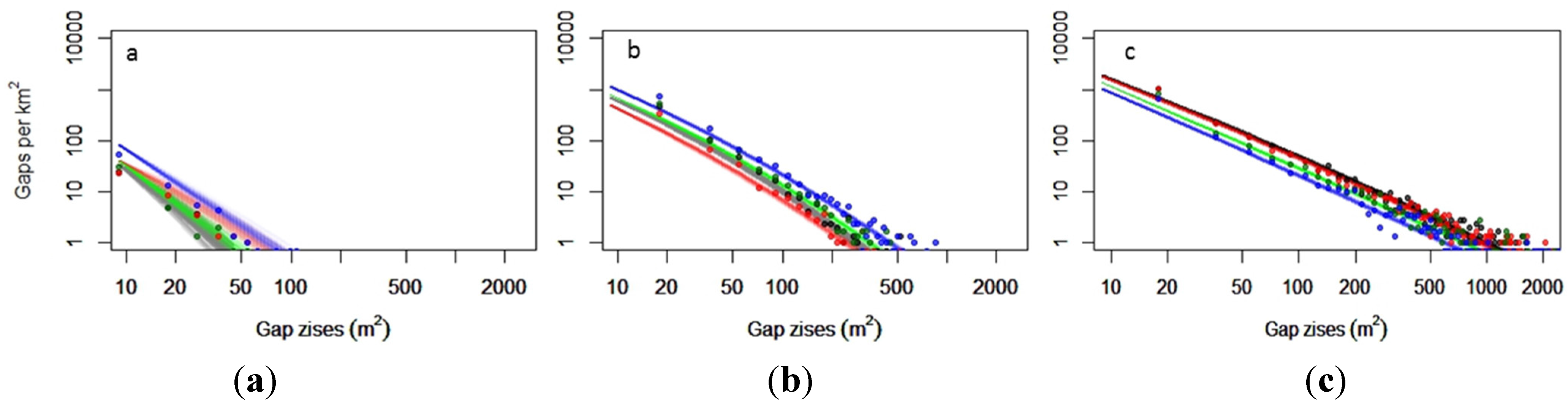
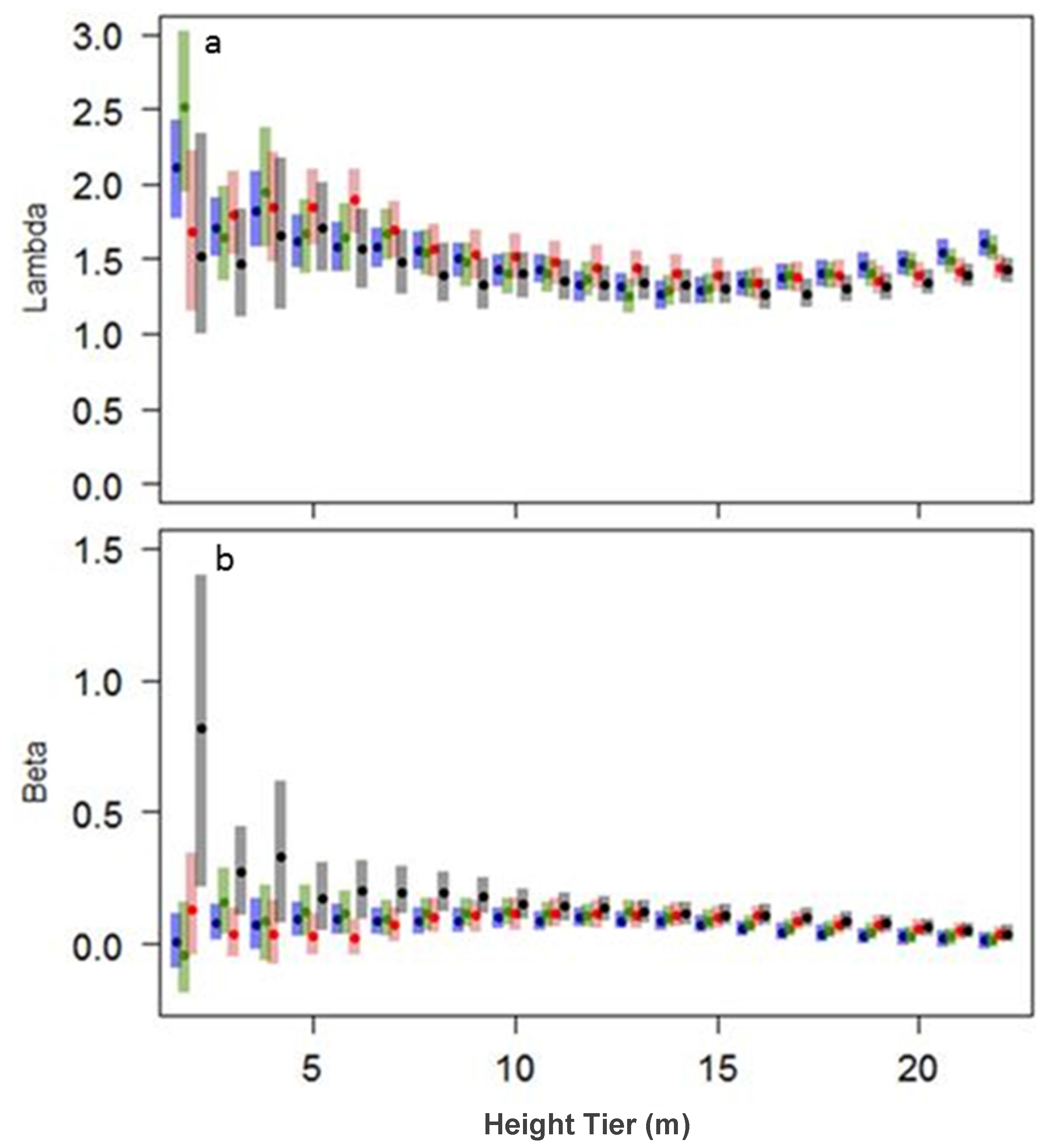
Gap size distribution parameters	LiDAR	The scaling exponent (λ) and quadratic modifier (β) of the gap size frequency distribution, estimated using an MCMC sampling procedure

3. Results and Discussion

3.1. Results

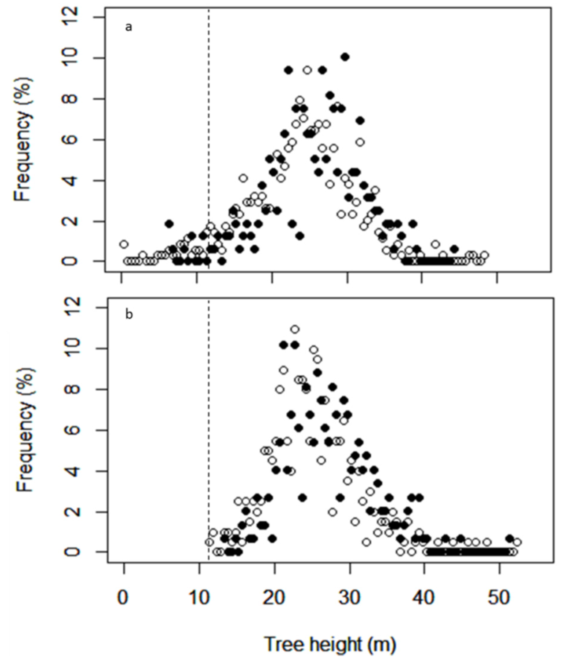
3.1.1. Canopy Height

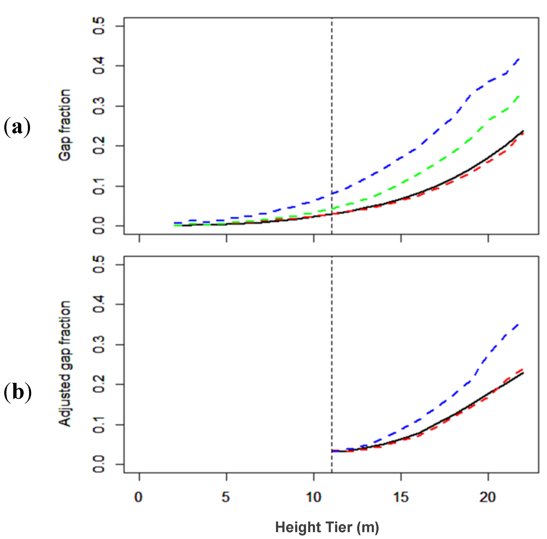
We found a significant difference in mean canopy height between recovering and old-growth forest. The emerging linear model was

$$\text{Canopy height}=24.43-0.88\times \text{elevation}-0.69\times \text{logging status}$$

(5)

where logging status is a binary variable indicating whether the sampled location was logged or not, and elevation is scaled (i.e., mean of zero and standard deviation of one), to allow direct effect-size comparisons. However, although there was a statistically significant difference in height (Figure 3) at 1000 sampled locations (F_{1, 994} = 10.4, p = 0.001) the model had low explanatory power (R² = 0.03) and the effect size was small and only apparent in the western blocks in which logging had been heaviest. Mean heights (± standard deviation) were 22 ± 6.7 m, 23.6 ± 6.2 m and 25.8 ± 5.9 m in Blocks 4, 3, and 2, respectively (west–east logged blocks), compared with 25.6 ± 5.7 m in the old-growth Block 1. Permanent plot data showed a similar pattern with mean crown-area-weighted heights slightly lower in disturbed and over-logged plots (20.5 ± 5.8 m and 20.6 ± 5.8 m, respectively, after correcting for crown shape by multiplying by 0.84) than in well-managed and undisturbed plots (22.0 ± 5.8 m and 22.7 ± 5.8 m, respectively, after shape correction). Mean canopy surface height was negatively affected by elevation (F₁₉₉₄ = 20.8, p = 0.0001) and this effect was more pronounced than logging history according to a linear regression model. Within old-growth locations predicted mean canopy surface height decreased from 26.5 m to 21.5 m between 300 m and 460 m elevation (the minimum and maximum elevations observed). Logging history and elevation were the only explanatory variables that significantly influenced canopy height in a multiple regression analyses (at p < 0.05).

Figure 3. (a) Distribution of canopy height frequencies in the recovering logged (open symbols) and old-growth (solid symbols) blocks in the study area. The mean heights were 23.9 and 25.6 m, while standard deviations were 6.4 and 6.9, respectively. Panel (b) is the mean weighted height frequency of trees in the permanent field plots. Minimum height (11 m), noted by the vertical dashed lines, was dictated by the minimum size of trees measured in the plots [44]. Mean weighted height in plots classified as unlogged was 22.7 ± 5.8 m, while mean weighted height was 20.5 ± 5.8 m in the plots classified as disturbed.

Figure 3. (a) Distribution of canopy height frequencies in the recovering logged (open symbols) and old-growth (solid symbols) blocks in the study area. The mean heights were 23.9 and 25.6 m, while standard deviations were 6.4 and 6.9, respectively. Panel (b) is the mean weighted height frequency of trees in the permanent field plots. Minimum height (11 m), noted by the vertical dashed lines, was dictated by the minimum size of trees measured in the plots [44]. Mean weighted height in plots classified as unlogged was 22.7 ± 5.8 m, while mean weighted height was 20.5 ± 5.8 m in the plots classified as disturbed.

3.1.2. Gap Fraction

In support of our second hypothesis, gap fraction in Block 4 (western) (6.3% at 10 m) and Block 3 (central) (3.4% at 10 m height) logged blocks was higher than in the old-growth Block 1 (2.3% at 10 m height). In Block 2, which was least affected by logging, the gap fraction was similar to that in the old growth block (2.3% at 10m height tier, Figure 4a). To compare gap fractions estimated from field and LiDAR data, we fitted a least squares regression to the gap fractions, as a function of height above the ground (see Methods section for details). The fitted line followed the function:

$$\text{Gap fraction}=1-\left(-0.44+2.5\times {\text{height}}_{\text{i}}-1.11\times {{\text{height}}_{\text{i}}}^2\right)$$

(6)

Gap fractions estimated using LiDAR were similar to those estimated from field plots, ranging between c 0.5% at 2 m height, and c 25% at 22 m height in the unlogged and well-managed logged plots, and between c 0.5% at 2m height and c 35% at 22 m height in the heavily logged plots ([31], Figure 4b).

Figure 4. Gap fractions at different height above the forest floor, estimated from (a) airborne LiDAR and (b) permanently marked field plots. In the upper panel, curves from old-growth forest (solid black line), heavily logged forest (dashed blue and green lines) and less heavily logged forest (dashed red line) are shown (corresponding to blocks shown in Figure 5). In the lower panel, curves from unlogged sites (solid black line), well-managed logged sites (red) and poorly-managed logged sites (blue) are compared (minimum height = 11 m because only trees >10 cm DBH were recorded in the plots). We adjusted the estimates of gap fraction to account for overlap between individual tree crowns, by fitting them with the curve parameters extracted from LiDAR derived gap fractions. Gap fraction estimates indicate that the well-managed logged areas recovered back to their state prior to logging in terms of gap fraction.

Figure 4. Gap fractions at different height above the forest floor, estimated from (a) airborne LiDAR and (b) permanently marked field plots. In the upper panel, curves from old-growth forest (solid black line), heavily logged forest (dashed blue and green lines) and less heavily logged forest (dashed red line) are shown (corresponding to blocks shown in Figure 5). In the lower panel, curves from unlogged sites (solid black line), well-managed logged sites (red) and poorly-managed logged sites (blue) are compared (minimum height = 11 m because only trees >10 cm DBH were recorded in the plots). We adjusted the estimates of gap fraction to account for overlap between individual tree crowns, by fitting them with the curve parameters extracted from LiDAR derived gap fractions. Gap fraction estimates indicate that the well-managed logged areas recovered back to their state prior to logging in terms of gap fraction.

3.1.3. Gap-Size Distributions

The hypothesis that gap sizes are power-law distributed was rejected. A modified power-function was much more strongly supported at most height tiers, except 2 and 4 m above the ground, where the power-law model was slightly superior (change in Bayesian Information Criterion (BIC) of 1.4 and 0.6, respectively; Figure 5). The models using the modified power law performed better in terms of the BIC, with the change ranging between 0.6 and −678. Changes in BIC greater than 10 are considered substantial [60]. The deviations from a power law had a large impact. At the 10 m height tier in the old-growth block, the simple power-law predicted 27 gaps/km² (gaps ≥ 100 m²), while the modified power-law model predicted no gaps at all above this size threshold. Generally, deviations from a simple power-law were greater in the lower height tier (the modifier parameter β had relatively more negative values), indicating that large gaps were less frequent in the lower height tiers than expected by a simple power-law (Figure 6).

Figure 5. Predicted (lines) and observed (points) frequencies of canopy gap sizes per km², in the four blocks in Gola, at 2 m (a), 10 m (b) and 22 m (c) canopy height tiers. Grey represents block 1; green is block 2; red is block 3; and blue is block 4. Lines are based on the modified power-law distribution function with quadratic term. Lines represent predictions using 100 values selected randomly from the posterior distribution of model parameters.

Figure 5. Predicted (lines) and observed (points) frequencies of canopy gap sizes per km², in the four blocks in Gola, at 2 m (a), 10 m (b) and 22 m (c) canopy height tiers. Grey represents block 1; green is block 2; red is block 3; and blue is block 4. Lines are based on the modified power-law distribution function with quadratic term. Lines represent predictions using 100 values selected randomly from the posterior distribution of model parameters.

The fourth hypothesis that old-growth forest would have a different gap size distribution compared to logged forest was supported by the scaling parameter (λ) values being generally higher for logged (1.26–2.51) than unlogged forest (1.26–1.65), particularly in the lower height tiers of the canopy (Figure 6a). Model selection statistics showed differences in BIC ranging between 4.5 (the traditional power-law model is slightly superior) and −18.4 (the modified model is substantially better), according to the height tier. The scaling and modifier parameters (λ and β, respectively) of the modified power-law model, using a separate model per block, varied among height tiers and gap sizes (Figure 6). The log–log transformed plots of the gap size frequency distributions predicted by the modified power-law model revealed that the differences between the recovering logged and old-growth blocks were greatest in the lower height tiers, and decreased with increasing height above the ground, in support of hypothesis four. At 10 m height, the predicted frequency distribution function of the old growth block converged with the predicted frequency distribution function of the eastern logged Block 2. At 22 m height above the ground all blocks had similar gap size frequency distributions (Figure 5 and Figure S1).

Figure 6. Values of λ (top panel) and β (bottom panel) estimated by fitting a modified power law function to the frequency distribution of canopy gap sizes observed at various heights above the forest floor, in four forest blocks in Gola National Park, Sierra Leone. Points are mean λ and β values estimated for a range of height tiers within the canopy; bars denote 95 % credible tiers. Color scheme follows Figure 5.

Figure 6. Values of λ (top panel) and β (bottom panel) estimated by fitting a modified power law function to the frequency distribution of canopy gap sizes observed at various heights above the forest floor, in four forest blocks in Gola National Park, Sierra Leone. Points are mean λ and β values estimated for a range of height tiers within the canopy; bars denote 95 % credible tiers. Color scheme follows Figure 5.

3.1.4. Mapping Areas of Forest Recovering from Disturbance

The foregoing analyses were used to select the 14 m height tier as an intermediate canopy height for which differences in gap fraction were relatively large. We calculated the gap fraction at this height tier for each 0.25 ha sub block within the study site, and classified the results into 5 levels, using natural breaks. The resulting map (Figure 1d) revealed that the number of these sub-blocks that had at least 30 % gap area at 14 m height (i.e., the two highest gap fraction categories) increased from nine in the unlogged block to 27 in the eastern logged block. In the central and western logged blocks, such sub-blocks covered substantial parts of the area of the block, emphasizing the value in using this gap fraction to identify an historic logging intensity gradient.

3.2. Discussion

3.2.1. Canopy Height

Structural recovery of forests from disturbance depends on the severity of disturbance and the time since it occurred, but rates vary considerably with forest type and environmental factors [61,62]. The mean canopy surface height of selectively logged forest in our West African study was only slightly lower than that of old-growth forest after a quarter century since the termination of logging, and virtually indistinguishable in the less-heavily logged block (Figure 3a). These findings were strongly corroborated by field measurements taken in 697 permanent forest plots in Gola (Figure 3b), distributed over a larger area than the LiDAR survey, and over a wider range of disturbance intensities, ranging from old-growth forest to very disturbed plots. This accords with results from elsewhere. After just five years of recovery, Villela et al. [63] reported that canopy height was the main difference in canopy structure between disturbed and undisturbed stands in an Atlantic forest in Brazil. Okuda et al. [64] also found that the canopy of a dipterocarp forest recovering from selective logging in Malaysia had a distinct height distribution compared with old-growth forest after 23 years of recovery, although mean heights differed by only 2.6 m in that case. Fifty-five years after logging, Brearley et al. [65] reported complete recovery of canopy structure in a secondary mixed lowland forest consisting of tropical rain forest and heath forest in Central Kalimantan, Indonesia. A meta-analysis of structural forest recovery studies [12] found that different structural components of forests recover at different rates. Above ground biomass took about 85 years on average. In terms of canopy height, the part of Gola forest we studied had nearly completely recovered from selective logging after 25 years. Although we have not investigated how rapidly different elements of forest biodiversity and ecosystem functioning recovers from selective logging, a recent review suggests that carbon stocks are much faster to recover than biodiversity [12].

3.2.2. Gap Fractions

Gap fraction estimated from LiDAR was greater in selectively logged than old-growth forest, in concordance with [66]. Higher gap fractions in the lower canopy of recovering forests suggest that the persistence of gaps reaching the forest floor may have been caused by removal of the “advanced regeneration” (i.e., juveniles of canopy species that grow for many decades in the forest understory) during selective logging [67], to facilitate the extraction of timber. In support of that, we found significant differences in dbh of trees in logged and unlogged permanent field plots (one-way ANOVA, F_3,8767 = 15.6, p < 0.001); this is a conservative estimate, as the smallest trees in the samples had stem diameters of 10 cm. As regeneration in canopy gaps is often dominated by established saplings of shade-tolerant species, taking advantage of improved light and nutrient availability [22,67], naturally occurring gaps have a different recovery process than logging-related gaps, in which many of these saplings are removed [67,68]. Furthermore, damage to the soil during timber removal has been shown to affect regeneration processes in canopy gaps [14,16]. Our results show that these sorts of impacts from selective logging can be detected many years after logging as ceased.

3.2.3. Gap Size Distributions

Gap size analyses have so far focussed on fitting power laws, and there is a long history of power-law functions used to describe catastrophic natural disturbance, such as the scale of damage following hurricanes, fires and landslides [69,70,71]. Kellner and Asner [27] used LiDAR data to report that gap-size distributions of four tropical forests, growing in regions with very different natural disturbance regimes, were power-law distributed with scaling exponents between −1.6 to −2.8. Asner et al. [28] suggested that scaling exponents more negative than −2 are indicative of a forest that is more frequently disturbed. We found that indeed gaps in the canopy of selectively logged forest had more negative scaling exponents (steeper slopes) than patches of primary forest in Gola. In our study area, the more negative scaling exponents in the logged forest were the result of persistent small gaps reaching the forest floor, increasing the frequency of small gaps compared to unlogged forest. Furthermore, deviation from a simple power-law was more pronounced in the unlogged block, and especially at the lower height tiers, indicating a strong and persistent effect of disturbance on canopy structure. It should be noted that this was not always indicated by statistical superiority of the modified model. We did find that the traditional power law was statistically slightly better at some lower height intervals, however differences were much smaller than the 10 unit difference in BIC usually taken to indicate strong support for a model choice [60].

The frequency distribution of gaps is linked to the frequency distribution of tree sizes within a stand [27,28]. However, deriving a mathematical relationship is challenging and factors other than tree size could influence gap sizes, including the spatial configuration of tree canopies within and among canopy strata, and the disturbance regime [72]. Multiple tree fall gaps are unusual in the humid equatorial tropics, where the death of single trees (or small groups of neighboring trees), is the predominant mechanism of canopy gap creation [73,74,75]. For example, analyses of the gap-sizes within ca. 100 km² of Amazonian forest using satellite imagery indicated that large gaps were very uncommon [76]—a power-law distribution fitted to the gap-size distribution had a scaling exponent of −2.8, which was much steeper than found by us and indicated that large gaps were extremely rare. This pattern was further corroborated by a study of above ground biomass change in Amazonian primary forests [77], which used satellite derived analyses of large mortality events [78]. Thus, the theoretical basis of gap size frequency distributions requires further research. Most gaps in lowland tropical rainforest canopies are small, often being created by single tree fall events [79], whereas disturbance (natural and anthropogenic) creates multiple-tree gaps that are slow to infill (see for example [80]).

4. Conclusions

We found LIDAR data to be well suited to monitoring of fine scale forest regeneration dynamics (a single forest stand), and showed that the gap fraction was sensitive to effects of logging, even 23 years after it ceased. This result conforms with previous studies showing persistent impacts of disturbances on forests resources [19,81,82], and raising questions about the real sustainability of selective logging practices.

It is worth noting that differences in canopy height and gap characteristics were detectable only when looking at detailed canopy structure using LiDAR. While the use of LiDAR techniques does not eliminate the need for field sampling and historical knowledge of the study area, it does assist in detecting forest recovery. Here we provide a qualitative estimate of logging history, which we found well matched with our knowledge from the field. In order to achieve more quantitative estimates, detailed information on logging intensity, including harvest logs, is required. Also, such estimates would need to rely on replicated studies, rather than a single case study such as presented here. Increasing availability of LiDAR data and computing power are expected to facilitate in making such quantitative estimates feasible in the near future. To further generalize our results, usage of additional and increasingly available airborne (and other platforms) LiDAR swaths might lead to estimates of threshold values for classification of forest recovery. Such threshold may be less dependent on knowledge of historic disturbance, and of field sampling.

LiDAR is the only instrument to date able to provide detailed three-dimensional information on canopy structure, and its data acquisition costs are decreasing fast [83], making it more accessible in areas of high economic timber value or high conservation priority.

The approach presented here offers a relatively new application of LiDAR data, complementary to its use for biomass and forest structural assessments [84,85], and for characterizing biodiversity [46]. We have shown that it can be used to accurately map recovering forests, even after relatively long recovery periods. Such applications may be a very useful information source for studies of additional forest processes, such as the recovery of flora and fauna, following disturbances, and for monitoring of carbon sequestration for REDD implementation.

References

1. Chazdon, R.L. Tropical forest recovery: Legacies of human impact and natural disturbances. Perspect. Plant Ecol. Evol. Syst. 2003, 6, 51–71. [Google Scholar] [CrossRef]
2. Gibson, L.; Lee, T.M.; Koh, L.P.; Brook, B.W.; Gardner, T.A.; Barlow, J.; Peres, C.A.; Bradshaw, C.J.A.; Laurance, W.F.; Lovejoy, T.E.; et al. Primary forests are irreplaceable for sustaining tropical biodiversity. Nature 2011, 478, 378–381. [Google Scholar] [CrossRef] [PubMed]
3. International Tropical Timber Organization. ITTO Guidelines for the Restoration, Management and Rehabilitation of Degraded and Secondary Tropical Forests; International Tropical Timber Organization: Yokohama, Japan, 2002. [Google Scholar]
4. FAO The State of The World’s Forests. Available online: http://www.fao.org/forestry/sofo/en/ (accessed on 19 June 2015).
5. Wright, S.J.; Muller-Landau, H.C. The future of tropical forest species. Biotropica 2006, 38, 287–301. [Google Scholar] [CrossRef]
6. Cannon, C.H.; Peart, D.R.; Leighton, M. Tree species diversity in commercially logged bornean rainforest. Science 1998, 281, 1366–1368. [Google Scholar] [CrossRef] [PubMed]
7. Barlow, J.; Gardner, T.A.; Araujo, I.S.; Avila-Pires, T.C.; Bonaldo, A.B.; Costa, J.E.; Esposito, M.C.; Ferreira, L.V.; Hawes, J.; Hernandez, M.I.M.; et al. Quantifying the biodiversity value of tropical primary, secondary, and plantation forests. Proc. Natl. Acad. Sci. USA 2007, 104, 18555–18560. [Google Scholar] [CrossRef] [PubMed]
8. Berry, N.J.; Phillips, O.L.; Lewis, S.L.; Hill, J.K.; Edwards, D.P.; Tawatao, N.B.; Ahmad, N.; Magintan, D.; Khen, C.V.; Maryati, M.; et al. The high value of logged tropical forests: Lessons from northern Borneo. Biodivers. Conserv. 2010, 19, 985–997. [Google Scholar] [CrossRef]
9. Putz, F.E.; Zuidema, P.A.; Synnott, T.; Peña-Claros, M.; Pinard, M.A.; Sheil, D.; Vanclay, J.K.; Sist, P.; Gourlet-Fleury, S.; Griscom, B.; et al. Sustaining conservation values in selectively logged tropical forests: The attained and the attainable. Conserv. Lett. 2012, 5, 296–303. [Google Scholar] [CrossRef]
10. Silver, W.L.; Ostertag, R.; Lugo, A.E. The potential for carbon sequestration through reforestation of abandoned tropical agricultural and pasture lands. Restor. Ecol. 2000, 8, 394–407. [Google Scholar] [CrossRef]
11. Hooker, T.D.; Compton, J.E. Forest ecosystem carbon and nitrogen accumulation during the first century after agricultural abandonment. Ecol. Appl. 2003, 13, 299–313. [Google Scholar] [CrossRef]
12. Martin, P.A.; Newton, A.C.; Bullock, J.M. Carbon pools recover more quickly than plant biodiversity in tropical secondary forests. Proc. R. Soc. B 2013. [Google Scholar] [CrossRef] [PubMed]
13. Letcher, S.G.; Chazdon, R.L. Rapid recovery of biomass, species richness, and species composition in a forest chronosequence in northeastern Costa Rica. Biotropica 2009, 41, 608–617. [Google Scholar] [CrossRef]
14. Pereira, R.; Zweede, J.; Asner, G.P.; Keller, M. Forest canopy damage and recovery in reduced-impact and conventional selective logging in eastern Para, Brazil. For. Ecol. Manage. 2002, 168, 77–89. [Google Scholar] [CrossRef]
15. Bugmann, H. A review of forest gap models. Clim. Change 2001, 51, 259–305. [Google Scholar] [CrossRef]
16. Asner, G.P.; Keller, M.; Silva, J.N.M. Spatial and temporal dynamics of forest canopy gaps following selective logging in the eastern Amazon. Glob. Chang. Biol. 2004, 10, 765–783. [Google Scholar] [CrossRef]
17. Anderson, L.O.; Shimabukuro, Y.E.; Defries, R.S.; Morton, D. Assessment of deforestation in near real time over the Brazilian Amazon using multitemporal fraction images derived from Terra MODIS. IEEE Geosci. Remote Sens. Lett. 2005, 2, 315–318. [Google Scholar] [CrossRef]
18. Gibbs, H.K.; Brown, S.; Niles, J.O.; Foley, J.A. Monitoring and estimating tropical forest carbon stocks: making REDD a reality. Environ. Res. Lett. 2007, 2, 045023. [Google Scholar] [CrossRef]
19. Asner, G.P.; Knapp, D.E.; Broadbent, E.N.; Oliveira, P.J.C.; Keller, M.; Silva, J.N. Selective logging in the Brazilian Amazon. Science 2005, 310, 480–482. [Google Scholar] [CrossRef] [PubMed]
20. Baker, P.J.; Bunyavejchewin, S.; Oliver, C.D.; Ashton, P.S. Disturbance history and historical stanf dynamics of a seasonal tropical forest in Western Thailand. Ecol. Monogr. 2005, 75, 317–343. [Google Scholar] [CrossRef]
21. Asner, G.P.; Broadbent, E.N.; Oliveira, P.J.C.; Keller, M.; Knapp, D.E.; Silva, J.N.M. Condition and fate of logged forests in the Brazilian Amazon. Proc. Natl. Acad. Sci. USA 2006, 103, 12947–12950. [Google Scholar] [CrossRef] [PubMed]
22. Brokaw, N.; Busing, R. Niche versus chance and tree diversity in forest gaps. Trends Ecol. Evol. 2000, 15, 183–188. [Google Scholar] [CrossRef]
23. Schnitzer, S.A.; Dalling, J.W.; Carson, W.P. The impact of lianas on tree regeneration in tropical forest canopy gaps: Evidence for an alternative pathway of gap-phase regeneration. J. Ecol. 2000, 88, 655–666. [Google Scholar] [CrossRef]
24. Alvarez, J.; Willig, M.R. Effects of treefall gaps on the density of land snails in the Luquillo Experimental Forest of Puerto Ricol. Biotropica 1993, 25, 100–110. [Google Scholar] [CrossRef]
25. Simonson, W.D.; Allen, H.D.; Coomes, D.A. Use of an airborne LiDAR system to model plant species composition and diversity of Mediterranean oak forests. Conserv. Biol. 2012, 26, 840–850. [Google Scholar] [CrossRef] [PubMed]
26. Murdiyarso, D.; Skutsch, M.; Guariguata, M.; Kanninen, M. Measuring and Monitoring Forest Degradation for REDD: Implications of Country Circumstances; CIFOR Infobrief no. 16; CIFOR: Bogor, Indonesia, 2008. [Google Scholar]
27. Kellner, J.R.; Asner, G.P. Convergent structural responses of tropical forests to diverse disturbance regimes. Ecol. Lett. 2009, 12, 887–897. [Google Scholar] [CrossRef] [PubMed]
28. Asner, G.P.; Kellner, J.R.; Kennedy-Bowdoin, T.; Knapp, D.E.; Anderson, C.; Martin, R.E. Forest canopy gap distributions in the southern Peruvian Amazon. PLoS ONE 2013, 8. [Google Scholar] [CrossRef] [PubMed]
29. Lobo, E.; Dalling, J.W. Effects of topography, soil type and forest age on the frequency and size distribution of canopy gap disturbances in a tropical forest. Biogeosci. Discuss. 2013, 10, 7103–7133. [Google Scholar] [CrossRef]
30. Palace, M.W.; Sullivan, F.B.; Ducey, M.J.; Treuhaft, R.N.; Herrick, C.; Shimbo, J.Z.; Mota-E-Silva, J. Estimating forest structure in a tropical forest using field measurements, a synthetic model and discrete return LiDAR data. Remote Sens. Environ. 2015, 161, 1–11. [Google Scholar] [CrossRef]
31. Armston, J.; Disney, M.; Lewis, P.; Scarth, P.; Phinn, S.; Lucas, R.; Bunting, P.; Goodwin, N. Direct retrieval of canopy gap probability using airborne waveform LiDAR. Remote Sens. Environ. 2013, 134, 24–38. [Google Scholar] [CrossRef]
32. Brokaw, N.V.L. The definition of treefall gap and its effect on measures of forest dynamics. Biotropica 1982, 14, 158–160. [Google Scholar] [CrossRef]
33. Strahler, A.H.; Jupp, D.L.B.; Woodcock, C.E.; Schaaf, C.B.; Yao, T.; Zhao, F.; Yang, X.; Lovell, J.; Culvenor, D.; Newnham, G.; et al. Retrieval of forest structural parameters using a ground-based LiDAR instrument (Echidna). Can. J. Remote Sens. 2008, 34 (S2), S426–S440. [Google Scholar] [CrossRef]
34. Yao, T.; Yang, X.; Zhao, F.; Wang, Z.; Zhang, Q.; Jupp, D.; Lovell, J.; Culvenor, D.; Newnham, G.; Ni-Meister, W.; Schaaf, C.; Woodcock, C.; Wang, J.; Li, X.; Strahler, A. Measuring forest structure and biomass in New England forest stands using Echidna ground-based LiDAR. Remote Sens. Environ. 2011, 115, 2965–2974. [Google Scholar] [CrossRef]
35. Hilker, T.; van Leeuwen, M.; Coops, N.C.; Wulder, M.A.; Newnham, G.J.; Jupp, D.L.B.; Culvenor, D.S. Comparing canopy metrics derived from terrestrial and airborne laser scanning in a Douglas-fir dominated forest stand. Trees - Struct. Funct. 2010, 24, 819–832. [Google Scholar] [CrossRef]
36. Chen, Q.; Gong, P.; Baldocchi, D.; Tian, Y.Q. Estimating basal area and stem volume for individual trees from LiDAR data. Photogramm. Eng. Remote Sens. 2007, 73, 1355–1365. [Google Scholar] [CrossRef]
37. Kankare, V.; Vastaranta, M.; Holopainen, M.; Räty, M.; Yu, X.; Hyyppä, J.; Hyyppä, H.; Alho, P.; Viitala, R. Retrieval of forest aboveground biomass and stem volume with airborne scanning LiDAR. Remote Sens. 2013, 5, 2257–2274. [Google Scholar] [CrossRef] [Green Version]
38. Lindberg, E.; Hollaus, M. Comparison of methods for estimation of stem volume, stem number and basal area from airborne laser scanning data in a hemi-boreal forest. Remote Sens. 2012, 4, 1004–1023. [Google Scholar] [CrossRef]
39. Tang, H.; Dubayah, R.; Swatantran, A.; Hofton, M.; Sheldon, S.; Clark, D.B.; Blair, B. Retrieval of vertical LAI profiles over tropical rain forests using waveform LiDAR at La Selva, Costa Rica. Remote Sens. Environ. 2012, 124, 242–250. [Google Scholar] [CrossRef]
40. Dubayah, R.O.; Sheldon, S.L.; Clark, D.B.; Hofton, M.A.; Blair, J.B.; Hurtt, G.C.; Chazdon, R.L. Estimation of tropical forest height and biomass dynamics using LiDAR remote sensing at La Selva, Costa Rica. J. Geophys. Res. 2010, 115, G00E09. [Google Scholar] [CrossRef]
41. Nelson, R.; Ranson, K.J.; Sun, G.; Kimes, D.S.; Kharuk, V.; Montesano, P. Estimating Siberian timber volume using MODIS and ICESat/GLAS. Remote Sens. Environ. 2009, 113, 691–701. [Google Scholar] [CrossRef]
42. Splechtna, B.E.; Gratzer, G. Natural disturbances in Central European forests: Approaches and preliminary results from Rothwald, Austria. For. snow Landsc. Res. 2005, 67, 57–67. [Google Scholar]
43. Verbesselt, J.; Kalomenopoulos, M.; Souza, C.; Herold, M. Near real-time deforestation monitoring in tropical ecosystems using satellite image time series. In IGRASS; IEEE: Munich, Germany, 2012; pp. 2020–2023. [Google Scholar]
44. Lindsell, J.A.; Klop, E. Spatial and temporal variation of carbon stocks in a lowland tropical forest in West Africa. For. Ecol. Manage. 2013, 289, 10–17. [Google Scholar] [CrossRef]
45. Lindsell, J.A.; Klop, E.; Siaka, A.M. The impact of civil war on forest wildlife in West Africa: mammals in Gola Forest, Sierra Leone. Oryx 2011, 45, 69–77. [Google Scholar] [CrossRef]
46. Vaglio, G.; Chan, J.C.; Chen, Q.; Lindsell, J.A.; Coomes, D.A. Biodiversity mapping in a tropical West African forest with airborne hyperspectral data. PLoS One 2014, 9. [Google Scholar] [CrossRef]
47. Ramage, B.S.; Sheil, D.; Salim, H.M.W.; Fletcher, C.; Mustafa, N.-Z.A.; Luruthusamay, J.C.; Harrison, R.D.; Butod, E.; Dzulkiply, A.D.; Kassim, A.R.; Potts, M.D. Pseudoreplication in tropical forests and the resulting effects on biodiversity conservation. Conserv. Biol. 2013, 27, 364–372. [Google Scholar] [CrossRef] [PubMed]
48. Chen, Q.; Gong, P.; Baldocchi, D.; Tian, Y.Q. Airborne LiDAR data processing and information extraction. Photogramm. Eng. Remote Sens. 2007, 73, 109–112. [Google Scholar]
49. ESRI ArcView GIS Version 10; Environmental Systems Research Institute: Redlands, CA, USA, 2011.
50. Jenness, J.; Brost, B.; Beier, P. Land Facet Corridor Designer: Extension for ArcGIS. Available online: http://www.jennessent.com/arcgis/land_facets.htm (accessed on 8 July 2013).
51. R Core Team. R: A Language and Environment for Statistical Computing. R Foundation for Statisical Computing,. 2010. Available online: http://www.r-project.org/ (accessed on 19 June 2015).
52. Gaulton, R.; Malthus, T. LiDAR mapping of canopy gaps in continuous cover forests: A comparison of canopy height model and point cloud based techniques. Int. J. Remote Sens. 2010, 31, 1193–1211. [Google Scholar] [CrossRef]
53. Coomes, D.A.; Duncan, R.P.; Allen, R.B.; Truscott, J. Disturbances prevent stem size-density distributions in natural forests from following scaling relationships. Ecol. Lett. 2003, 6, 980–989. [Google Scholar] [CrossRef]
54. Purves, D.; Lyutsarev, V. Filzbach User Guide. 2012. Available at http://research.microsoft.com/en-us/um/cambridge/groups/science/tools/filzbach/filzbach.htm (accessed on 23 June 2015).
55. Clauset, A.; Shalizi, C.R.; Newman, M.E.J. Power-law distributions in empirical data. SIAM Rev. 2009, 51, 661–703. [Google Scholar] [CrossRef]
56. Frazer, G.; Magnussen, S.; Wulder, M.; Niemann, K. Simulated impact of sample plot size and co-registration error on the accuracy and uncertainty of LiDAR-derived estimates of forest stand biomass. Remote Sens. Environ. 2011, 115, 636–649. [Google Scholar] [CrossRef]
57. Small, D. Some Ecological and Vegetational Studies in the Gola Forest Reserve, Sierra Leone. Master’s Thesis, Queen’s University of Belfast, Belfast, UK, 1953. [Google Scholar]
58. Spriggs, R.; Vanderwel, M.; Jones, T.; Caspersen, J.; Coomes, D. A simple area-based model for predicting airborne LiDAR first returns from stem diameter distributions: An example study in an uneven aged, mixed temperate forest. Can. J. For. Res. 2015. [Google Scholar] [CrossRef]
59. Osunkoya, O.; Omar-Ali, K.; Amit, N.; Dayan, J.; Daud, D.; Sheng, T. Comparative height crown allometry and mechanical design in 22 tree species of Kuala Belalong Rainforest, Brunei, Borneo. Am. J. Bot. 2007, 94, 1951–1962. [Google Scholar] [CrossRef] [PubMed]
60. Burnham, K.P.; Anderson, D.R. Model Selection and Multimodel Inference, 2nd ed.; Springer: New York, NY, USA, 2002. [Google Scholar]
61. Anderson, K.J.; Allen, A.P.; Gillooly, J.F.; Brown, J.H. Temperature-dependence of biomass accumulation rates during secondary succession. Ecol. Lett. 2006, 9, 673–682. [Google Scholar] [CrossRef] [PubMed]
62. Cole, L.E.S.; Bhagwat, S.A.; Willis, K.J. Recovery and resilience of tropical forests after disturbance. Nat. Commun. 2014, 5. [Google Scholar] [CrossRef] [PubMed]
63. Villela, D.M.; Nascimento, M.T.; Aragao, L.E.O.C.; da Gama, D.M. Effect of selective logging on forest structure and nutrient cycling in a seasonally dry Brazilian Atlantic forest. J. Biogeogr. 2006, 33, 506–516. [Google Scholar] [CrossRef]
64. Okuda, T.; Suzuki, M.; Adachi, N.; Quah, E.S.; Hussein, N.A.; Manokaran, N. Effect of selective logging on canopy and stand structure and tree species composition in a lowland dipterocarp forest in peninsular Malaysia. For. Ecol. Manage. 2003, 175, 297–320. [Google Scholar] [CrossRef]
65. Brearley, F.Q.; Prajadinata, S.; Kidd, P.S.; Proctor, J. Structure and floristics of an old secondary rain forest in Central Kalimantan, Indonesia, and a comparison with adjacent primary forest. For. Ecol. Manage. 2004, 195, 385–397. [Google Scholar] [CrossRef]
66. Pinagé, E.R.; Matricardi, E.A.T.; Osako, L.S.; Gomes, A.R. Gap fraction estimates over selectively logged forests in Western Amazon. Nat. Resour. 2014, 5, 969–980. [Google Scholar] [CrossRef]
67. Beckage, B.; Clark, J.S.; Clinton, B.D.; Haines, B.L. A long-term study of tree seedling recruitment in southern Appalachian forests: The effects of canopy gaps and shrub understories. Can. J. For. Res. 2000, 30, 1617–1631. [Google Scholar] [CrossRef]
68. Royo, A.A.; Carson, W.P. On the formation of dense understory layers in forests worldwide: consequences and implications for forest dynamics, biodiversity and succession. Can. J. For. Res. 2006, 36, 1345–1362. [Google Scholar] [CrossRef]
69. Bak, P.; Chen, K.; Tang, C. A forest-fire model and some thoughts on turbulence. Phys. Lett. A 1990, 147, 297–300. [Google Scholar] [CrossRef]
70. Reed, W.J.; McKelvey, K.S. Power-law behaviour and parametric models for the size-distribution of forest fires. Ecol. Modell. 2002, 150, 239–254. [Google Scholar] [CrossRef]
71. Cui, W.; Perera, A.H. What do we know about forest fire size distribution, and why is this knowledge useful for forest management? Int. J. Wildl. Fire 2008, 17, 234–244. [Google Scholar] [CrossRef]
72. Lieberman, M.; Lieberman, D.; Peralta, R. Forest are not just Swiss cheeese: Canopy steregeometry of non-gaps in tropical forests. Ecology 1989, 70, 550–552. [Google Scholar] [CrossRef]
73. Tanaka, H.; Nakashizuka, T. Fifteen years of canopy dynamics analyzed by aerial photographs in a temperate deciduous forest, Japan. Ecology 1997, 78, 612–620. [Google Scholar] [CrossRef]
74. Swaine, M.D.; Lieberman, D.; Putz, F.E. The dynamics of tree populations in tropical forest: A review. J. Trop. Ecol. 1987, 3, 359–366. [Google Scholar] [CrossRef]
75. Espírito-Santo, F.D.B.; Keller, M.M.; Linder, E.; Oliveira Junior, R.C.; Pereira, C.; Oliveira, C.G. Gap formation and carbon cycling in the Brazilian Amazon: measurement using high-resolution optical remote sensing and studies in large forest plots. Plant Ecol. Divers. 2013. [Google Scholar] [CrossRef]
76. Chambers, J.Q.; Negron-Juarez, R.I.; Marra, D.M.; Di Vittorio, A.; Tews, J.; Roberts, D.; Ribeiro, G.H.P.M.; Trumbore, S.E.; Higuchi, N. The steady-state mosaic of disturbance and succession across an old-growth Central Amazon forest landscape. Proc. Natl. Acad. Sci. USA 2013, 110, 3949–3954. [Google Scholar] [CrossRef] [PubMed]
77. Gloor, M.; Phillips, O.L.; Lloyd, J.J.; Lewis, S.L.; Malhi, Y.; Baker, T.R.; Lopez-Gonzalez, G.; Peacock, J.; Almeida, S.; Alves de Oliveira, A.C.; et al. Does the disturbance hypothesis explain the biomass increase in basin-wide Amazon forest plot data? Glob. Chang. Biol. 2009, 15, 2418–2430. [Google Scholar] [CrossRef] [Green Version]
78. Nelson, B.W.; Kapos, V.; Adams, J.B.; Oliveira, W.J.; Oscar, P.G. Forest Disturbance by Large Blowdowns in the Brazilian Amazon. Ecology 1994, 75, 853–858. [Google Scholar] [CrossRef]
79. Espírito-Santo, F.D.B.; Gloor, M.; Keller, M.; Malhi, Y.; Saatchi, S.; Nelson, B.; Junior, R.C.O.; Pereira, C.; Lloyd, J.; Frolking, S.; et al. Size and frequency of natural forest disturbances and the Amazon forest carbon balance. Nat. Commun. 2014. [Google Scholar] [CrossRef] [PubMed]
80. Birnbaum, P. Canopy surface topography in a French Guiana forest and the folded forest theory. Plant Ecol. 2001, 153, 293–300. [Google Scholar] [CrossRef]
81. Berenguer, E.; Ferreira, J.; Gardner, T.A.; Aragão, L.E.O.C.; De Camargo, P.B.; Cerri, C.E.; Durigan, M.; Cosme De Oliveira Junior, R.; Vieira, I.C.G.; Barlow, J. A large-scale field assessment of carbon stocks in human-modified tropical forests. Glob. Chang. Biol. 2014, 20, 3713–3726. [Google Scholar] [CrossRef] [PubMed] [Green Version]
82. Hawthorne, W.D.; Sheil, D.; Agyeman, V.K.; Abu Juam, M.; Marshall, C.A.M. Logging scars in Ghanaian high forest: Towards improved models for sustainable production. For. Ecol. Manage. 2012, 271, 27–36. [Google Scholar] [CrossRef]
83. Lefsky, M.A.; Cohen, W.B.; Acker, S.A.; Parker, G.G.; Spies, T.A.; Harding, D. Lidar remote sensing of the canopy structure and biophysical properties of douglas-fir western hemlock forests. Remote Sens. Environ. 1999, 70, 339–361. [Google Scholar] [CrossRef]
84. Vaglio, G.; Chen, Q.; Lindsell, J.A.; Coomes, D.A.; Del, F.; Guerriero, L.; Pirotti, F.; Valentini, R. Above ground biomass estimation in an African tropical forest with LiDAR and hyperspectral data. ISPRS J. Photogramm. Remote Sens. 2014, 89, 49–58. [Google Scholar] [CrossRef]
85. Pirotti, F.; Laurin, G.; Vettore, A.; Masiero, A.; Valentini, R. Small footprint full-waveform metrics contribution to the prediction of biomass in tropical forests. Remote Sens. 2014, 6, 9576–9599. [Google Scholar] [CrossRef]