
Retrieval and Multi-scale Validation of Soil Moisture from Multi-temporal SAR Data in a Semi-Arid Tropical Region


 ,
,  , ,
, , 
Abstract
:1. Introduction
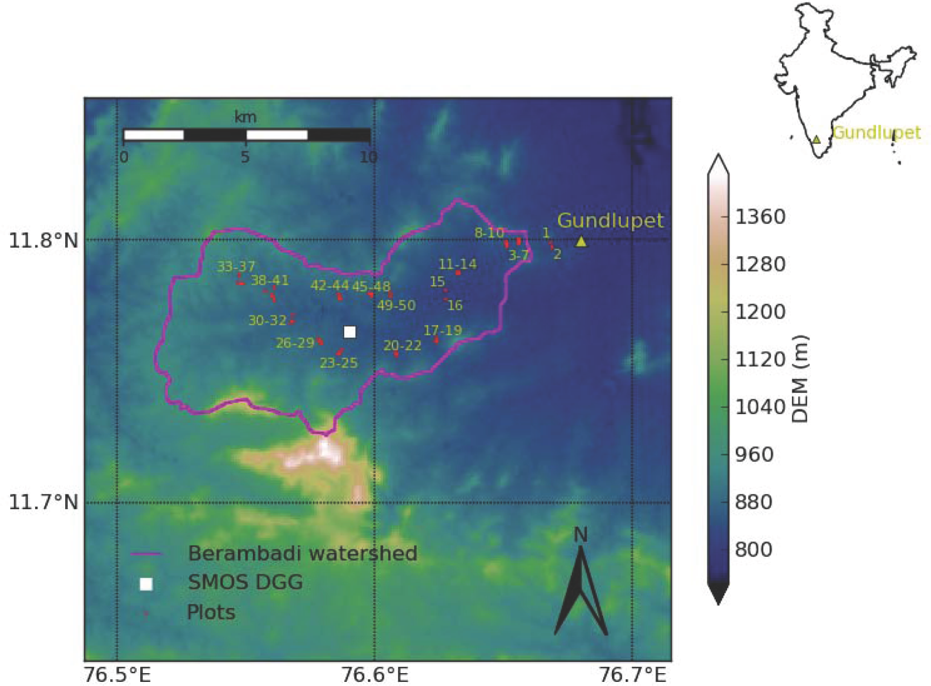
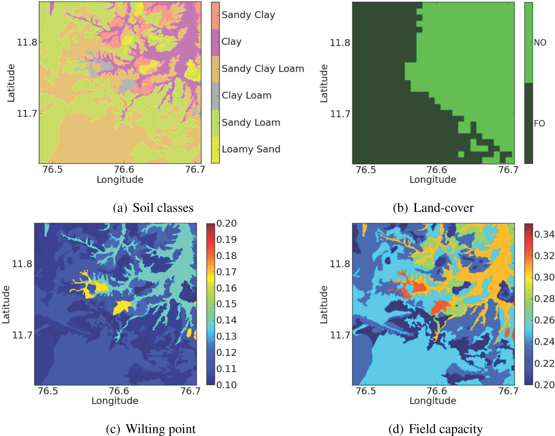
2. Study Area and Data Set
2.1. Field Data Set
2.2. Satellite Data Set
3. Methodology
3.1. SM Retrieval Models
3.2. Multi-Scale Validation of RADARSAT-2 Retrieved SM
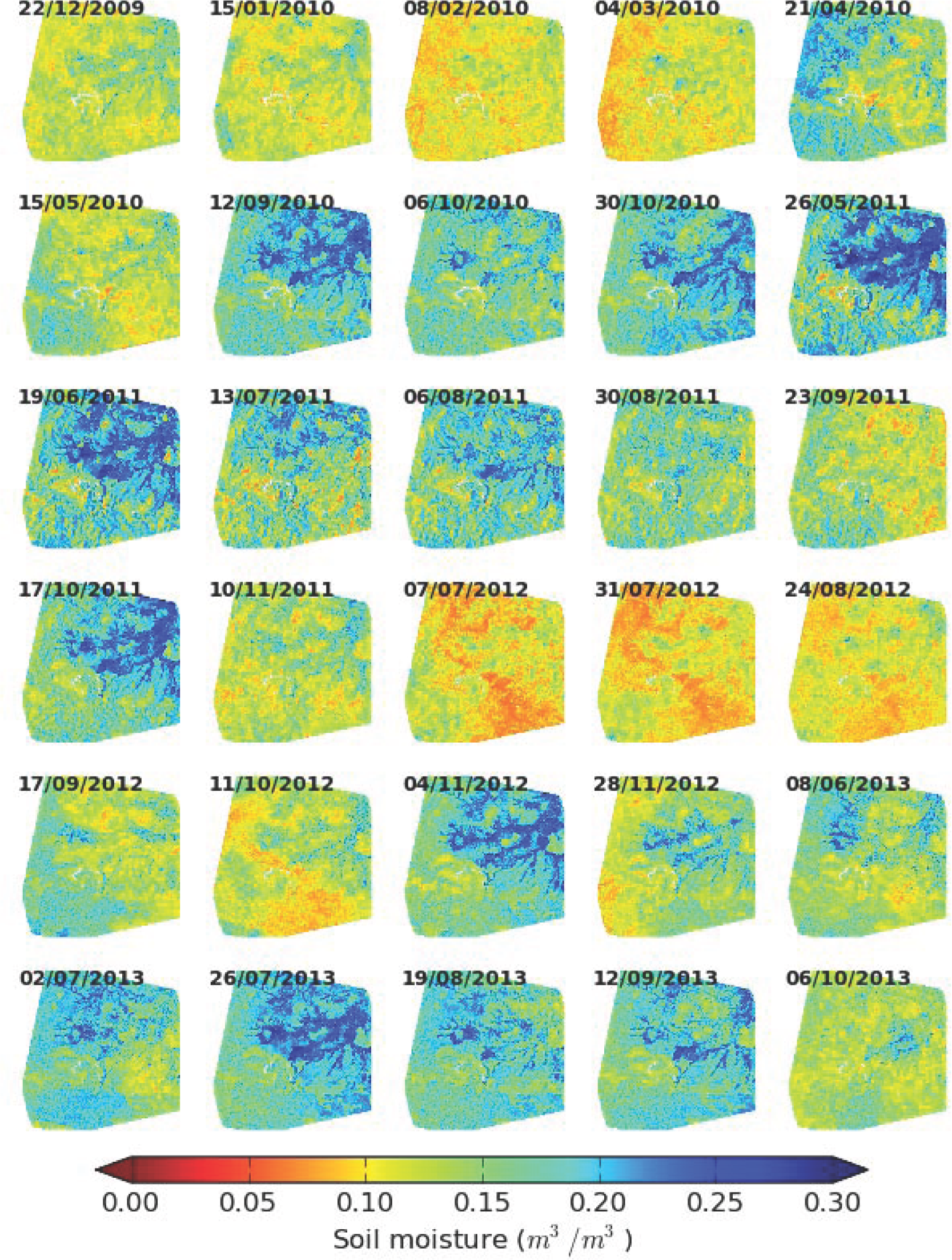
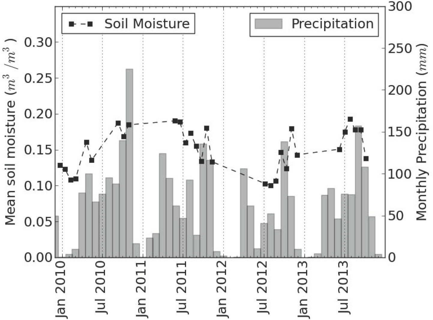
4. Results and Discussion
4.1. Results for σHH
4.2. Evaluation in terms of Data Availability
4.3. Impact of Vegetation and Roughness
4.4. Validation at SMOS Scale
5. Conclusions
Acknowledgments
Author Contributions
Conflicts of Interest
References
- Lakshmi, V. Remote sensing of soil moisture. ISRN Soil Sci. 2013. [Google Scholar] [CrossRef]
- Wood, E.F.; Roundy, J.K.; Troy, T.J.; van Beek, L.; Bierkens, M.F.; Blyth, E.; de Roo, A.; Döll, P.; Ek, M.; Famiglietti, J.; et al. Hyperresolution global land surface modeling: Meeting a grand challenge for monitoring Earth’s terrestrial water. Water Resour. Res. 2011. [Google Scholar] [CrossRef]
- Lakshmi, V. The role of satellite remote sensing in the prediction of ungauged basins. Hydrol. Process. 2004, 18, 1029–1034. [Google Scholar]
- Moran, M.S.; Peters-Lidard, C.D.; Watts, J.M.; McElroy, S. Estimating soil moisture at the watershed scale with satellite-based radar and land surface models. Can. J. Remote Sens. 2004, 30, 805–826. [Google Scholar]
- Narayan, U.; Lakshmi, V.; Jackson, T.J. High-resolution change estimation of soil moisture using L-band radiometer and radar observations made during the SMEX02 experiments. IEEE Trans. Geosci. Remote Sens. 2006, 44, 1545–1554. [Google Scholar]
- Fung, A.K.; Li, Z.; Chen, K.S. Backscattering from a randomly rough dielectric surface. IEEE Trans. Geosci. Remote Sens. 1992, 30, 356–369. [Google Scholar]
- Zribi, M.; Gorrab, A.; Baghdadi, N.; Lili-Chabaane, Z.; Mougenot, B. Influence of radar frequency on the relationship between bare surface soil moisture vertical profile and radar backscatter. IEEE Geosci. Remote Sens. Lett. 2014, 11, 848–852. [Google Scholar]
- Kelly, R.; Davie, T.; Atkinson, P. Explaining temporal and spatial variation in soil moisture in a bare field using SAR imagery. Int. J. Remote Sens. 2003, 24, 3059–3074. [Google Scholar]
- Shoshany, M.; Svoray, T.; Curran, P.J.; Foody, G.M.; Perevolotsky, A. The relation between ERS-2 SAR backscatter and soil moisture: Generalization from a humid to semi-arid transect. Int. J. Remote Sens. 2000, 21, 2337–2343. [Google Scholar]
- Sano, E.E.; Huete, A.R.; Troufleau, D.; Moran, M.S.; Vidal, A. Relation between ERS-1 synthetic aperture radar data and measurements of surface roughness and moisture content of rocky soils in a semiarid rangeland. Water Resour. Res. 1998, 34, 1491–1498. [Google Scholar]
- Paloscia, S.; Pettinato, S.; Santi, E.; Notarnicola, C.; Pasolli, L.; Reppucci, A. Soil moisture mapping using Sentinel-1 images: Algorithm and preliminary validation. Remote Sens. Environ. 2013, 134, 234–248. [Google Scholar]
- Pasolli, L.; Notarnicola, C.; Bertoldi, G.; Bruzzone, L.; Remelgado, R.; Greifeneder, F.; Niedrist, G.; Della Chiesa, S.; Tappeiner, U.; Zebisch, M. Estimation of soil moisture in mountain areas using SVR technique applied to multiscale active radar images at C-band. IEEE J. Sel. Top. Appl. Earth Obs. Remote Sens. 2015, 8, 262–283. [Google Scholar]
- Moran, M.S.; McElroy, S.; Watts, J.M.; Peters-Lidar, C. Radar remote sensing for estimation of surface soil moisture at the watershed scale. Proceedings of Modelling and Remote Sensing Applied in Agriculture (US and Mexico), Aquascalientes, Mexico, 2–6 June 2003; pp. 91–106.
- Wagner, W.; Lemoine, G.; Rott, H. A method for estimating soil moisture from ERS scatterometer and soil data. Remote Sens. Environ. 1999, 70, 191–207. [Google Scholar]
- Moran, S.; Hymer, D.; Qi, J.; Sano, E. Soil moisture evaluation using multi-temporal synthetic aperture radar (SAR) in semiarid rangeland. Agric. For. Meteorol. 2000, 105, 69–80. [Google Scholar]
- Thoma, D.; Moran, M.; Bryant, R.; Rahman, M.; Holifield-Collins, C.; Skirvin, S.; Sano, E.; Slocum, K. Comparison of four models to determine surface soil moisture from C-band radar imagery in a sparsely vegetated semiarid landscape. Water Resour. Res. 2006, 42. [Google Scholar] [CrossRef]
- Ulaby, F.T.; Moore, R.K.; Fung, A.K. Microwave Remote Sensing Active and Passive-Volume III: From Theory to Applications; Addison-Wesley: Boston, MA, USA, 1986. [Google Scholar]
- Narvekar, P.S.; Entekhabi, D.; Kim, S.B.; Njoku, E.G. Soil moisture retrieval using L-band radar observations. IEEE Trans. Geosci. Remote Sens. 2015, 53, 3492–3506. [Google Scholar]
- Mladenova, I.E.; Jackson, T.J.; Bindlish, R.; Hensley, S. Incidence angle normalization of radar backscatter data. IEEE Trans. Geosci. Remote Sens. 2013, 51, 1791–1804. [Google Scholar]
- Kottek, M.; Grieser, J.; Beck, C.; Rudolf, B.; Rubel, F. World map of the Köppen-Geiger climate classification updated. Meteorol. Z. 2006, 15, 259–263. [Google Scholar]
- Barbiéro, L.; Parate, H.R.; Descloitres, M.; Bost, A.; Furian, S.; Mohan Kumar, M.; Kumar, C.; Braun, J.J. Using a structural approach to identify relationships between soil and erosion in a semi-humid forested area, South India. Catena 2007, 70, 313–329. [Google Scholar]
- Sreelash, K.; Sekhar, M.; Ruiz, L.; Tomer, S.; Guérif, M.; Buis, S.; Durand, P.; Gascuel-Odoux, C. Parameter estimation of a two-horizon soil profile by combining crop canopy and surface soil moisture observations using GLUE. J. Hydrol. 2012, 456, 57–67. [Google Scholar]
- Sreelash, K.; Sekhar, M.; Ruiz, L.; Buis, S.; Bandyopadhyay, S. Improved modeling of groundwater recharge in agricultural watersheds using a combination of crop model and remote sensing. J. Indian Inst. Sci. 2013, 93, 189–207. [Google Scholar]
- Ahmed, N.; Mahtab, A.; Agrawal, R.; Jayaprasad, P.; Pathan, S.K.; Ajai; Singh, D.K.; Singh, A.K. Extraction and validation of Cartosat-1 DEM. J. Indian Soc. Remote Sens. 2007, 35, 121–127. [Google Scholar]
- Karnataka State Remote Sensing Application Centre. Report on State Natural Resources Information System; Technical Report; 2007; unpublished. [Google Scholar]
- Kerr, Y.H.; Waldteufel, P.; Richaume, P.; Wigneron, J.P.; Ferrazzoli, P.; Mahmoodi, A.; Al Bitar, A.; Cabot, F.; Gruhier, C.; Juglea, S.E.; et al. The SMOS soil moisture retrieval algorithm. IEEE Trans. Geosci. Remote Sens. 2012, 50, 1384–1403. [Google Scholar]
- Schaap, M.G.; Leij, F.J.; van Genuchten, M.T. rosetta: A computer program for estimating soil hydraulic parameters with hierarchical pedotransfer functions. J. Hydrol. 2001, 251, 163–176. [Google Scholar]
- Ulaby, F.T.; Moore, R.K.; Fung, A.K. Microwave Remote Sensing Active and Passive-Volume II: Radar Remote Sensing and Surface Scattering and Enission Theory; Addison-Wesley: Boston, MA, USA, 1982. [Google Scholar]
- Lievens, H.; Verhoest, N.E.; Keyser, E.D.; Vernieuwe, H.; Matgen, P.; Álvarez-Mozos, J.; Baets, B.D. Effective roughness modelling as a tool for soil moisture retrieval from C-and L-band SAR. Hydrol. Earth Syst. Sci. 2011, 15, 151–162. [Google Scholar]
- Kumar, S.; Kumar, P.; Gupta, M.; Nagawat, A. Performance comparison of median and wiener filter in image de-noising. Int. J. Comput. Appl. 2010, 12, 24–28. [Google Scholar]
- Engdahl, M.; Minchella, A.; Marinkovic, P.; Veci, L.; Lu, J. Nest: An esa open source toolbox for scientific exploitation of sar data. Proceedings of 2012 IEEE International Geoscience and Remote Sensing Symposium (IGARSS), Munich, Germany; 2012; pp. 5322–5324. [Google Scholar]
- Wang, C.; Qi, J. Biophysical estimation in tropical forests using JERS-1 SAR and VNIR imagery. II. Aboveground woody biomass. Int. J. Remote Sens. 2008, 29, 6827–6849. [Google Scholar]
- Narvekar, P.S.; Entekhabhi, D.; Kim, S.; Njoku, E. A robust algorithm for soil moisture retrieval from the Soil Moisture Active Passive mission RADAR observation. Proceedings of 2013 IEEE International Geoscience and Remote Sensing Symposium (IGARSS), Melbourne, VIC, Australia, 21–26 July 2013; pp. 45–48.
- Dubois, P.C.; Zyl, J.V.; Engman, E.T. Measuring soil moisture with imaging radars. IEEE Trans. Geosci. Remote Sens. 1995, 33, 916–926. [Google Scholar]
- Zribi, M.; Saux-Picart, S.; André, C.; Descroix, L.; Ottle, C.; Kallel, A. Soil moisture mapping based on ASAR/ENVISAT radar data over a Sahelian region. Int. J. Remote Sens. 2007, 28, 3547–3565. [Google Scholar]
- Papaefthymiou, G.; Kurowicka, D. Using copulas for modeling stochastic dependence in power system uncertainty analysis. IEEE Trans. Power Syst. 2009, 24, 40–49. [Google Scholar]
- Eilers, V.; Carter, R.; Rushton, K. A single layer soil water balance model for estimating deep drainage (potential recharge): An application to cropped land in semi-arid North-East Nigeria. Geoderma 2007, 140, 119–131. [Google Scholar]
- Silverman, B.W. Density Estimation for Statistics and Data Analysis; CRC Press: Boca Raton, FL, USA, 1986. [Google Scholar]
- Liu, Y.; Parinussa, R.; Dorigo, W.; De Jeu, R.; Wagner, W.; van Dijk, A.; McCabe, M.; Evans, J. Developing an improved soil moisture dataset by blending passive and active microwave satellite-based retrievals. Hydrol. Earth Syst. Sci. 2011, 15, 425–436. [Google Scholar]
- Al Bitar, A.; Leroux, D.; Kerr, Y.H.; Merlin, O.; Richaume, P.; Sahoo, A.; Wood, E.F. Evaluation of SMOS soil moisture products over continental US using the SCAN/SNOTEL network. IEEE Trans. Geosci. Remote Sens. 2012, 50, 1572–1586. [Google Scholar]
- Mladenova, I.; Lakshmi, V.; Walker, J.P.; Panciera, R.; Wagner, W.; Doubkova, M. Validation of the ASAR global monitoring mode soil moisture product using the NAFE’05 data set. IEEE Trans. Geosci. Remote Sens. 2010, 48, 2498–2508. [Google Scholar]
- Pathe, C.; Wagner, W.; Sabel, D.; Doubkova, M.; Basara, J. Using ENVISAT ASAR global mode data for surface soil moisture retrieval over Oklahoma, USA. IEEE Trans. Geosci. Remote Sens. 2009, 47, 468–480. [Google Scholar]
- Merlin, O.; Walker, J.P.; Panciera, R.; Escorihuela, M.J.; Jackson, T.J. Assessing the SMOS soil moisture retrieval parameters with high-resolution NAFE’06 data. IEEE Geosci. Remote Sens. Lett. 2009, 6, 635–639. [Google Scholar]
- Ulaby, F.T.; Batlivala, P.P.; Dobson, M.C. Microwave backscatter dependence on surface roughness, soil moisture and soil texture: Part I - bare soil. IEEE Trans. Geosci. Electron. 1978, GE-16, 286–295. [Google Scholar]
- Bernard, R.; Martin, P.; Thony, J.L.; Vauclin, M.; Vidal-Madjar, D. C-band radar for determining surface soil moisture. Remote Sens. Environ. 1982, 12, 189–200. [Google Scholar]
- Taconet, O.; Vidal-Madjar, D.; Emblanch, C.; Normand, M. Taking into account vegetation effects to estimate soil moisture from C-band radar measurements. Remote Sens. Environ. 1996, 56, 52–56. [Google Scholar]
- Sat Kumar; Sekhar, M.; Bandyopadhyay, S. Assimilation of remote sensing and hydrological data using adaptive filtering techniques for watershed modeling. Curr. Sci. 2009, 97, 1196–1202. [Google Scholar]
- Kim, Y.; Jackson, T.; Bindlish, R.; Lee, H.; Hong, S. Radar vegetation index for estimating the vegetation water content of rice and soybean. IEEE Geosci. Remote Sens. Lett. 2012, 9, 564–568. [Google Scholar]
- Kim, Y.; van Zyl, J. A time-series approach to estimate soil moisture using polarimetric radar data. IEEE Trans. Geosci. Remote Sens. 2009, 47, 2519–2527. [Google Scholar]
- Zribi, M.; Dechambre, M. A new empirical model to retrieve soil moisture and roughness from C-band radar data. Remote Sens. Environ. 2003, 84, 42–52. [Google Scholar]
- Álvarez-Mozos, J.; Verhoest, N.; Larrañaga, A.; Casalí, J.; González-Audícana, M. Influence of surface roughness spatial variability and temporal dynamics on the retrieval of soil moisture from SAR observations. Sensors 2009, 9, 463–489. [Google Scholar]
- Jackson, T.; McNairn, H.; Weltz, M.; Brisco, B.; Brown, R. First order surface roughness correction of active microwave observations for estimating soil moisture. IEEE Trans. Geosci. Remote Sens. 1997, 35, 1065–1069. [Google Scholar]
- Turner, R.; Panciera, R.; Tanase, M.A.; Lowell, K.; Hacker, J.M.; Walker, J.P. Estimation of soil surface roughness of agricultural soils using airborne LiDAR. Remote Sens. Environ. 2014, 140, 107–117. [Google Scholar]
- Gherboudj, I.; Magagi, R.; Berg, A.; Toth, B. Soil moisture retrieval over agricultural fields from multi-polarized and multi-angular RADARSAT-2 SAR data. Remote Sens. Environ. 2011, 115, 33–43. [Google Scholar]
- Zribi, M.; Chahbi, A.; Shabou, M.; Lili-Chabaane, Z.; Duchemin, B.; Baghdadi, N.; Amri, R.; Chehbouni, A. Soil surface moisture estimation over a semi-arid region using ENVISAT ASAR radar data for soil evaporation evaluation. Hydrol. Earth Syst. Sci. Discuss. 2011, 15, 345–358. [Google Scholar]
- Le Morvan, A.; Zribi, M.; Baghdadi, N.; Chanzy, A. Soil moisture profile effect on radar signal measurement. Sensors 2008, 8, 256–270. [Google Scholar]
- Álvarez-Mozos, J.; Casalí, J.; González-Audícana, M.; Verhoest, N.E. Assessment of the operational applicability of RADARSAT-1 data for surface soil moisture estimation. IEEE Trans. Geosci. Remote Sens. 2006, 44, 913–924. [Google Scholar]
- Dobson, M.C.; Ulaby, F.T. Active microwave soil moisture research. IEEE Trans. Geosci. Remote Sens. 1986, GE-24, 23–36. [Google Scholar]
- Lawrence, H.; Wigneron, J.P.; Richaume, P.; Novello, N.; Grant, J.; Mialon, A.; Al Bitar, A.; Merlin, O.; Guyon, D.; Leroux, D.; et al. Comparison between SMOS Vegetation Optical Depth products and MODIS vegetation indices over crop zones of the USA. Remote Sens. Environ. 2014, 140, 396–406. [Google Scholar]
- Rahmoune, R.; Ferrazzoli, P.; Singh, Y.; Kerr, Y.; Richaume, P.; Al Bitar, A. SMOS retrieval results over forests: Comparisons with independent measurements. IEEE J. Sel. Top. Appl. Earth Obs. Remote Sens. 2014, 7, 3858–3866. [Google Scholar]
- Kerr, Y.H.; Waldteufel, P.; Wigneron, J.P.; Martinuzzi, J.; Font, J.; Berger, M. Soil moisture retrieval from space: The Soil Moisture and Ocean Salinity (SMOS) mission. IEEE Trans. Geosci. Remote Sens. 2001, 39, 1729–1735. [Google Scholar]
- Raju, S.; Chanzy, A.; Wigneron, J.P.; Calvet, J.C.; Kerr, Y.; Laguerre, L. Soil moisture and temperature profile effects on microwave emission at low frequencies. Remote Sens. Environ. 1995, 54, 85–97. [Google Scholar]
- Escorihuela, M.J.; Chanzy, A.; Wigneron, J.P.; Kerr, Y. Effective soil moisture sampling depth of L-band radiometry: A case study. Remote Sens. Environ. 2010, 114, 995–1001. [Google Scholar]
- McCabe, M.; Gao, H.; Wood, E. Evaluation of AMSR-E-derived soil moisture retrievals using ground-based and PSR airborne data during SMEX02. J. Hydrometeorol. 2005, 6, 864–877. [Google Scholar]
- Mladenova, I.; Lakshmi, V.; Jackson, T.J.; Walker, J.P.; Merlin, O.; de Jeu, R.A.M. Validation of AMSR-E soil moisture using L-band airborne radiometer data from National Airborne Field Experiment 2006. Remote Sens. Environ. 2011, 115, 2096–2103. [Google Scholar]
- Qiu, J.; Crow, W.T.; Nearing, G.S.; Mo, X.; Liu, S. The impact of vertical measurement depth on the information content of soil moisture times series data. Geophys. Res. Lett. 2014, 41, 4997–5004. [Google Scholar]
- Bizzarri, B.; Wigneron, J.P.; Kerr, Y. Operational readiness of microwave remote sensing of soil moisture for hydrologic applications. Nord. Hydrol. 2007, 38, 1–20. [Google Scholar]
- Al-Yaari, A.; Wigneron, J.P.; Ducharne, A.; Kerr, Y.; de Rosnay, P.; de Jeu, R.; Govind, A.; Al Bitar, A.; Albergel, C.; Muñoz-Sabater, J.; et al. Global-scale evaluation of two satellite-based passive microwave soil moisture datasets (SMOS and AMSR-E) with respect to Land Data Assimilation System estimates. Remote Sens. Environ. 2014, 149, 181–195. [Google Scholar]


| Year | Date/Month | Pixel Spacing (m) | Line Spacing (m) | Beam Mode | Pass Direction | Incidence Angle (degree) |
|---|---|---|---|---|---|---|
| 2009 | 22/12 | 4.73 | 5.33 | FQ3 | Ascending | 20 |
| 2010 | 15/01, 08/02, 04/03, 21/04, 15/05, 12/09, 06/10, 30/10 | 4.73 | 5.33 | FQ3 | Ascending | 20 |
| 2011 | 26/05, 19/06, 13/07, 06/08, 30/08, 23/09, 14/10, 10/11 | 4.73 | 4.70 | FQ6 | Descending | 23 |
| 2012 | 07/07, 31/07, 24/08, 17/09, 11/10, 04/11, 28/11 | 4.73 | 4.70 | FQ6 | Descending | 24 |
| 2013 | 08/06, 02/07, 26/07, 19/08, 12/09, 06/10 | 4.73 | 4.70 | FQ6 | Descending | 25 |
| S.N. | Mean Antenna Footprint | Land Cover | Soil Texture |
|---|---|---|---|
| 1 | 1 | 1 | 1 |
| 2 | 0.48–1.0 | 1 | 1 |
| 3 | 1 | 0–1 | 1 |
| 4 | 0.48–1.0 | 0–1 | 1 |
| 5 | 1 | 1 | 0.08–0.56 |
| 6 | 0.48–1.0 | 1 | 0.08–0.56 |
| 7 | 1 | 0 – 1 | 0.08–0.56 |
| 8 | 0.48–1.0 | 0–1 | 0.08–0.56 |
| Plot # | n | R | RMSE | Bias | Plot # | n | R | RMSE | Bias |
|---|---|---|---|---|---|---|---|---|---|
| 1 | 23 | 0.77 | 0.05 | −0.03 | 26 | 28 | 0.61 | 0.08 | −0.01 |
| 2 | 17 | 0.72 | 0.05 | −0.03 | 27 | 27 | 0.64 | 0.07 | −0.04 |
| 3 | 28 | 0.11 | 0.11 | 0.04 | 28 | 28 | 0.66 | 0.08 | −0.04 |
| 4 | 28 | 0.28 | 0.06 | −0.02 | 29 | 27 | 0.61 | 0.11 | 0.06 |
| 5 | 26 | 0.25 | 0.07 | −0.04 | 30 | 28 | 0.62 | 0.10 | 0.06 |
| 6 | 27 | 0.45 | 0.06 | −0.03 | 31 | 28 | 0.60 | 0.08 | 0.03 |
| 7 | 27 | 0.57 | 0.07 | −0.05 | 32 | 19 | 0.63 | 0.16 | 0.13 |
| 8 | 28 | 0.74 | 0.06 | −0.05 | 33 | 26 | 0.71 | 0.06 | 0.00 |
| 9 | 28 | 0.67 | 0.05 | −0.04 | 34 | 26 | 0.67 | 0.07 | 0.03 |
| 10 | 27 | 0.54 | 0.06 | −0.04 | 35 | 24 | 0.65 | 0.09 | 0.04 |
| 11 | 25 | 0.30 | 0.07 | −0.04 | 36 | 26 | 0.67 | 0.09 | 0.06 |
| 12 | 26 | 0.60 | 0.07 | −0.05 | 37 | 26 | 0.71 | 0.05 | −0.02 |
| 13 | 28 | 0.50 | 0.07 | −0.04 | 38 | 19 | 0.70 | 0.07 | 0.00 |
| 14 | 27 | 0.42 | 0.08 | −0.06 | 39 | 26 | 0.54 | 0.11 | 0.06 |
| 15 | 26 | 0.68 | 0.09 | 0.03 | 40 | 26 | 0.74 | 0.08 | 0.04 |
| 16 | 28 | 0.39 | 0.09 | 0.03 | 41 | 26 | 0.67 | 0.05 | 0.01 |
| 17 | 25 | 0.66 | 0.08 | −0.06 | 42 | 24 | 0.55 | 0.08 | 0.02 |
| 18 | 28 | 0.47 | 0.08 | −0.06 | 43 | 26 | 0.40 | 0.08 | 0.00 |
| 19 | 28 | 0.30 | 0.11 | −0.02 | 44 | 25 | 0.39 | 0.07 | 0.01 |
| 20 | 27 | 0.61 | 0.07 | −0.05 | 45 | 25 | 0.55 | 0.07 | 0.00 |
| 21 | 28 | 0.52 | 0.08 | 0.04 | 46 | 12 | 0.48 | 0.06 | −0.02 |
| 22 | 28 | 0.49 | 0.08 | 0.05 | 47 | 11 | 0.95 | 0.03 | −0.03 |
| 23 | 28 | 0.28 | 0.10 | 0.03 | 48 | 12 | 0.61 | 0.05 | −0.03 |
| 24 | 28 | 0.45 | 0.11 | 0.07 | 49 | 25 | 0.80 | 0.04 | −0.01 |
| 25 | 28 | 0.55 | 0.10 | 0.03 | 50 | 25 | 0.69 | 0.06 | 0.00 |
© 2015 by the authors; licensee MDPI, Basel, Switzerland This article is an open access article distributed under the terms and conditions of the Creative Commons Attribution license (http://creativecommons.org/licenses/by/4.0/).
Share and Cite
Tomer, S.K.; Al Bitar, A.; Sekhar, M.; Zribi, M.; Bandyopadhyay, S.; Sreelash, K.; Sharma, A.K.; Corgne, S.; Kerr, Y. Retrieval and Multi-scale Validation of Soil Moisture from Multi-temporal SAR Data in a Semi-Arid Tropical Region. Remote Sens. 2015, 7, 8128-8153. https://doi.org/10.3390/rs70608128
Tomer SK, Al Bitar A, Sekhar M, Zribi M, Bandyopadhyay S, Sreelash K, Sharma AK, Corgne S, Kerr Y. Retrieval and Multi-scale Validation of Soil Moisture from Multi-temporal SAR Data in a Semi-Arid Tropical Region. Remote Sensing. 2015; 7(6):8128-8153. https://doi.org/10.3390/rs70608128
Chicago/Turabian StyleTomer, Sat Kumar, Ahmad Al Bitar, Muddu Sekhar, Mehrez Zribi, S. Bandyopadhyay, K. Sreelash, A.K. Sharma, Samuel Corgne, and Yann Kerr. 2015. "Retrieval and Multi-scale Validation of Soil Moisture from Multi-temporal SAR Data in a Semi-Arid Tropical Region" Remote Sensing 7, no. 6: 8128-8153. https://doi.org/10.3390/rs70608128
APA StyleTomer, S. K., Al Bitar, A., Sekhar, M., Zribi, M., Bandyopadhyay, S., Sreelash, K., Sharma, A. K., Corgne, S., & Kerr, Y. (2015). Retrieval and Multi-scale Validation of Soil Moisture from Multi-temporal SAR Data in a Semi-Arid Tropical Region. Remote Sensing, 7(6), 8128-8153. https://doi.org/10.3390/rs70608128