
A Dynamic Vegetation Senescence Indicator for Near-Real-Time Desert Locust Habitat Monitoring with MODIS


 ,
,
Abstract
:
1. Introduction
2. Material
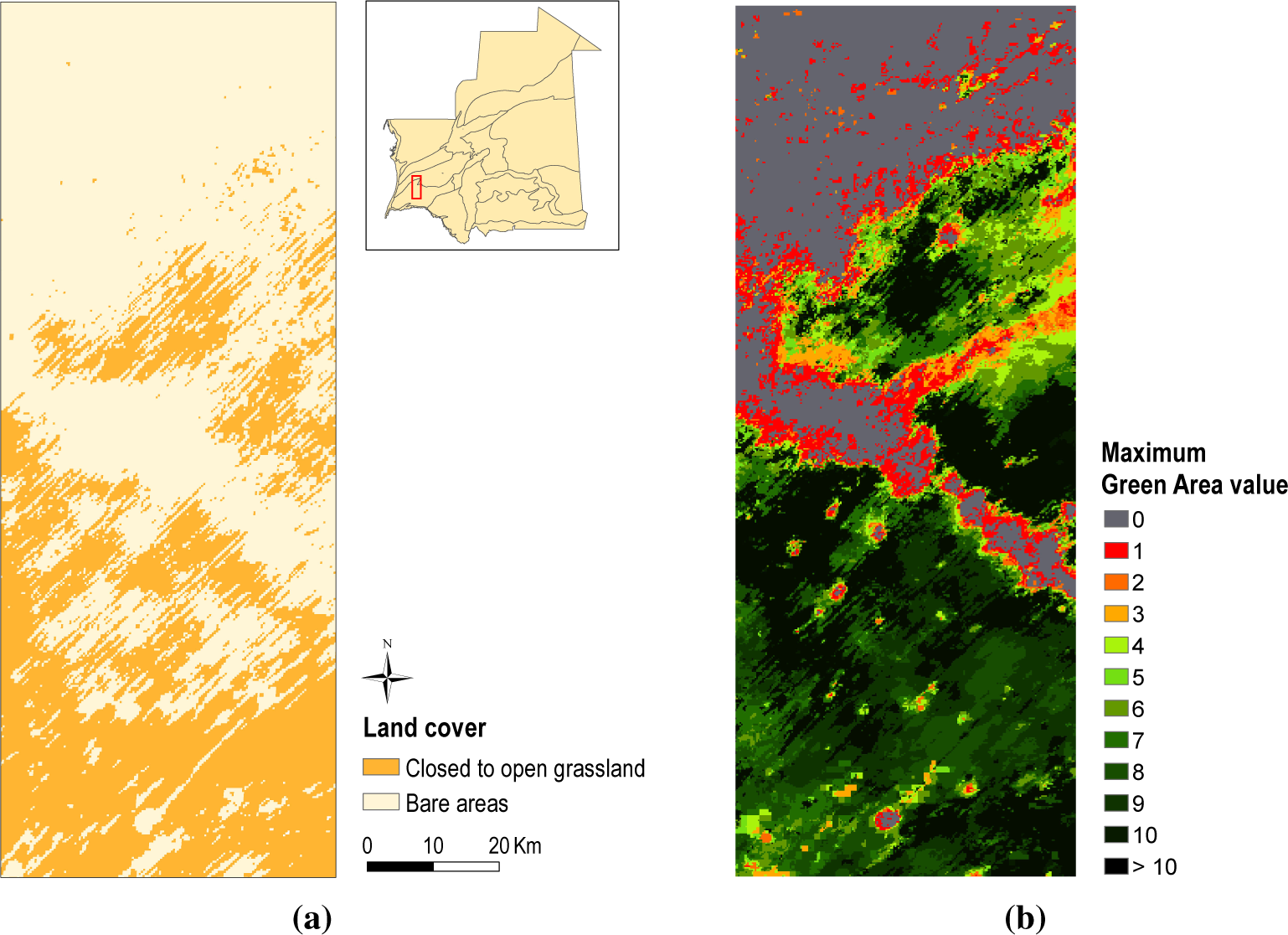
2.1. Study Site
2.2. Data Sources
3. Methodology
3.1. Rationale
3.2. Data Preprocessing
3.2.1. Field Observation Preprocessing
- Growth: the observation was located on the increasing part of the NDVI curve and was designated as “green” in the database RAMSES;
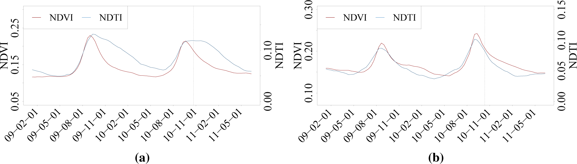
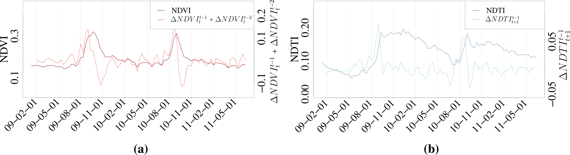
- Drying: the observation was reported as “drying” in RAMSES and was located on the decreasing part of the NDVI curve while the NDTI curve remained stable (i.e., presence of a stall point). There was no apparent decrease of the vegetation cover and the vegetation shifted from a “green” state to a “drying” state. The NDTI remained constant before entering a decrease phase due to the vegetation degradation;
- Density reduction: the observation was described as “green” or “drying” in RAMSES and was on the decreasing part of the NDVI and NDTI curves. As NDTI is sensitive to both green and dry vegetation, a decrease in its temporal trajectory indicates a reduction of vegetation. This class does not exclude the two others, but in this case, the actual state of the vegetation remained undetermined (likely drying). Caution should be taken in the interpretation of the errors of the classification of this class.
3.2.2. Remote Sensing Data Preprocessing
3.3. Senescence Detection and Dynamic Mapping
3.3.1. Metric Definition and Selection
3.3.2. Classification Methods and Accuracy Assessment
3.4. Near-Real-Time Simulation Study Case
4. Results and Discussion
4.1. Metric Evaluation
4.2. Classification Benchmarking
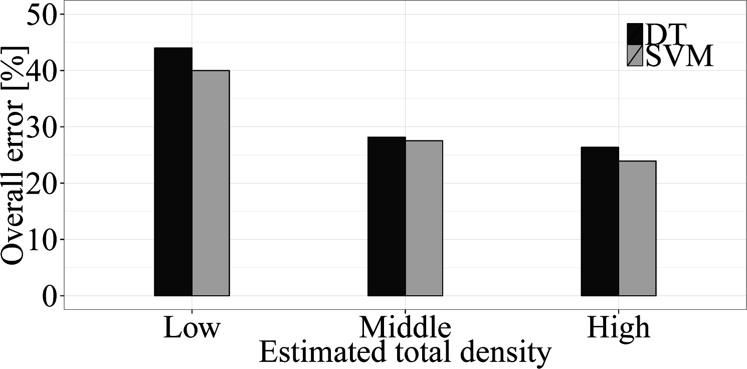
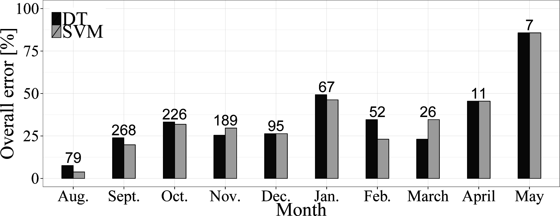
4.3. Analysis of the Error
4.4. Near-Real-Time Dynamic Dryness Mapping Case Study
5. Conclusions
Acknowledgments
Author Contributions
Conflicts of Interest
References
- Duranton, J.F.; Lecoq, M. Le Criquet Pèlerin au Sahel; Comité permanent inter-etats de lutte contre la sécheresse au Sahel: Ouagadougou, Brukina Faso, 1990. [Google Scholar]
- Ould Baba, M. Biogéographie du Criquet pèlerin en Mauritanie, Fonctionnement d’une Aire Grégarigène et Conséquences sur L’organisation de la Surveillance et de la Lutte Anti-acridienne. Master Thesis, École Pratique des Hautes Études, FAO, Rome, Italy, 2001. [Google Scholar]
- Cressman, K. Dynamic Greenness Maps, a Brief Report on Usage for Desert Locust Early Warning; Technical Report May, Desert Locust Information Service; FAO: Rome, Italy, 2012. [Google Scholar]
- Brader, L.; Djibo, H.; Faye, F.G.; Babah, M.A.O.; Ghaout, S.; Lazar, P.M.; Nguala, M. Towards a More Effective Response to Desert Locusts and Their Impacts on Food Security, Livelihood and Poverty. Independent Multilateral Evaluation of the 2003–2005 Desert Locust Campaign; Technical Report July; FAO: Rome, Italy, 2006. [Google Scholar]
- De Vreyer, P.; Guilbert, N.; Mesplé-Somps, S. The 1987–1989 Locust Plague in Mali: Evidences of the Heterogeneous Impact of Income Shocks on Education Outcomes; Université Paris-Dauphine: Paris, France, 2012. [Google Scholar]
- Uvarov, B.P. Grasshoppers and Locusts: A Handbook of General Acridology. vol. 1. Anatomy, Physiology, Development, Phase Polymorphism, Introduction to Taxonomy; Anti-Locust Research Centre at the University Press: London, UK, 1966. [Google Scholar]
- Roffey, J.; Popov, G. Environmental and behavioural processes in a desert locust outbreak. Nature 1968, 219, 446–450. [Google Scholar]
- Hay, S.I. Remote sensing and disease control: Past, present and future. Trans. R. Soc. Trop. Med. Hyg 1997, 91, 105–106. [Google Scholar]
- Culmsee, H. Etudes sur le Comportement Alimentaire et Migratoire du Criquet pelerin Schistocerca Gregaria en Fonction de la Végétation en Mauritanie; Technical Report, Projekt Biologisch-Integrierte Heuschreckenbekämpfung; Deutsche Gesellschaft für Technische Zusammenarbeit: Eschborn, Germany, 1997. [Google Scholar]
- Ghaout, S. Contribution à L’étude des Ressources Trophiques de Schistocerca Gregaria (Forskal, 1775) (Orthoptera, Acrididae) Solitaire en Mauritanie Occidentale et Télédétection de ses Biotopes par Satellite. Ph.D Thesis, Université Paris XI, Orsay, France, 1990; p. 241. [Google Scholar]
- El Hadj, A. Biologie et écologie de Schistocerca gregaria (Forskål)(Orthoptera: Acrididae) et de ses plantes-hôtes en Mauritanie: Effets des triterpènes de Citrullus colocynthis (Schrader). Ph.D Thesis, Université Mohammed V, Rabbat, Morocco, 1997. [Google Scholar]
- Despland, E.; Simpson, S. The role of food distribution and nutritional quality in behavioural phase change in the desert locust. Anim. Behav 2000, 59, 643–652. [Google Scholar]
- El-Bashir, S. Stratégies d’adaptation et de survie du Criquet pèlerin dans un milieu de récession et de multiplication. Sécheresse 1996, 7, 115–118. [Google Scholar]
- Ellis, P.E.; Ashall, C. Field Studies on diurnal Behaviour, Movement and Aggregation in the Desert Locust (Schistocerca gregaria Forskål). Anti-Locust Bull 1957, 25, 4–84. [Google Scholar]
- Kennedy, J. The behaviour of the desert locust (Schistocerca gregaria (Forsk.)) (Orthoptera) in an outbreak centre. Tran. R. Entomol. Soc. Lond 1939, 89, 385–542. [Google Scholar]
- Cressman, K. Monitoring desert locusts in the Middle East : An overview. In Transformations of Middle Eastern Natural Environnements : Legacies ans Lessons; Coppock, J., Miller, J.A., Albert, J., Bernhardsson, M., Kenna, R., Eds.; Yale School of Forestry and Environmental Studies: New Haven, CT, USA, 1998; p. 492. [Google Scholar]
- Lecoq, M. Desert locust threat to agricultural development and food security and FAO/International role in its control. Arab J. Plant Protect 2003, 21, 188–193. [Google Scholar]
- Van Huis, A.; Cressman, K.; Magor, J.I. Preventing desert locust plagues: optimizing management interventions. Entomol. Exp. Appl 2007, 122, 191–214. [Google Scholar]
- Cossée, O.; Lazar, M.; Hassane, S. Rapport de l’évaluation à mi-parcours du Programme EMPRES Composante Criquet pèlerin en Région Occidentale; Technical Report for FAO; Rome, Italy, 2009. [Google Scholar]
- Lecoq, M. Vers une solution durable au problème du criquet pèlerin. Sécheresse 2004, 15, 217–224. [Google Scholar]
- Hielkema, J. Application of Landsat Data in Desert Locust Survey and Control: Desert Locust Satellite Application Project, Stage II; FAO: Rome, Italy, 1977. [Google Scholar]
- Hielkema, J.U.; Roffey, J.; Tucker, C.J. Assessment of ecological conditions associated with the 1980/81 desert locust plague upsurge in West Africa using environmental satellite data. Int. J. Remote Sens 1986, 7, 1609–1622. [Google Scholar]
- Pedgley, D. Testing feasibility of detecting locust breeding sites by satellite; Final Report to NASA on ERTS-1 Experiment; COPR: London, UK, 1973. [Google Scholar]
- Sinha, P.; Chandra, S. Visual analysis of land satellite imageries with references to growth and decay of vegetation in Western Rajasthan. Plant Protect. Bull 1987, 39, 29–31. [Google Scholar]
- Steinbauer, M.J. Relating rainfall and vegetation greenness to the biology of spur-throated and Australian plague locusts. Agric. For. Entomol 2011, 13, 205–218. [Google Scholar]
- Tappan, G.G.; Moore, D.G.; Knausenberger, W.I. Monitoring grasshopper and locust habitats in Sahelian Africa using GIS and remote sensing technologyâẶă. Int. J. Geogr. Inf. Syst 1991, 5, 123–135. [Google Scholar]
- Despland, E.; Rosenberg, J.; Simpson, S.J. Landscape structure and locust swarming : A satellite’s eye view. Ecography 2004, 3, 381–391. [Google Scholar]
- Cherlet, M.; Mathoux, P.; Bartholomé, E.; Defourny, P. Spot vegetation contribution to desert locust habitat monitoring. Proceedings of the VEGETATION 2000 Workshop, Lake Maggiore, Italy, 3–6 April 2000.
- Ceccato, P. Operational early warning system using SPOT-VGT and TERRA-MODIS to predict desert locust outbreaks. Proceedings of the 2nd VEGETATION International Users Conference, Antwerpen, Belgium, 24–26 March 2004; 2005; pp. 24–26. [Google Scholar]
- Pekel, J.F.; Ceccato, P.; Vancutsem, C.; Cressman, K.; Vanbogaert, E.; Defourny, P. Development and application of multi-temporal colorimetric transformation to monitor vegetation in the desert locust habitat. IEEE J. Sel. Top. Appl. Earth Obs. Remote Sens 2010, 9, 1939–1404. [Google Scholar]
- Cressman, K. The use of new technologies in Desert Locust early warning. Outlooks Pest Manag 2008, 19, 55–59. [Google Scholar]
- Waldner, F.; Babah Ebbe, M.; Cressman, K.; Defourny, P. Operational monitoring of the Desert Locust habitat with Earth Observation: An assessment. Int. J. Appl. Earth Obs. Geoinf Submitted. 2015. [Google Scholar]
- Jacques, D.C.; Kergoat, L.; Hiernaux, P.; Mougin, E.; Defourny, P. Monitoring dry vegetation masses in semi-arid areas with MODIS SWIR bands. Remote Sens. Environ 2014, 153, 40–49. [Google Scholar]
- Kergoat, L.; Hiernaux, P.; Dardel, C.; Pierre, C.; Guichard, F.; Kalilou, A. Dry-season vegetation mass and cover fraction from SWIR1. 6 and SWIR2. 1 band ratio: Ground-radiometer and MODIS data in the Sahel. Int. J. Appl. Earth Obs. Geoinf 2015, 39, 56–64. [Google Scholar]
- Marsett, R.; Qi, J.; Heilman, P.; Biedenbender, S.; Watson, M.; Amer, S.; Weltz, M.; Goodrich, D.; Marsett, R. Remote sensing for grassland management in the arid southwest. Rangel. Ecol. Manag 2006, 59, 530–540. [Google Scholar]
- Serbin, G.; Hunt, E.; Daughtry, C.; McCarty, G.; Doraiswamy, P. An improved ASTER index for remote sensing of crop residue. Remote Sens 2009, 1, 971–991. [Google Scholar]
- Zheng, B.; Campbell, J.B.; de Beurs, K.M. Remote sensing of crop residue cover using multi-temporal Landsat imagery. Remote Sens. Environ 2012, 117, 177–183. [Google Scholar]
- Daughtry, C.; Doraiswamy, P.; Hunt, E.; Stern, A.; McMurtrey, J., III; Prueger, J. Remote sensing of crop residue cover and soil tillage intensity. Soil Tillage Res 2006, 91, 101–108. [Google Scholar]
- Guerschman, J.; Hill, M.J.; Renzullo, L.J.; Barrett, D.J.; Marks, A.S.; Botha, E.J. Estimating fractional cover of photosynthetic vegetation, non-photosynthetic vegetation and bare soil in the Australian tropical savanna region upscaling the EO-1 Hyperion and MODIS sensors. Remote Sens. Environ 2009, 113, 928–945. [Google Scholar]
- Monty, J.; Daughtry, C.; Crawford, M. Assessing crop residue cover using hyperion data. Proceedings of the IEEE International Geoscience and Remote Sensing Symposium 2008 (IGARSS 2008), Boston, MA, USA, 7–11 July 2008; 2, pp. II-303–II-303.
- Roberts, D.; Dennison, P.; Gardner, M.; Hetzel, Y.; Ustin, S.; Lee, C. Evaluation of the potential of Hyperion for fire danger assessment by comparison to the Airborne Visible/Infrared Imaging Spectrometer. IEEE Trans. Geosci. Remote Sens 2003, 41, 1297–1310. [Google Scholar]
- Hiernaux, P.; Mougin, E.; Diawara, M.; Soumaguel, N.; Diarra, L. How Much does Grazing Contribute to Herbaceous Decay during the Dry Season in Sahel Rangelands? Technical Report for Elevage Climat Société; Agence Nationale de la Recherche: Paris, France, 2013. [Google Scholar]
- Grouzis, M. Structure, Productivité, et Dynamique des Systèmes Écologiques Sahéliens (Mare d’Oursi, Burkina Faso). Ph.D Thesis, Université de Paris Sud, Paris, France, 1988. [Google Scholar]
- Jaavar, B. Contribution à l’étude descriptive et causale de la chorologie du Criquet pélerin (Schistocerca gregaria Forskål, 1775) en Mauritanie; Ministére de L’enseignement Supérieur et de la Recherche: Paris, France, 2011. [Google Scholar]
- Vancutsem, C.; Pekel, J.F.; Bogaert, P.; Defourny, P. Mean Compositing, an alternative strategy for producing temporal syntheses. Concepts and performance assessment for SPOT VEGETATION time series. Int. J. Remote Sens 2007, 28, 5123–5141. [Google Scholar]
- Daughtry, C.S.T.; Hunt, E.R.; Doraiswamy, P.C.; McMurtrey, J.E. Remote sensing the spatial distribution of crop residues. Agron. J. 2005, 97, 864. [Google Scholar]
- Daughtry, C.; Hunt, E., Jr. Mitigating the effects of soil and residue water contents on remotely sensed estimates of crop residue cover. Remote Sens. Environ 2008, 112, 1647–1657. [Google Scholar]
- Arsenault, E.; et Bonn, F. Evaluation of soil erosion protective cover by crop residues using vegetation indices and spectral mixture analysis of multispectral and hyperspectral data. Catena 2005, 62, 157–172. [Google Scholar]
- Biard, F.; Baret, F. Crop residue estimation using multiband reflectance. Remote Sens. Environ 1997, 59, 530–536. [Google Scholar]
- Bannari, A.; Chevrier, M.; Staenz, K.; McNairn, H. Potential of hyperspectral indices for estimating crop residue cover. Revue Télédétect 2007, 7, 447–463. [Google Scholar]
- Bergeron, M. Caractérisation du Recouvrement végétal et des Pratiques Agricoles à L’aide D’une Image TM Landsat au Nord du Viêt Nam. Ph.D Thesis, Université de Sherbrooke, Sherbrooke, QC, Canada, 2000. [Google Scholar]
- Cao, X.; Chen, J.; Matsushita, B.; Imura, H. Developing a MODIS-based index to discriminate dead fuel from photosynthetic vegetation and soil background in the Asian steppe area. Int. J. Remote Sens 2010, 31, 1589–1604. [Google Scholar]
- Elmore, A.J.; Asner, G.P.; Hughes, R.F. Satellite monitoring of vegetation phenology and fire fuel conditions in hawaiian drylands. Earth Interact 2005, 9, 1–21. [Google Scholar]
- Peña-Barragán, J.M.; Ngugi, M.K.; Plant, R.E.; Six, J. Object-based crop identification using multiple vegetation indices, textural features and crop phenology. Remote Sens. Environ 2011, 115, 1301–1316. [Google Scholar]
- Van Deventer, A.; Ward, A.; Gowda, P.; Lyon, J. Using Thematic Mapper data to identify contrasting soil plains and tillage practices. PE RS- Photogramm. Eng. Remote Sens 1997, 63, 87–93. [Google Scholar]
- Popov, G.; Duranton, J.F.; Gigault. Locust Handbook; CIRAD, PRIFAS, Acridologie Opérationnelle: Montpellier, France, 1991; p. 743. [Google Scholar]
- Atkinson, P.M.; Jeganathan, C.; Dash, J.; Atzberger, C. Inter-comparison of four models for smoothing satellite sensor time-series data to estimate vegetation phenology. Remote Sens. Environ 2012, 123, 400–417. [Google Scholar]
- Eilers, P.H.C. A perfect smoother. Anal. Chem 2003, 75, 3631–3636. [Google Scholar]
- Fawcett, T. An introduction to ROC analysis. Pattern Recognit. Lett 2006, 27, 861–874. [Google Scholar]
- Bradley, A.P. The use of the area under the ROC curve in the evaluation of machine learning algorithms. Pattern Recognit 1997, 30, 1145–1159. [Google Scholar]
- Landgrebe, D. Signal Theory Method in Multispectral Remote Sensing; Wiley: Hoboken, NJ, USA, 2003; p. 508. [Google Scholar]
- Ahmad, A.; Quegan, S. Analysis of maximum likelihood classification on multispectral data. Appl. Math. Sci 2012, 6, 6425–6436. [Google Scholar]
- Xu, M.; Watanachaturaporn, P.; Varshney, P.; Arora, M. Decision tree regression for soft classification of remote sensing data. Remote Sens. Environ 2005, 97, 322–336. [Google Scholar]
- Pal, M.; Mather, P.M. An assessment of the effectiveness of decision tree methods for land cover classification. Remote Sens. Environ 2003, 86, 554–565. [Google Scholar]
- Gahegan, M.; West, G. The classification of complex geographic datasets: An operational comparison of artificial neural network and decision tree classifiers. Procedings of the Third International Conference on GeoComputation, Bristol, UK, 17–19 September 1998; pp. 17–19.
- Huang, C.; Davis, L.S.; Townshend, J.R.G. An assessment of support vector machines for land cover classification. Int. J. Remote Sens 2002, 23, 725–749. [Google Scholar]
- Gualtieri, J.A.; Cromp, R.F. Support Vector Machines for Hyperspectral Remote Sensing Classification. Proc. SPIE 1999. [Google Scholar] [CrossRef]
- Boschetti, L.; Flasse, S.P.; Brivio, P.A. Analysis of the conflict between omission and commission in low spatial resolution dichotomic thematic products: The Pareto Boundary. Remote Sens. Environ 2004, 91, 280–292. [Google Scholar]
- Babah, M.A.O.; Sword, G.A. Linking locust gregarization to local resource distribution patterns across a large spatial scale. Environ. Entomol 2004, 33, 1577–1583. [Google Scholar]


 “growth”,
 “density reduction” and
 “drying” every 10-day from the 21/07/2010 to the 21/01/2011 (a–s). Map (t) summarizes the dynamic dryness status at the end of the second 10-day interval of October. It highlights areas less suitable for desert locusts (in grey and yellow scales).
“growth”,
“density reduction” and
“drying” every 10-day from the 21/07/2010 to the 21/01/2011 (a–s). Map (t) summarizes the dynamic dryness status at the end of the second 10-day interval of October. It highlights areas less suitable for desert locusts (in grey and yellow scales).
“drying” every 10-day from the 21/07/2010 to the 21/01/2011 (a–s). Map (t) summarizes the dynamic dryness status at the end of the second 10-day interval of October. It highlights areas less suitable for desert locusts (in grey and yellow scales).
“growth”,
“density reduction” and
“drying” every 10-day from the 21/07/2010 to the 21/01/2011 (a–s). Map (t) summarizes the dynamic dryness status at the end of the second 10-day interval of October. It highlights areas less suitable for desert locusts (in grey and yellow scales).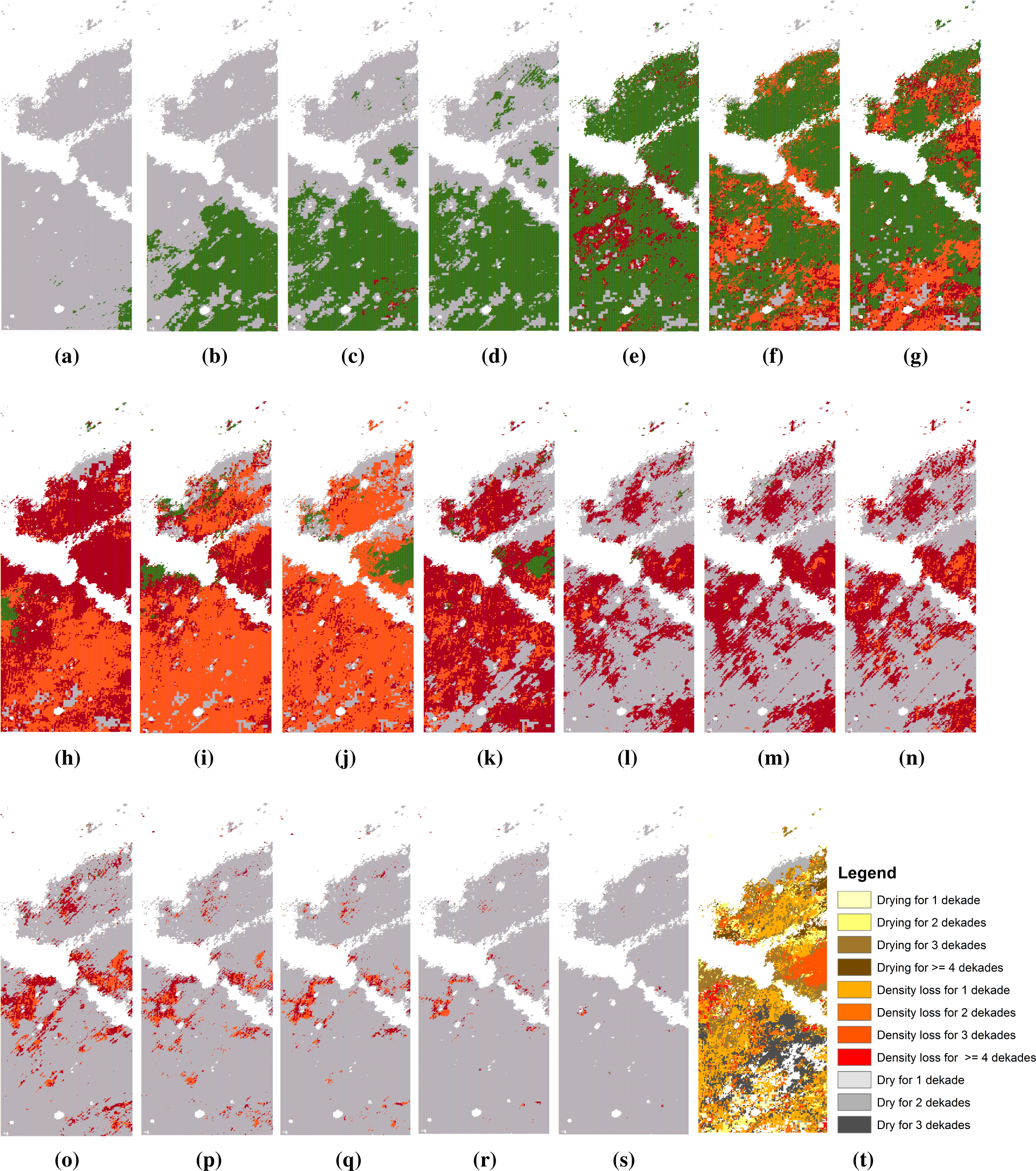

| Attribute | Possible Values |
|---|---|
| Date | 11 January 2009–20 June 2011 |
| Phenological stage | Sprout/Green/Greening/Drying/Dry |
| Total cover | Low/Moderate/Dense |
| Annual crop cover | 0%–100% |
| Perennial crop cover | 0%–100% |
| Prospected surface | 0–100,000 hectares |
| Infested surface | 0–100,000 hectares |
| Control action | Yes/No |
| Habitat | Wadi/Interdune/Plains/Basin |
| Metrics | Definition |
|---|---|
| NDVI − NDTI | difference between NDVI − NDTI |
| NDVI slope over one past 10-day interval | |
| NDTI slope over one past 10-day interval | |
| NDVI slope over two past 10-day intervals | |
| NDTI slope over two past 10-day intervals | |
| NDVI slope over the past 10-day interval to the next 10-day interval | |
| NDTI slope over the past 10-day interval to the next 10-day interval | |
| the cumulative sum of the NDVI slopes over each two past 10-day intervals | |
| the cumulative sum of the NDTI slopes over each two past 10-day intervals | |
| difference of NDVI and NDTI slope over two past 10-day intervals | |
| sum of NDVI and NDTI slope over two past 10-day intervals |
| Metrics | Raw Data | Smoothed Data | ||||||
|---|---|---|---|---|---|---|---|---|
| Growth-Decrease | Density-Drying | Growth-Decrease | Density-Drying | |||||
| AUC | OA | AUC | OA | AUC | OA | AUC | OA | |
| 88.38 | 82.70 | 59.35 | 59.09 | 93.81 | 87.78 | 52.94 | 57.96 | |
| 92.50 | 87.04 | 55.73 | 60.78 | 93.21 | 88.04 | 48.83 | 55.61 | |
| 93.11 | 87.72 | 55.63 | 60.92 | 93.87 | 88.40 | 50.26 | 55.95 | |
| 87.59 | 83.13 | 64.17 | 65.15 | 96.07 | 91.39 | 56.81 | 59.52 | |
| 70.14 | 69.84 | 69.68 | 66.16 | 73.18 | 70.77 | 71.55 | 67.67 | |
| 74.82 | 73.82 | 64.98 | 64.86 | 78.63 | 75.20 | 62.22 | 64.49 | |
| 73.48 | 72.87 | 70.71 | 66.38 | 78.43 | 73.87 | 68.12 | 66.83 | |
| 76.25 | 72.45 | 72.80 | 70.37 | 81.45 | 78.12 | 75.12 | 71.36 | |
| NDVI − NDTI | 70.32 | 64.66 | 66.99 | 51.59 | 86.18 | 80.69 | 51.20 | 51.59 |
| 85.04 | 78.44 | 52.63 | 54.33 | 91.43 | 85.12 | 54.73 | 59.13 | |
| 89.22 | 85.27 | 61.56 | 64.35 | 66.29 | 62.09 | 66.35 | 51.59 | |
| Classifiers | Omission Errors | Commission Errors | F1-score | OA | κ | ||||||
|---|---|---|---|---|---|---|---|---|---|---|---|
| Growth | Dens. | Sen. | Growth | Dens. | Sen. | Growth | Dens. | Sen. | |||
| DT | 16 | 46 | 29 | 13 | 33 | 42 | 85 | 59 | 63 | 71 | 56 |
| SVM | 14 | 49 | 25 | 15 | 30 | 41 | 85 | 58 | 65 | 72 | 57 |
| ML | 38 | 62 | 15 | 10 | 40 | 53 | 72 | 46 | 60 | 61 | 42 |
| DTSmoothing | 11 | 36 | 31 | 7 | 32 | 40 | 90 | 65 | 63 | 76 | 63 |
| SVMSmoothing | 9 | 43 | 27 | 10 | 29 | 38 | 89 | 62 | 66 | 76 | 63 |
| MLSmoothing | 31 | 51 | 13 | 5 | 27 | 54 | 79 | 57 | 59 | 67 | 51 |
© 2015 by the authors; licensee MDPI, Basel, Switzerland This article is an open access article distributed under the terms and conditions of the Creative Commons Attribution license (http://creativecommons.org/licenses/by/4.0/).
Share and Cite
Renier, C.; Waldner, F.; Jacques, D.C.; Babah Ebbe, M.A.; Cressman, K.; Defourny, P. A Dynamic Vegetation Senescence Indicator for Near-Real-Time Desert Locust Habitat Monitoring with MODIS. Remote Sens. 2015, 7, 7545-7570. https://doi.org/10.3390/rs70607545
Renier C, Waldner F, Jacques DC, Babah Ebbe MA, Cressman K, Defourny P. A Dynamic Vegetation Senescence Indicator for Near-Real-Time Desert Locust Habitat Monitoring with MODIS. Remote Sensing. 2015; 7(6):7545-7570. https://doi.org/10.3390/rs70607545
Chicago/Turabian StyleRenier, Cécile, François Waldner, Damien Christophe Jacques, Mohamed Abdallahi Babah Ebbe, Keith Cressman, and Pierre Defourny. 2015. "A Dynamic Vegetation Senescence Indicator for Near-Real-Time Desert Locust Habitat Monitoring with MODIS" Remote Sensing 7, no. 6: 7545-7570. https://doi.org/10.3390/rs70607545
APA StyleRenier, C., Waldner, F., Jacques, D. C., Babah Ebbe, M. A., Cressman, K., & Defourny, P. (2015). A Dynamic Vegetation Senescence Indicator for Near-Real-Time Desert Locust Habitat Monitoring with MODIS. Remote Sensing, 7(6), 7545-7570. https://doi.org/10.3390/rs70607545