
Snow Cover Variations and Controlling Factors at Upper Heihe River Basin, Northwestern China


Abstract
:
1. Introduction
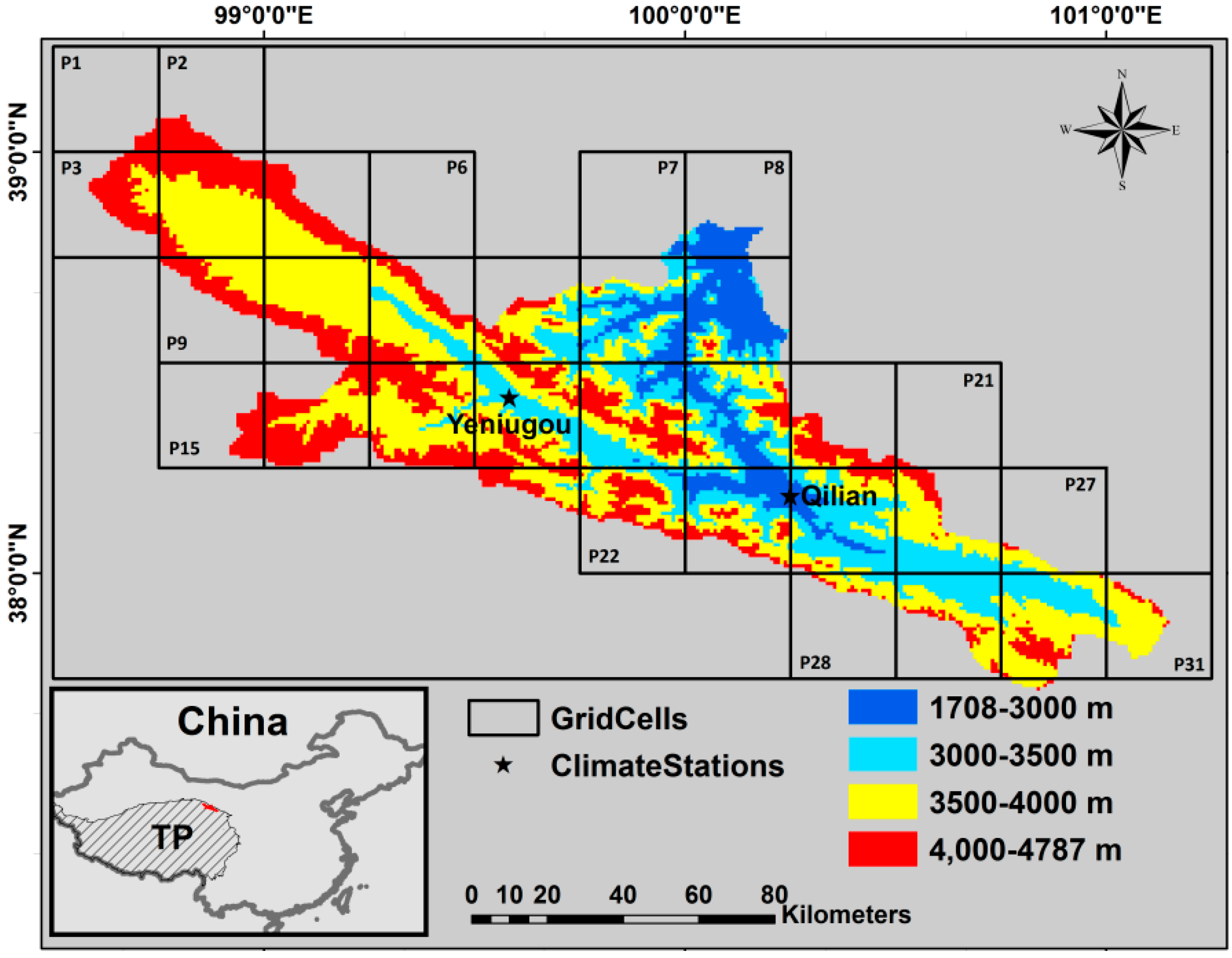
2. Study Area
3. Data and Methodology
3.1. Data
3.1.1. SRTM DEM
3.1.2. Snow Cover Data
3.1.3. Temperature
3.1.4. Precipitation Data
3.2. Methods
3.2.1. Deviation of Air Temperature from LST Data
- (i)
- MOD10A2 8-day snow products from HY2002 to HY2007 are used to separate snow and no snow periods for the two station pixels.
- (ii)
- MOD11A2 8-day LST data from HY2002 to HY2007 are extracted for the two stations and are then separated into snow and no snow periods based on the MOD10A2 snow product analysis.
- (iii)
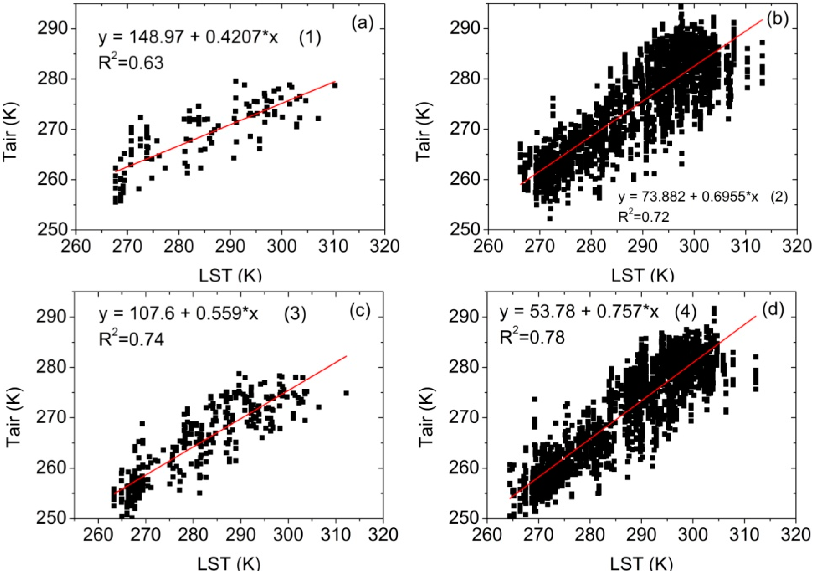
- The regression equations between 8-day mean air temperatures measured at a station and 8-day MODIS LST at the station pixel for the same period HY2002 to HY2007, for snow and no snow cases, are derived, as shown in Figure 2. These equations (unit K) are: (1) y = 148.97 + 0.4209x; (2) y = 73.882 + 0.6955x; (3) y = 107.6 + 0.559x; and (4) y = 53.78 + 0.757x. There are many more data in the no-snow case than the snow case for both stations, with R2 values of the no-snow case larger than those of the snow case. The R2 values at Yeniugou station are larger than R2 values at Qilian station. This might indicate that the Tair is correlated better with LST in higher altitude (Yeniugou station) than at lower altitude (Qilian station). The difference of land-surface and air temperatures dependence is related to the aerodynamic resistance to heat transfer [36,37]. At higher altitude, the air temperature is lower. Therefore the heat transfer is also lower, resulting in smaller differences between air temperature and land-surface temperature. This might be the reason that the correlation coefficient between air temperature and LST is higher at higher altitude than that at lower altitude.
- (iv)
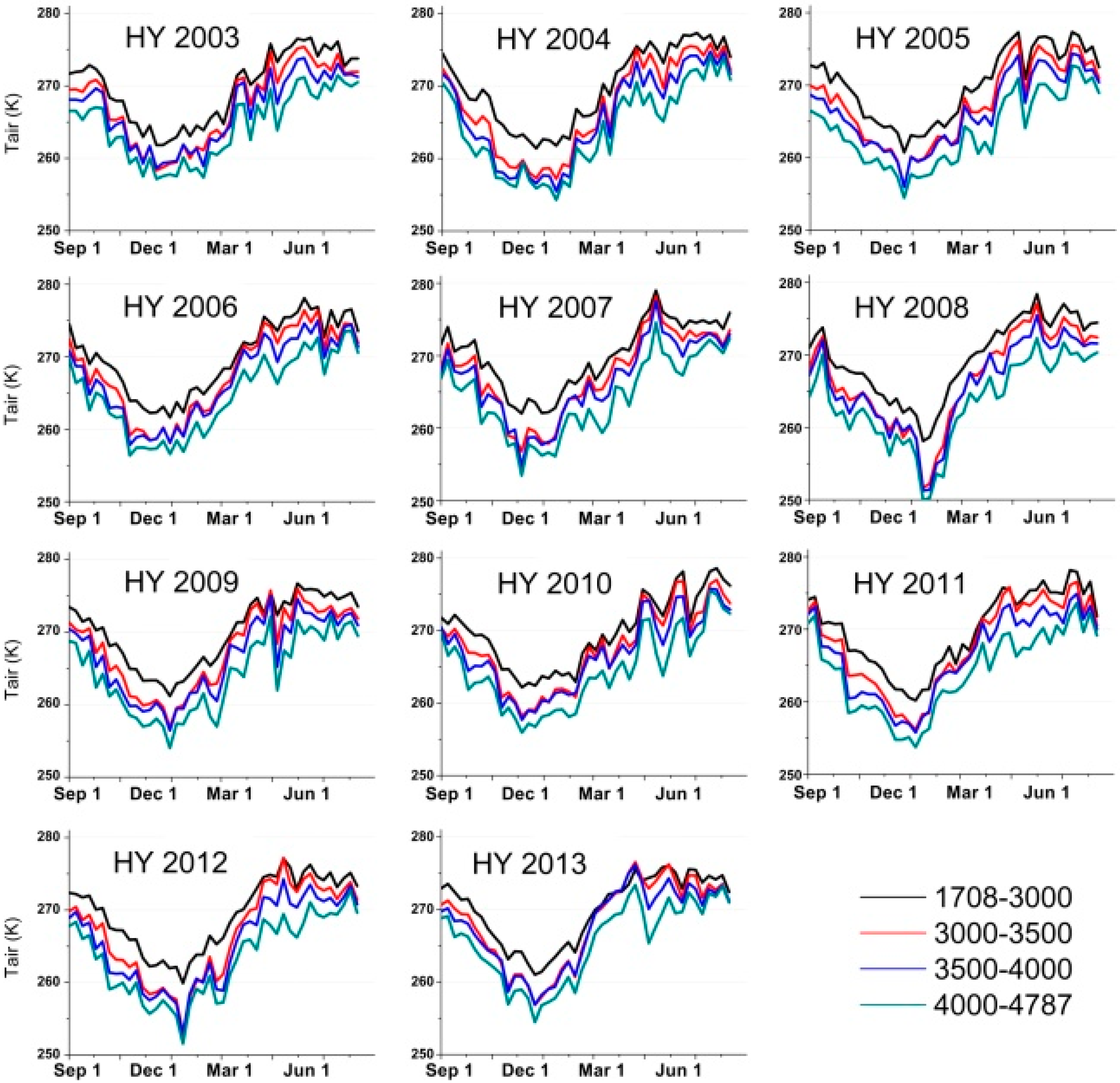
- Simulate Tair of each cell based on the MODIS LST, using the above equations in Figure 2. The Equations (1) and (2) (snow and no snow cases) derived at the Qilian station (2787 m) are used to simulate Tair in the elevation zone (a) 1708–3000 m. Equations (3) and (4) (snow and no snow cases) derived at the Yeniugou station (3320 m) are used to simulate Tair for elevation zones (b) 3000–3500 m; (c) 3500–4000 m; and (d) 4000–4787 m. Using the equations derived from the Yeniugou station (in Zone b) for the zones (c) and (d) might cause some errors; however, the difference should be minor and should not impact the overall patterns of Tair change.
3.2.2. Gridding Partition
3.2.3. Snow Cover Mapping Methods
3.2.4. Correlation between Climate Factors and Snow Cover Area (SCA)
4. Results
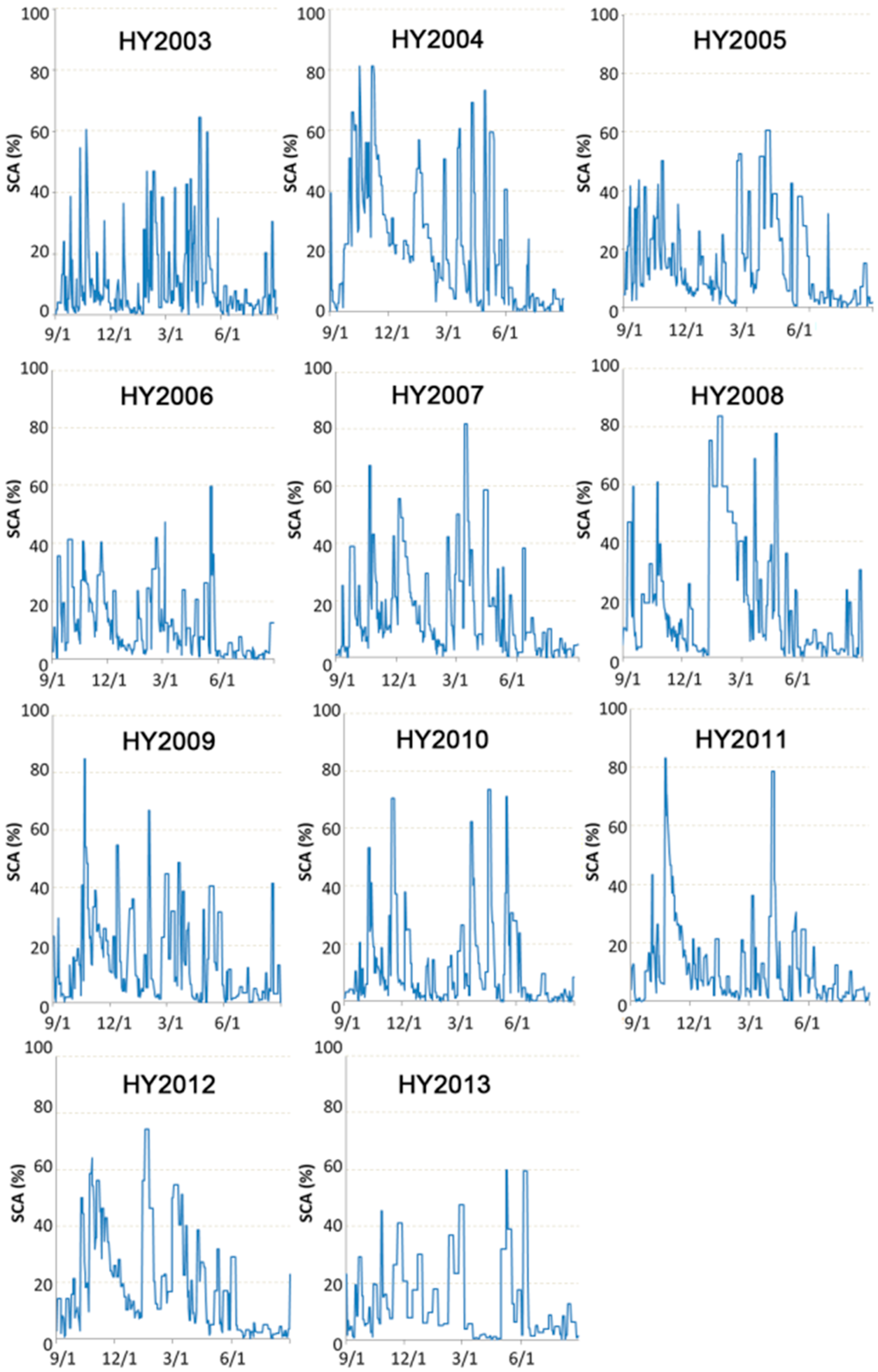
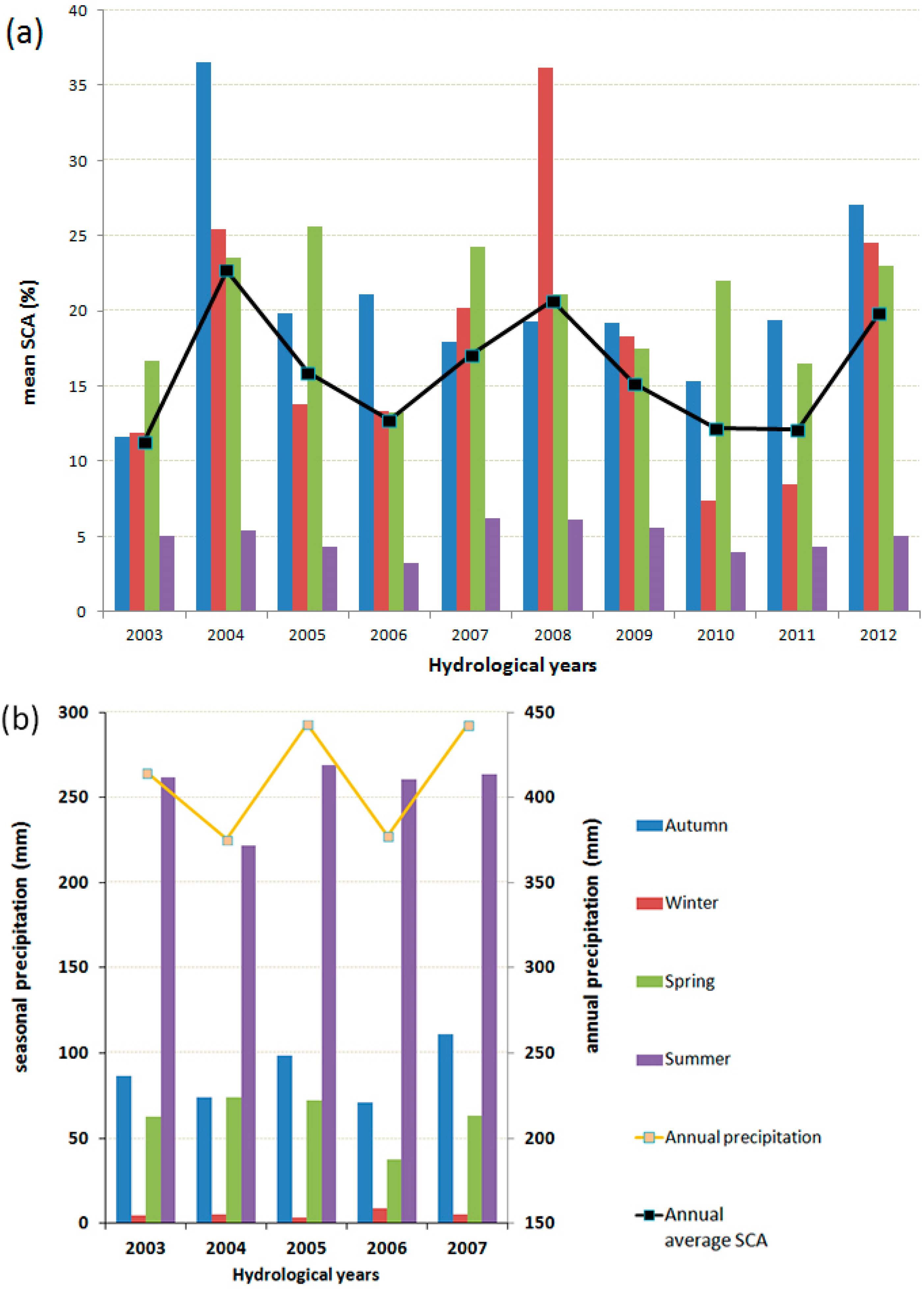
4.1. Characteristics of Temporal Variations of Snow Cover Areas (SCA)

| Hydrological Year | Number of Peaks | |||
|---|---|---|---|---|
| Autumn | Winter | Spring | Summer | |
| 2003 | 2 (55%, 60%) | 3 (45%, 45%, 40%) | 5 (40%, 40%, 40%, 65%, 60%) | 0 |
| 2004 | 6 (40%, 50%, 60%, 80%, 55%, 80%) | 2 (55%, 50%) | 5 (75%, 70%, 60%, 60%, 40%) | 0 |
| 2005 | 5 (40%, 40%, 40%, 40%, 50%) | 1 (50%) | 4 (40%, 50%, 60%, 40%) | 0 |
| 2006 | 3 (40%, 40%, 40%) | 1 (40%) | 2 (50%, 60%) | 0 |
| 2007 | 4 (40%, 70%, 40%, 40%) | 2 (55%, 40%) | 3 (50%, 80%, 60%) | 0 |
| 2008 | 4 (50%, 60%, 60%, 40%) | 2 (75%, 85%) | 5 (40%, 40%, 70%, 40%, 80%) | 0 |
| 2009 | 4 (40%, 85%, 40%) | 2 (55%, 65%) | 3 (45%, 50%, 40%) | 1 (40%) |
| 2010 | 3 (50%, 40%, 70%) | 0 | 3 (60%, 70%, 70%) | 0 |
| 2011 | 2 (45%, 85%) | 0 | 1 (80%) | 0 |
| 2012 | 5 (50%, 60%, 55%, 45%, 40%) | 1 (75%) | 3 (55%, 50%, 40%) | 0 |
| 2013 | 2 (40%, 40%) | 1 (40%) | 2 (60%, 60%) | 0 |

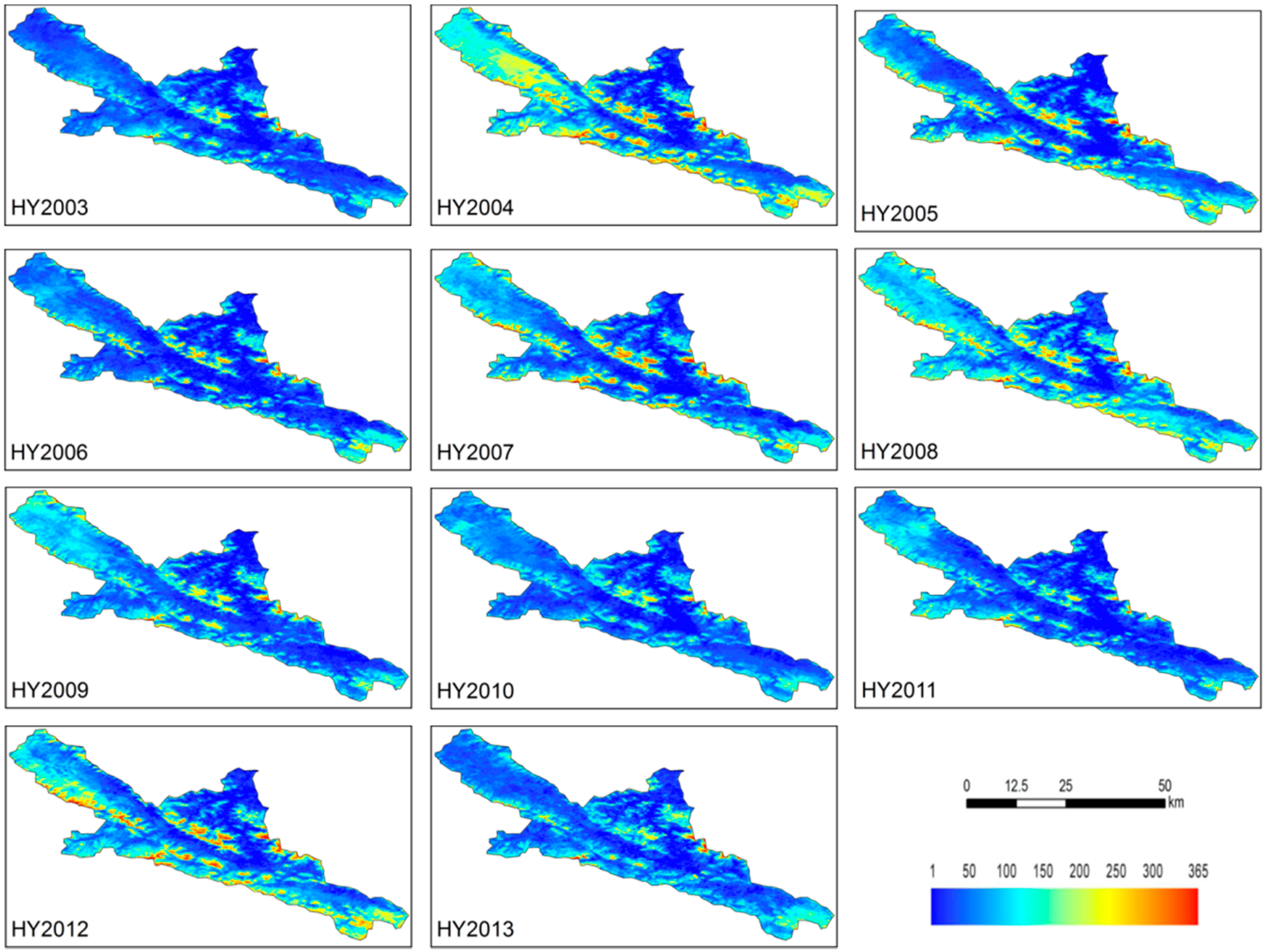
4.2. Characteristics of Spatial and Temporal Variations of Snow Cover Days (SCD)

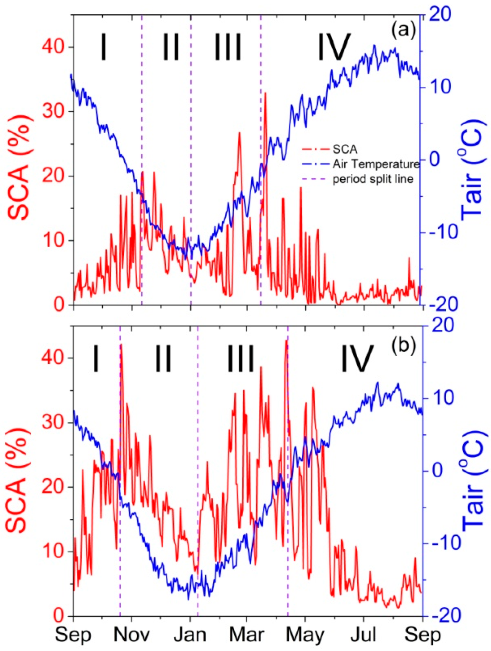
4.3. Correlation between Air Temperature and Snow Cover


| Snow Period | I | II | III | IV |
|---|---|---|---|---|
| Qilian | −0.72 | 0.77 | 0.54 | −0.74 |
| Yeniugou | −0.70 | 0.62 | 0.38 | −0.52 |
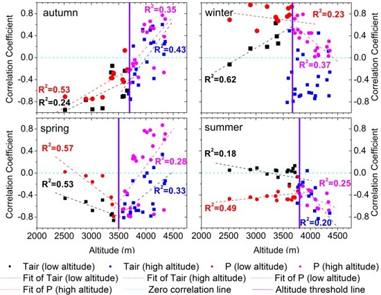
4.4. Seasonal and Altitude Effects on Correlations between Snow Cover and Climate Factors

5. Discussion
5.1. Altitude Factor
5.2. Seasonal Factor
5.3. Sublimation Factor
| Month | Sublimation (mm) | Precipitation (mm) | Ratio (S/P) |
|---|---|---|---|
| January | 59.9 | 31.6 | 1.90 |
| February | 52.7 | 32.0 | 1.65 |
| March | 24.5 | 34.1 | 0.72 |
| 1 April–12 May | 3.7 | 106.9 | 0.03 |
5.4. Regional Factor
6. Conclusions
Acknowledgments
Author Contributions
Conflicts of Interest
References
- Groisman, P.Y.; Karl, T.R.; Knight, R.W.; Stenchikov, G.L. Changes of snow cover, temperature, and radiative heat balance over the Northern Hemisphere. J. Clim. 1994, 7, 1633–1656. [Google Scholar] [CrossRef]
- Robinson, D.A.; Dewey, K.F.; Heim, R.R., Jr. Global snow cover monitoring: An update. Bull. Amer. Meteor. Soc. 1993, 74, 1689–1696. [Google Scholar] [CrossRef]
- Qin, D.; Liu, S.; Li, P. Snow cover distribution, variability, and response to climate change in Western China. J. Clim. 2006, 19, 1820–1833. [Google Scholar]
- Shang, Z.H.; Gibb, M.J.; Long, R.J. Effect of snow disasters on livestock farming in some rangeland regions of China and mitigation strategies—A review. Rangel. J. 2012, 34, 89–101. [Google Scholar] [CrossRef]
- Wang, W.; Liang, T.; Huang, X.; Feng, Q.; Xie, H.; Liu, X.; Chen, M.; Wang, X. Early warning of snow-caused disasters in pastoral areas on Tibetan Plateau. Nat. Hazards Earth Syst. 2013, 13, 1411–1425. [Google Scholar] [CrossRef]
- Mijinyawa, Y.; Dlamini, S.S. Impact assessment of water scarcity at Somntongo in the lowveld region of Swaziland. Sci. Res. Essays. 2008, 3, 061–065. [Google Scholar]
- Painter, T.H.; Rittger, K.; McKenzie, C.; Slaughter, P.; Davis, R.E.; Dozier, J. Retrieval of subpixel snow covered area, grain size, and albedo from MODIS. Remote Sens. Environ. 2009, 113, 868–879. [Google Scholar] [CrossRef]
- Barnett, T.P.; Adam, J.C.; Lettenmaier, D.P. Potential impacts of a warming climate on water availability in snow-dominated regions. Nature 2005, 438, 303–309. [Google Scholar] [CrossRef] [PubMed]
- Viviroli, D.; Dürr, H.H.; Messerli, B.; Meybeck, M.; Weingartner, R. Mountains of the world, water towers for humanity: Typology, mapping, and global significance. Water Resour. Res. 2007, 43. [Google Scholar] [CrossRef]
- Zhao, Y.; Nan, Z.; Chen, H.; Li, X.; Jayakumar, R.; Yu, W. Integrated hydrologic modeling in the inland (HRB), Northwest China. Sci. Cold Arid Reg. 2013, 5, 0035–0050. [Google Scholar]
- Cheng, G.D.; Li, X.; Zhao, W.Z.; Xu, Z.M.; Feng, Q.; Xiao, S.C.; Xiao, H.L. Integrated study of the water-ecosystem-economy in the (HRB). Natl. Sci. Rev. 2014, 1, 413–428. [Google Scholar] [CrossRef]
- Ge, Y.; Li, X.; Huang, C.; Nan, Z. A Decision Support System for irrigation water allocation along the middle reaches of the (HRB), Northwest China. Environ. Modell. Softw. 2013, 47, 182–192. [Google Scholar] [CrossRef]
- Li, X.; Cheng, G.; Liu, S.; Xiao, Q.; Ma, M.; Jin, R.; Che, T.; Liu, Q.; Wang, W.; Qi, Y.; et al. Heihe watershed allied telemetry experimental research (hiwater): Scientific objectives and experimental design. Bull. Amer. Meteor. Soc. 2013, 94, 1145–1160. [Google Scholar] [CrossRef]
- Jin, R.; Li, X.; Yan, B.P.; Li, X.H.; Luo, W.M.; Ma, M.G.; Guo, J.W.; Kang, J.; Zhu, Z.L.; Shao, S.J. A nested eco-hydrological wireless sensor network for capturing the surface heterogeneity in the midstream area of the (HRB), China. IEEE Geosci. Remote Sens. Lett. 2014, 11, 2015–2019. [Google Scholar] [CrossRef]
- Dai, L.; Che, T. Spatiotemporal variability in snow cover from 1987 to 2011 in northern China. J. Appl. Remote Sens. 2013, 8. [Google Scholar] [CrossRef]
- Hall, D.K.; Riggs, G.A. Accuracy assessment of the MODIS snowcover products. Hydrol. Process. 2007, 21, 1534–1547. [Google Scholar] [CrossRef]
- Maurer, E.P.; Rhoads, J.D.; Dubayah, R.O.; Lettenmaier, D.P. Evaluation of the snow covered area data product from MODIS. Hydrol. Process. 2003, 17, 59–71. [Google Scholar] [CrossRef]
- Parajka, J.; Blöschl, G. Validation of MODIS snow cover images over Austria. Hydrol. Earth Syst. Sci. 2006, 10, 679–689. [Google Scholar] [CrossRef]
- Xie, H.; Wang, X.; Liang, T. Development and assessment of combined Terra and Aqua snow cover products in Colorado Plateau, USA and northern Xinjiang, China. J. Appl. Remote Sens. 2009, 3. [Google Scholar] [CrossRef]
- Gao, Y.; Xie, H.; Yao, T.; Xue, C. Integrated assessment on multi-temporal and multi-sensor combination for reducing cloud obscuration of MODIS snow cover products at the Pacific Northwestern USA. Remote Sens. Environ. 2010, 114, 1662–1675. [Google Scholar] [CrossRef]
- Zhang, G.; Xie, H.; Yao, T.; Liang, T.; Kang, S. Snow cover dynamics of four lake basins over Tibetan Plateau using time series MODIS data (2001–2010). Water Resour. Res. 2012, 48. [Google Scholar] [CrossRef]
- Chen, S.; Yang, Q.; Xie, H.; Zhang, H.; Lu, P.; Zhou, C. Spatio-temporal dynamics of snow cover in Northeast China based on flexible multiday combinations of MODIS snow cover products. J. Appl. Remote Sens. 2014, 8, 084685. [Google Scholar] [CrossRef]
- Li, H.; Tang, Z.; Wang, J.; Che, T.; Pan, X.; Huang, C.; Wang, X. Synthesis method for simulating snow distribution utilizing remotely sensed data for the Tibetan Plateau. J. Appl. Remote Sens. 2014, 8. [Google Scholar] [CrossRef]
- Morán-Tejeda, E.; López-Moreno, J.I.; Beniston, M. The changing roles of temperature and precipitation on snowpack variability in Switzerland as a function of altitude. Geophys. Res. Lett. 2013, 40, 2131–2136. [Google Scholar] [CrossRef]
- Beniston, M. Is snow in the Alps receding or disappearing? WIREs Clim. Change 2012, 3, 349–358. [Google Scholar] [CrossRef]
- Laternser, M.; Schneebeli, M. Long-term snow climate trends of the Swiss Alps (1931–1999). Int. J. Climatol. 2003, 23, 733–750. [Google Scholar] [CrossRef]
- Marty, C. Regime shift of snow days in Switzerland. Geophys. Res. Lett. 2008, 35. [Google Scholar] [CrossRef]
- Scherrer, S.C.; Appenzeller, C.; Laternser, M. Trends in Swiss Alpine snow days: The role of local- and large-scale climate variability. Geophys. Res. Lett. 2004, 31. [Google Scholar] [CrossRef]
- Wang, J.; Li, H.; Hao, X. Responses of snowmelt runoff to climatic change in an inland river basin, Northwestern China, over the past 50 years. Hydrol. Earth Sys. Sci. 2010, 14, 1979–1987. [Google Scholar] [CrossRef]
- Li, X.; Li, X.; Li, Z.; Ma, M.; Wang, J.; Xiao, Q.; Liu, Q.; Che, T.; Chen, E.; Yan, G.; et al. Watershed allied telemetry experimental research. J. Geophys. Res.: Atmos. 2009, 114. [Google Scholar] [CrossRef]
- Wan, Z.; Zhang, Y.; Zhang, Q.; Li, Z. Quality assessment and validation of the modis global land surface temperature. Int. J. Remote Sens. 2004, 25, 261–274. [Google Scholar] [CrossRef]
- Yu, W.; Ma, M.; Wang, X.; Song, Y.; Tan, J. Validation of MODIS land surface temperature products using ground measurements in the Heihe River Basin. Proc. SPIE 2011, 8174, 817421–817431. [Google Scholar]
- National Center for Atmospheric Research Staff (NCAR). The Climate Data Guide: APHRODITE: Asian Precipitation—Highly-Resolved Observational Data Integration towards Evaluation of Water Resources; National Center for Atmospheric Research Staff (NCAR): Boulder, CO, USA, 2014. [Google Scholar]
- Yatagai, A.; Kamiguchi, K.; Arakawa, O.; Hamada, A.; Yasutomi, N.; Kitoh, A. APHRODITE: Constructing a long-term daily gridded precipitation dataset for asia based on a dense network of rain gauges. Bull. Amer. Meteor. Soc. 2012, 93, 1401–1415. [Google Scholar] [CrossRef]
- Gallo, K.; Hale, R.; Tarpley, D.; Yu, Y. Evaluation of the relationship between air and land Surface Temperature under clear- and cloudy-sky conditions. J. Appl. Meteor. Climatol. 2011, 50, 767–775. [Google Scholar] [CrossRef]
- Urban, M.; Eberle, J.; Hüttich, C.; Schmullius, C.; Herold, M. Comparison of satellite-derived land surface temperature and air temperature from meteorological stations on the pan-Arctic Scale. Remote Sens. 2013, 5, 2348–2367. [Google Scholar] [CrossRef]
- Shamir, E.; Georgakakos, K.P. MODIS Land surface temperature as an index of surface air temperature for operational snowpack estimation. Rem. Sens. Environ. 2014, 152, 83–98. [Google Scholar] [CrossRef]
- Liang, T.; Huang, X.; Wu, C.; Liu, X.; Li, W.; Guo, Z.; Ren, J. Application of MODIS data on snow cover monitoring in pastoral area: A case study in the Northern Xinjiang, China. Rem. Sens. Environ. 2008, 112, 1514–1526. [Google Scholar] [CrossRef]
- King, M.D.; Kaufman, Y.J.; Menzel, W.P.; Tanre, D. Remote sensing of cloud, aerosol, and water vapor properties from the Moderate Resolution Imaging Spectrometer (MODIS). IEEE Trans. Geosci. Rem. Sens. 1992, 30, 2–27. [Google Scholar] [CrossRef]
- Wang, X.; Xie, H. New methods for studying the spatiotemporal variation of snow cover based on combination products of MOIDS Terra and Aqua. J. Hydrol. 2009, 371, 192–200. [Google Scholar] [CrossRef]
- Liston, G.E.; Sturm, M. A snow-transport model for complex terrian. J. Glaciol. 1998, 44, 498–516. [Google Scholar]
- Pomeroy, J.W.; Gray, D.M.; Shook, K.R.; Toth, B.; Essery, R.L.H.; Pietroniro, A.; Hedstrom, N. An evaluation of snow accumulation and ablation processes for land surface modelling. Hydrol. Process. 1998, 12, 2339–2367. [Google Scholar] [CrossRef]
- Beniston, M.; Keller, F.; Goyette, S. Snow pack in the SwissAlps under changing climatic conditions: An empirical approach forclimate impacts studies. Theor. Appl. Climatol. 2003, 74, 19–31. [Google Scholar] [CrossRef]
- Marty, C.; Blanchet, J. Long-term changes in annual maximum snow depth and snow fall in Switzerland based on extreme value statistics. Clim. Chang. 2011, 111, 705–721. [Google Scholar] [CrossRef]
- Zhang, Y.; Suzuki, K.; Kadota, T.; Ohata, T. Sublimation from snow surface in southern mountain taiga of eastern Siberia. J. Geophys. Res. 2004, 109. [Google Scholar] [CrossRef]
- Hood, E.; Williams, M.; Cline, D. Sublimation from a seasonal snowpack at a continental, mid-latitude alpine site. Hydrol. Process. 1999, 13, 1781–1797. [Google Scholar] [CrossRef]
- Jackson, S.I.; Prowse, T.D. Spatial variation of snowmelt and sublimation in a high-elevation semi-desert basin of western Canada. Hydrol. Process. 2009, 23, 2611–2627. [Google Scholar] [CrossRef]
- Fassnacht, S.R. Estimating Alter-shielded gauge snow fall undercatch, snowpack sublimation, and blowing snow transport at six sites in the coterminous USA. Hydrol. Process. 2004, 18, 3481–3492. [Google Scholar] [CrossRef]
- Tarboton, D.G. Measurements and Modeling of Snow Energy Balance and Sublimation from Snow. Available online: http://digitalcommons.usu.edu/water_rep/61 (accessed on 15 May 2015).
- Li, H.Y.; Wang, J.; Hao, X.H. Role of blowing snow in snow processes in Qilian Mountainous region. Sci. Cold Arid Reg. 2014, 6, 0124–0130. [Google Scholar]
- Li, H.; Wang, J.; Bai, Y.; Li, Z.; Dou, Y. The snow hydrological processes during a Representative snow cover period in Binggou Watershed in the upper reaches of Heihe River. J. Glaciol. Geocryol. 2009, 31, 294–300. [Google Scholar]
- Li, Z.; Deng, X.; Wu, F.; Hasan, S.S. Scenario analysis for water resources in response to land use change in the middle and upper reaches of the Heihe River Basin. Sustainability 2015, 7, 3086–3108. [Google Scholar]
- Schulz, O.; de Jong, C. Snowmelt and sublimation: Field experiments and modelling in the High Atlas Mountains of Morocco. Hydrol. Earth Syst. Sci. 2004, 8, 1076–1089. [Google Scholar] [CrossRef]
- Cheng, J.J.; Jiang, F.Q.; Xue, C.X.; Xin, G.W.; Li, K.C.; Yang, Y.H. Characteristics of the disastrous wind-sand environment along railways in the Gobi area of Xinjiang, China. Atmos. Environ. 2015, 102, 344–354. [Google Scholar] [CrossRef]
- Zhang, K.; Qu, J.; Han, Q.; An, Z. Wind energy environments and Aeolian sand characteristics along the Qinghai–Tibet Railway, China. Sediment. Geol. 2012, 273, 91–96. [Google Scholar] [CrossRef]
© 2015 by the authors; licensee MDPI, Basel, Switzerland. This article is an open access article distributed under the terms and conditions of the Creative Commons Attribution license (http://creativecommons.org/licenses/by/4.0/).
Share and Cite
Bi, Y.; Xie, H.; Huang, C.; Ke, C. Snow Cover Variations and Controlling Factors at Upper Heihe River Basin, Northwestern China. Remote Sens. 2015, 7, 6741-6762. https://doi.org/10.3390/rs70606741
Bi Y, Xie H, Huang C, Ke C. Snow Cover Variations and Controlling Factors at Upper Heihe River Basin, Northwestern China. Remote Sensing. 2015; 7(6):6741-6762. https://doi.org/10.3390/rs70606741
Chicago/Turabian StyleBi, Yunbo, Hongjie Xie, Chunlin Huang, and Changqing Ke. 2015. "Snow Cover Variations and Controlling Factors at Upper Heihe River Basin, Northwestern China" Remote Sensing 7, no. 6: 6741-6762. https://doi.org/10.3390/rs70606741
APA StyleBi, Y., Xie, H., Huang, C., & Ke, C. (2015). Snow Cover Variations and Controlling Factors at Upper Heihe River Basin, Northwestern China. Remote Sensing, 7(6), 6741-6762. https://doi.org/10.3390/rs70606741