An Improved Endmember Selection Method Based on Vector Length for MODIS Reflectance Channels

Abstract

Endmember selection is the basis for sub-pixel land cover classifications using multiple endmember spectral mixture analysis (MESMA) that adopts variant endmember matrices for each pixel to mitigate errors caused by endmember variability in SMA. A spectral library covering a large number of endmembers can account for endmember variability, but it also lowers the computational efficiency. Therefore, an efficient endmember selection scheme to optimize the library is crucial to implement MESMA. In this study, we present an endmember selection method based on vector length. The spectra of a land cover class were divided into subsets using vector length intervals of the spectra, and the representative endmembers were derived from these subsets. Compared with the available endmember average RMSE (EAR) method, our approach improved the computational efficiency in endmember selection. The method accuracy was further evaluated using spectral libraries derived from the ground reference polygon and Moderate Resolution Imaging Spectroradiometer (MODIS) imagery respectively. Results using the different spectral libraries indicated that MESMA combined with the new approach performed slightly better than EAR method, with Kappa coefficient improved from 0.75 to 0.78. A MODIS image was used to test the mapping fraction, and the representative spectra based on vector length successfully modeled more than 90% spectra of the MODIS pixels by 2-endmember models.

1. Introduction

The accuracy of sub-pixel classification of land cover types using spectral mixture analysis (SMA) or multiple endmember spectral mixture analysis (MESMA) is strongly affected by the selection of pure spectra, or endmembers [1,2,3]. MESMA based on SMA commonly uses variant endmembers for image pixels, and the appropriate endmember model is usually determined for a pixel via the metric of minimum root mean squared error (RMSE) of model fits and other constrained conditions [2]. In order to sufficiently model the complex land cover types using MESMA, an endmember library of an enormous number of spectra needs to be established from reference spectra or image pure pixels to explain the spectral variability. A large number of spectra cause a heavy computational burden and a complicated interpretation of model results [3,4]. Therefore, endmember selection optimizing representative spectra from the endmember library is a crucial component for MESMA, as it balances the accuracy of modeled fractions and the computational efficiency of model fits [3,5].

Endmember selection methods for MESMA were elaborated in previous studies. A count-based (CoB) method focused on the number of successful model fit within a library, and representative endmembers for each land cover class were chose with the spectra that successfully modeled the greatest number starting from all spectra to the spectra of a class remained unmodeled [2,6]. Another method, the minimum endmember average RMSE (EAR), based on the average error of a spectrum modeling all spectra of a class which was determined by MESMA, and the representative endmember is the minimum EAR spectrum within a class [3]. Similar to minimum EAR, the minimum average spectral angle (MASA) used spectral angle to select the representative spectra, and the comparison between spectral angle mapping (SAM) and MESMA indicates that SMA is more sensitive for selection of lower albedo spectra [7]. An iterative endmember selection (IES) focused on the classification accuracy of endmembers for the endmember library with all classes, which selected the spectra with the higher kappa coefficient of classification [8]. The above methods have been used for MESMA to successfully map land cover classes [9,10,11]. A combined method, hybrid IES-CoB/EAR selection, was also developed to select endmembers for mapping plant, which synthesized the two previous approaches and successfully modeled plant species [5].

For these approaches, two steps were involved: (1) a spectral matching algorithm was used for model fits or similarity measures (e.g., SMA, MESMA, SAM); (2) a quantitative metric was used to select a set of endmembers (e.g., the minimizing RMSE, the minimizing spectral angle, maximizing kappa). For example, SMA was applied to iteratively fitting each endmember to other spectra within a library, and the representative endmembers were selected with the spectra meeting the criteria RMSE of SMA. Iterative model fits of SMA to all endmember pairs would hamper the selection efficiency if a large number of spectra were used. Meanwhile, some quantitative metrics may miss endmembers that represent a class, when endmember classes are highly variable. For example, the minimum EAR poorly selected representative endmembers from a highly variable class [3], and the IES method missed representative endmembers from a rare class [5].

Is it possible to choose a new quantitative metric for selection of representative spectra without iterative model fits, and widely represent a class with higher variability? Vector length of a spectrum is an important feature to construct classifier [12]. Unlike the previous quantitative metrics relying on iterative model fits, vector length could subset spectra alone without matching algorithm. MESMA is sensitive to the vector length of a modeled spectrum due to the higher correlation between the albedo and the vector length of a spectrum [7,13]. Therefore, the vector length of spectra may be a quantitative metric to divide subsets for a more variable class, and representative endmembers will be calculated by the median or average spectrum of each subset.

Due to advantages for mapping global land cover types as an optical sensor, the band channels of MODIS reflectance are highlighted in this study. The objective of this paper is to present a new method for efficiently dividing spectral subsets of endmember classes and obtaining representative endmembers based on vector length of spectra for MODIS reflectance channels.

In this paper, we test a new quantitative metric, vector length, for endmember selection. Spectra derived from reference polygon were used to compare the new method to EAR/CoB method, and a MODIS image was used to test the performance of MESMA for mapping. The next section presents the new method based on vector length and two data sets including a spectral library for comparison and a set of images (MODIS and ETM images) for mapping. The third section presents the study results. Discussions and conclusions are provided in the last two sections.

2. Methods and Data

2.1. Study Areas

Two areas were used for this study, which derived different data sets for two experiments purposes. For comparison purpose of endmember selection, we downloaded an existing data set including an original spectral library (OSL), a representative spectral library based on EAR/CoB (RSLEC), Airborne Visible Infrared Imaging Spectrometry (AVIRIS) imagery and ground reference polygons [14]. 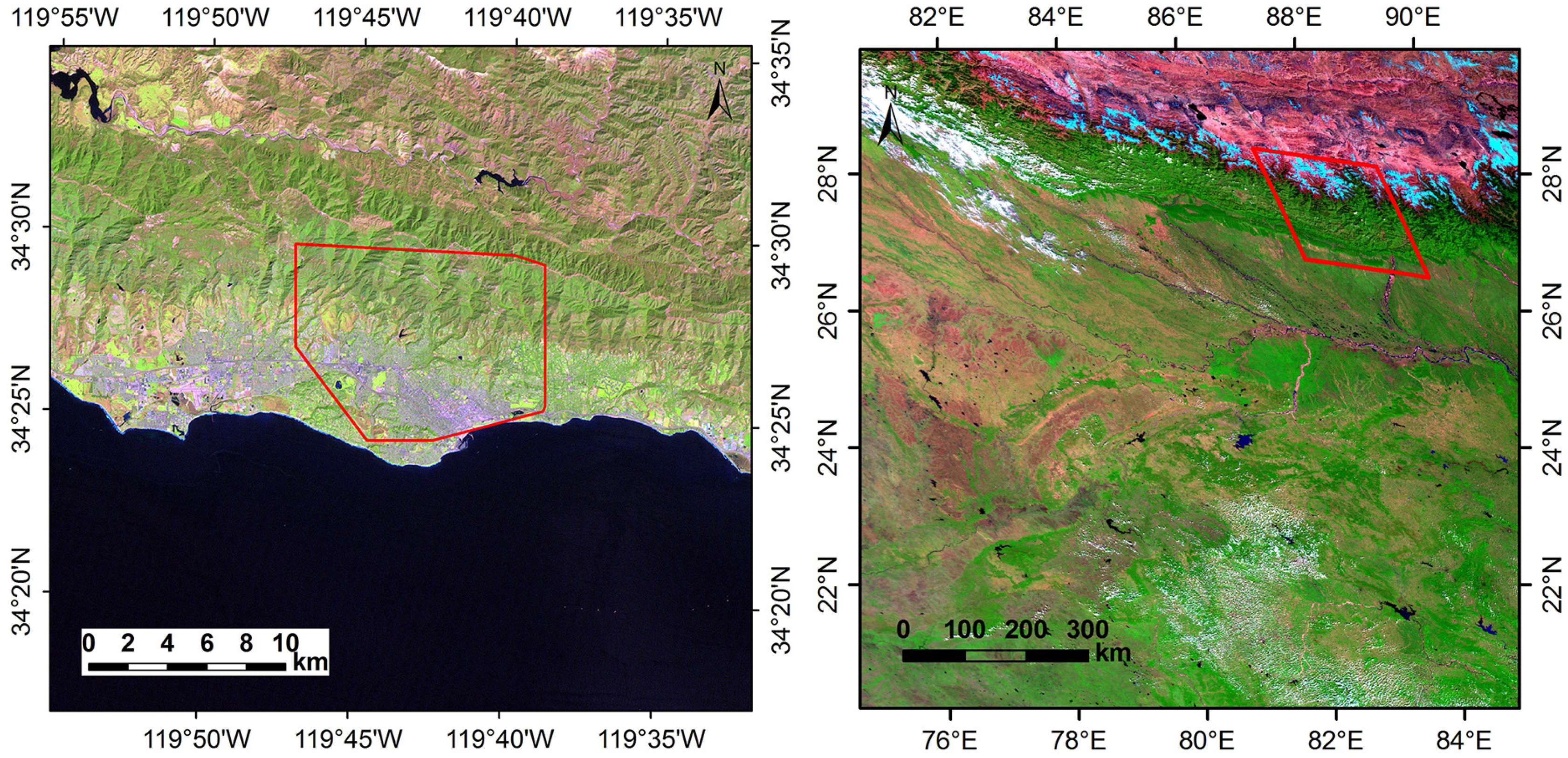The two libraries were extracted from the AVIRIS imagery over the Santa Barbara where the land cover types are dominated by vegetation, soil and urban (Figure 1a). In order to test the mapping performance using the new endmember selection, a set of imageries were processed for mapping and assessing land cover classes. The data consisted of Moderate Resolution Imaging Spectroradiometer (MODIS) and Enhanced Thematic Mapper (ETM) images (Figure 1b). To test the mapping performance of endmember selection, a set of imageries were processed for land cover map and validation, which consisted of Moderate Resolution Imaging Spectroradiometer (MODIS) and Enhanced Thematic Mapper (ETM) images (Figure 1b). Snow is a typical land cover type, and MODIS is a popular sensor for global snow mapping due to its moderate spatial resolution, higher temporal resolution and appropriate channels for detecting snow. So imageries located in the Himalayas were used to map four land cover classes that were identifiable by broad band sensors.

Figure 1. Study areas: (a) A red polygon of left image is the cover region of Airborne Visible Infrared Imaging Spectrometry (AVIRIS) in St. Babara shown as a UTM projection; (b) The right image is a scene of Moderate Resolution Imaging Spectroradiometer (MODIS) image with grid number h25v06 shown as a Sinusoidal projection, and a red parallelogram is the overlapped region between MODIS and Enhanced Thematic Mapper (ETM).

Figure 1. Study areas: (a) A red polygon of left image is the cover region of Airborne Visible Infrared Imaging Spectrometry (AVIRIS) in St. Babara shown as a UTM projection; (b) The right image is a scene of Moderate Resolution Imaging Spectroradiometer (MODIS) image with grid number h25v06 shown as a Sinusoidal projection, and a red parallelogram is the overlapped region between MODIS and Enhanced Thematic Mapper (ETM).

2.2. Data Set for Comparison

OSL was extracted from AVIRIS imagery over the Santa Barbara in 14 June 2001 using the training reference polygons, and RSLEC was selected from OSL using EAR/CoB method by “Vipertools” team [14]. Ground reference polygons were created using field land cover classes and 1-m resolution digital orthophoto quads (DOQs) [3]. OSL and RSLEC consist of 1588 and 78 spectra with five classes, respectively (Table 1). For our experiments of MODIS reflectance channels, we spectrally convolved OSL, RSLEC, and AVIRIS imagery using MODIS filter functions.

Then we constructed a library with 70 representative spectra from OSL using the new method implemented by our routine, which was named representative spectral library based on vector length (RSLVL). Each spectrum of RSLVL was the median spectrum of a subset of a land cover class, and the subset partition was mainly implemented by equal intervals of vector length for each class.

Two representative spectral libraries, RSLEC and RSLVL, based on different endmember selection methods were used to classify land over classes of the AVIRIS imagery (with MODIS reflectance channels) using 2-endmember MESMA implemented in the ENVI add-on “ViperTools” [14]. We used 2-endmember MESMA (endmember+shade) since it was simple and adequate for the comparison between two libraries. RSLVL was used as an input file for of ViperTool. The minimum and maximum fractions for software were −0.05 and 1.05 respectively, and the photometric shade was used in “ViperTools”. The accuracy of the two representative libraries was assessed by the confusion matrix comparing to pixels of true land cover classes, which were 1670 pixels extracted from the AVIRIS image using the assessing reference polygons.

2.3. Image Data for Mapping

A pair of images, MODIS and ETM, was used to test the mapping performance of MESMA using the new method. The study area overlapped between two images is located in the Himalayas (Figure 1b), and both images were acquired on 3 October 2000. The grid of MOD09GA, MODIS/Terra surface reflectance daily product, was h25v06, and the ETM was p140r041. Complex mountainous terrain with heterogeneity generally causes higher spectra variability, and it is ideal to evaluate the ability of the new method for mapping land cover classes. Four land cover classes are identifiable by MODIS and ETM using image classification techniques, which are green vegetation (GV), soil/NPV (non-photosynthetic vegetation), snow and shade/water classes. Related to the five classes in Table 1, shrub and tree are subclasses of the GV; litter and soil are subclasses of the soil/NPV. Urban is a most complicated surface class, and its spectrum is similar to soil/NPV in MODIS reflectance channels. The four land cover types can be clearly divided and identifiable by MODIS and ETM using the image classification techniques. Therefore, four classes are appropriate for fraction map within 500-m resolution of MODIS, and the fractions of MODIS pixels for the four land cover classes are mapped using MESMA and the endmember selection based on vector length.

MODIS/Terra is descending observation at local time 10:30 [15], and a higher resolution ETM image with the similar passing time was used to calculate the “true” fractions within the MODIS 500-m resolution pixel for each of the four land cover classes. The true fractions of the four classes were derived in the two main steps: classification of ETM and fraction calculation within 500-m using the classification map.

First, ETM imagery with 30-m pixels was classified with GV, soil/NPV, snow and shade/water. (1) Snow pixels of ETM were identified using SNOWMAP algorithm based on normalized difference snow index (NDSI, NDSI = (band2 − band5)/(band2 + band5)) [16], which met the condition NDSI > 0.4 and band4 > 30%; (2) similar to SNOWMAP, normalized difference vegetation index (NDVI, NDVI = (band4 − band3)/(band4 + band3)) was used to identify GV (NDVI > 0.65 and band2 > 2.5%); (3) shade/water pixels were classified based on normalized difference water index (NDWI, (band2 − band4)/(band2 + band4)), and the pixels met both NDVI > 0.15 and band2 < 30%; (4) soil/NPV pixels were identified using a method based on both NDVI and NDSI [17], and the thresholds both NDSI < −0.15 and −0.01 < NDVI < 0.15 were used.

Second, four “true” fraction maps for each class with MODIS resolution were derived from 30-m ETM classification image using the ratio of the number of each class pixels and the total number of ETM pixels in 500-m cell [18]. For example, there are 16 × 16 ETM pixels in 500-m cell. If the 500-m cell consists of 128 snow, 51 soil/NPV, and 26 shade/water ETM pixels, then the true fractions within 500-m were snow 50%, soil/NPV 20%, and shade/water 10%, respectively. The 500-m true fractions of overlapped area between MODIS and ETM were calculated using ETM classification image.

In the study area (a red parallelogram in Figure 1b), MOD09GA pixels with the true fraction greater than 99% were collected as endmembers, and an original endmember library (OEL) including the four classes was created by these endmember pixels. To test effects of MESMA mapping by different numbers of representative spectra, we constructed seven representative endmember libraries (RELs) based on vector length from OEL with 5, 10, 20, 50, 100, 200, and 500 subsets numbers respectively. The mean spectrum of each subset was a representative spectrum of the class.

The 2-endmember models were used to map endmember fractions of MODIS image. Seven set of RELs were applied to model the MOD09GA pixels of the study area respectively. The minimum and maximum fractions for MESMA model were −0.05 and 1.05 respectively, and the non-photometric shade (0.10) was used. The fraction maps of land cover classifications were assessed by the coefficient of determination R² and RMSE of the regression between modeled fractions of MESMA and “true” fraction derived by high resolution image. In our study, a window of 4 × 4 MODIS pixels was used to be a cell for the regression, and the regression relationship was created by all cells between MODIS mapping fractions and the true fractions in study area. The 4 × 4 window of a cell decreased the uncertainty of geolocation especially those caused by geolocation mismatch between MODIS and ETM image, because the gridded MODIS products were affected by the pixel shift in spatial location during the data processes [19].

2.4. Endmember Selection Based on Vector Length

The optimization for selecting representative spectra for each land cover class needs to be balanced between the computational efficiency and modeling accuracy for MESMA. The new method used for endmembers selection comprises two main steps: partitioning spectral subsets from a class and selecting representative spectra for each subset.

The vector length of a spectrum has been used to calculate the spectral angle [12]. The vector length of a spectrum for MODIS reflectance channels is defined as [7,12]:

$$\Vert r\Vert =\sqrt{{\displaystyle \sum _{k=1}^7{\left(r_k\right)}^2}}$$

(1)

where r_k is the reflectance for MODIS channels, k is the band number.

The endmember selection based on vector length was described as follows: (1) vector length of each spectrum in an original library was calculated using Equation (1); (2) all vector lengths of each class were sorted as ascending order; (3) subsets of a class were partitioned by equal intervals of vector length for each class that means these spectra within a same interval of vector length were classified one subset, and the interval was calculated from ||R_i|| to ||R_(i+1)|| using Equation (2); (4) at last a representative spectrum was obtained by a median or mean spectrum of the subset, and the representative spectra of all subsets were a parsimonious set for the class.

The equal interval of vector length for a subset i is [||R_i ||, ||R_(i+1)||) , then || R_i || is:

$$\Vert R_i\Vert ={\Vert R\Vert }_{\min }+\left(i-1\right)*\left({\Vert R\Vert }_{\max }-{\Vert R\Vert }_{\min }\right)/n$$

(2)

where ||R||_min and ||R||_max are the minimum and maximum vector length of spectra for one class, n is the number of subsets, i is from 1 to n.

The endmember selection based on vector length does not require the conventional fitting process iteratively carried out for each spectrum. The number of subsets, n, was an empirical parameter affected by several factors including the number of original endmembers of each class or class size, spectral brightness, and spectral variability. Meanwhile, n is also required in this study to satisfy the requirement that the total number of representative spectra of all classes is within 100, since the purpose of endmember selection is to construct a proxy library with a relatively small number of spectra. Accordingly, n is determined based on two criteria, which are (1) selecting n as a number equal to 5% to 10% of the class size; (2) if applying criterion “1” leads to the total number of representative spectra over 100, a fixed width of vector length 0.025 is considered for each subset, or ||R_i|| in Equation (2) is assigned as 0.025. Accordingly, n is determined for each class. Experimentally, the range of n between 5 and 50 is appropriate for fractional classification using MODIS imagery if the spectral varaiability within a class is not higher. An increasing number for MESMA may produce difficulties to interpret classification.

3. Results

3.1. Comparison between Endmember Selection Based on EAR/CoB and Vector Length

Representative spectral libraries generated from OSL using two methods, EAR/CoB and vector length method, were compared. There were 70 representative spectra in RSLVL comprised five classes with different numbers of class spectra (Table 1). Number of subsets, n (Equation (2)), is an alterable parameter. We used the different n for five classes in accordance with the variable numbers of class spectra within RSLEC, and the total number of RSLVL spectra is less than RSLEC. The n-subset in Table 1 was determined based on criterion 1 since the class size is relatively small, and the spectral characteristics of each class were also considered (Table 2). For shrub with the largest class size (920 spectra), about 5% of the total number of spectral or 45 subsets was used to partition subclasses. For tree and litter, which have medium size, 10 subsets (about 5 percent) were used for the two classes. For urban class, which also has a medium size but higher variability than tree and liter, 15 subsets (about 7 percent) were used. For soil, which has the smallest size but most variable spectra, 10 subsets (about 10 percent) were partitioned. The number of spectra within each subset is possible to be different, and some subsets maybe does not contain a spectrum. Therefore, the number of representative spectra selected from a class usually is less than or equal to the number of subsets (Table 1).

Table 1. Numbers of original spectra and representative spectra.

Class	Shrub	Tree	Litter	Soil	Urban	Total (n-Subset)
OSL	920	188	161	99	220	1588
RSLEC	38	9	17	7	7	78
RSLVL	35 (45)	9 (10)	10 (10)	10 (10)	6 (15)	70 (90)

OSL: original spectral library; RSLEC: Representative spectral library based on EAR/CoB; RSLVL: Representative spectral library based on vector length.

Table 1. Numbers of original spectra and representative spectra.

Class	Shrub	Tree	Litter	Soil	Urban	Total (n-Subset)
OSL	920	188	161	99	220	1588
RSLEC	38	9	17	7	7	78
RSLVL	35 (45)	9 (10)	10 (10)	10 (10)	6 (15)	70 (90)

OSL: original spectral library; RSLEC: Representative spectral library based on EAR/CoB; RSLVL: Representative spectral library based on vector length.

Table 2. Statistics of vector lengths of original spectral library.

Class	Minimum	Maximum	Mean	STDEV
Shrub	0.394	0.766	0.488	0.049
Tree	0.400	0.625	0.495	0.035
Litter	0.342	0.747	0.586	0.085
Soil	0.440	1.050	0.856	0.140
Urban	0.395	1.900	0.566	0.124

STDEV: standard deviation.

Table 2. Statistics of vector lengths of original spectral library.

Class	Minimum	Maximum	Mean	STDEV
Shrub	0.394	0.766	0.488	0.049
Tree	0.400	0.625	0.495	0.035
Litter	0.342	0.747	0.586	0.085
Soil	0.440	1.050	0.856	0.140
Urban	0.395	1.900	0.566	0.124

STDEV: standard deviation.

To compare the spectral extremeness between RSLEC and RSLVL, the libraries were transformed to produce spectral brightness and greenness using coefficient of the tasseled cap with ETM bands [3,20]. The z-score of three criteria parameters (length, brightness and greenness of spectrum) from two libraries were shown in Figure 2. A z-score measures a score’s relationship to the mean in a class, and a positive or negative z-score indicates a statistical measurement above or below the mean. The z-score of length was closely related to brightness z-score for both two libraries, and the greenness was more variable than the other parameters. The ranges of z-score variation for each class were from negative value to positive, which indicated a disperse distribution of representative spectra for a class. The representative spectra from urban were most extreme than average. Figure 2 illustrated that all classes of RSLVL presented more extreme than classes of RSLEC, and indicated that the representativeness of the representative endmembers using the new method were higher than the spectral library using EAR/CoB.

Figure 2. Spectral z-score of land cover classes from two representative spectral libraries. Left column is z-score of spectra in representative spectral library based on EAR/CoB (RSLEC), and right column is z-score of spectra in representative spectral library based on vector length (RSLVL).

Figure 2. Spectral z-score of land cover classes from two representative spectral libraries. Left column is z-score of spectra in representative spectral library based on EAR/CoB (RSLEC), and right column is z-score of spectra in representative spectral library based on vector length (RSLVL).

The AVIRIS image spectrally resampled to MODIS reflectance bands (Section 2.2) was modeled by 2-endmember MESMA using two representative libraries RSLEC and RSLVL, respectively. The class confusion matrix for comparison between the ground reference polygons and classification map using RSLEC is shown in Table 3. The overall accuracy of RSLEC is 84.8% with a kappa coefficient of 0.75. Meanwhile, the class confusion matrix of classification map using RSLVL produced a kappa coefficient of 0.78 giving an overall accuracy of 86.4% (Table 4). Furthermore, the computing time of “ViperTools” using RSLVL was 77.20 seconds calculated by a computer with Intel i7 2.8-GHz processor under 4.0 GB of RAM (Random Access Memory), which was faster than RSLEC (91.38 s).

As shown by the two confusion matrixes in Table 3 and Table 4, two classes, shrub and soil, are more accurately classified using RSLEC than using RSLVL. On the other hand, the classification map of MESMA using RSLVL is more accurate in identifying three classes: tree, litter, and urban. The overall accuracy and kappa coefficient indicated that the new method performed slightly better in selecting representative spectra for MESMA.

Table 3. The class confusion matrix by RSLEC (representative spectra based on EAR/CoB).

Class	Shrub	Tree	Litter	Soil	Urban	Total
Shrub	884	73	35	1	0	993
Tree	61	121	1	0	0	183
Litter	18	0	145	13	0	176
Soil	0	0	0	85	43	128
Urban	0	0	0	1	181	182
Unclass	1	0	1	2	4	8
Total	964	194	182	102	228	1670

Table 3. The class confusion matrix by RSLEC (representative spectra based on EAR/CoB).

Class	Shrub	Tree	Litter	Soil	Urban	Total
Shrub	884	73	35	1	0	993
Tree	61	121	1	0	0	183
Litter	18	0	145	13	0	176
Soil	0	0	0	85	43	128
Urban	0	0	0	1	181	182
Unclass	1	0	1	2	4	8
Total	964	194	182	102	228	1670

Table 4. The class confusion matrix by RSLVL (representative spectra based on vector length).

Class	Shrub	Tree	Litter	Soil	Urban	Total
Shrub	881	64	26	3	1	975
Tree	61	128	5	0	0	194
Litter	9	2	147	9	0	167
Soil	13	0	4	87	16	120
Urban	0	0	0	3	200	203
Unclass	0	0	0	0	11	11
Total	964	194	182	102	228	1670

Table 4. The class confusion matrix by RSLVL (representative spectra based on vector length).

Class	Shrub	Tree	Litter	Soil	Urban	Total
Shrub	881	64	26	3	1	975
Tree	61	128	5	0	0	194
Litter	9	2	147	9	0	167
Soil	13	0	4	87	16	120
Urban	0	0	0	3	200	203
Unclass	0	0	0	0	11	11
Total	964	194	182	102	228	1670

3.2. Fraction Map of MODIS Image Using the New Endmember Selection

Endmember pixels of four land cover classes were extracted from MODIS image using 500-m true fractions of classes derived from a classification map of the ETM image, and the number of original endmembers is shown in Table 5. The statistics of vector lengths for MODIS image endmembers is shown in Table 6. A large number of original enmember spectra greatly hamper the performance of MESMA modeling image spectra. In the experiment of fractional snow mapping using MODIS image endmembers, the number of original endmembers is large as described in Table 5. For example, the GV endmembers are more than fifteen thousands and criterion 2 needs to be applied for determining subset number n. By defining a fixed width of vector length 0.025 for each subset, the subset numbers are 20 for GV, 20 for soil/NPV, 50 for snow, and 10 for shade/water, respectively. It is also interesting to evaluate the algorithm performance if different subset numbers are used in MESMA. Therefore, additional analysis was carried out based on seven different subset numbers. Some subsets of a class did not contain a spectrum, and seven libraries containing different number of representative spectra were constructed from the image endmembers using endmember selection based on vector length (Table 5).

We linearly modeled MODIS pixels over the study area using 2-endmember MESMA by seven representative libraries respectively. The number of successfully modeled pixels indicates the performance of simulation by representative endmembers, and the percentage of successfully modeled pixels is shown in Figure 3. More than 79.2% MODIS pixels were successfully modeled using the total number of 20 representative endmembers (5 subsets for each class). With the increasing of the subset numbers (from 5 to 500 subsets), the successful modes were improved to be 91.7%. Because the growth of the subset numbers increased the computational time exponentially, the balance between the number of spectra and computational efficiency should be considered.

Table 5. Numbers of MODIS image endmembers and representative spectra.

Class	GV	Soil/NPV	Snow	Shade/Water	Total
Original	15249	4605	1371	198	21423
5-subset	5	5	5	5	20
10-subset	10	10	10	10	40
20-subset	20	20	20	19	79
50-subset	47	49	50	48	194
100-subset	91	96	96	81	364
200-subset	168	178	184	198	728
500-subset	381	401	407	198	1387

GV: Green vegetation; NPV: non-photosynthetic vegetation.

Table 5. Numbers of MODIS image endmembers and representative spectra.

Class	GV	Soil/NPV	Snow	Shade/Water	Total
Original	15249	4605	1371	198	21423
5-subset	5	5	5	5	20
10-subset	10	10	10	10	40
20-subset	20	20	20	19	79
50-subset	47	49	50	48	194
100-subset	91	96	96	81	364
200-subset	168	178	184	198	728
500-subset	381	401	407	198	1387

GV: Green vegetation; NPV: non-photosynthetic vegetation.

Table 6. Statistics of vector lengths of MODIS image endmembers.

Class	Minimum	Maximum	Mean	STDEV
GV	0.158	0.677	0.398	0.061
Soil/NPV	0.300	0.878	0.615	0.123
Snow	0.948	2.309	1.539	0.274
Shade/water	0.111	0.585	0.368	0.114

STDEV: standard deviation.

Table 6. Statistics of vector lengths of MODIS image endmembers.

Class	Minimum	Maximum	Mean	STDEV
GV	0.158	0.677	0.398	0.061
Soil/NPV	0.300	0.878	0.615	0.123
Snow	0.948	2.309	1.539	0.274
Shade/water	0.111	0.585	0.368	0.114

STDEV: standard deviation.

Figure 3. The percentage of successfully modeled pixels using n-subset.

Figure 3. The percentage of successfully modeled pixels using n-subset.

Besides the number of successfully modeled pixels, the regression relationship comparing the modeled fractions to the “true” fractions was used to validate the fraction maps of MODIS in study area using endmember selection based on vector length. The modeled fractions of land cover classes are preferably indicated by the regression relationship between modeled fractions and the true fractions derived from a high resolution image (Table 7). Although the numbers of the successfully modeled pixels were increasing from 5 to 500 subsets, the accuracies of fraction maps of the GV and soil/NPV were not monotonically increased. Figure 4 plots R² and RMSE of regression from 5 to100 subsets in Table 7, which showed the 20 was an appropriate subset for GV and soil/NPV classes due to their combination of higher R square and lower RMSE in 20-subsets. The snow class increased the mapping accuracy of MODIS with the increasing n-subset. While 50 was an appropriate number for snow to balance the efficiency and the accuracy with medium R square and RMSE. The fraction accuracy of shade/water was very low as their low brightness, and 10 subsets for shade/NPV produced medium R square and RMSE. There were appropriate subset numbers balancing the computational efficiency and the mapping accuracy. In this study, 20 subsets for GV and soil/NPV were appropriate, and 50 was a better n-subset for the snow class in MODIS reflectance channels.

Table 7. Coefficients and R² of the regression between the mapping fractions to the true fractions.

n-Subset	Class	Slope	Intercept	R2	RMSE
5	GV	0.80	0.14	0.67	0.16
5	Soil/NPV	0.56	−0.05	0.73	0.11
5	Snow	0.67	−0.06	0.71	0.12
5	Shade/water	0.33	−0.01	0.48	0.04
10	GV	0.85	0.15	0.78	0.13
10	Soil/NPV	0.68	−0.06	0.77	0.11
10	Snow	0.71	−0.06	0.74	0.12
10	Shade/water	0.38	−0.02	0.51	0.05
20	GV	0.86	0.16	0.79	0.13
20	Soil/NPV	0.75	−0.06	0.78	0.12
20	Snow	0.77	−0.06	0.77	0.12
20	Shade/water	0.39	−0.02	0.51	0.05
50	GV	0.84	0.17	0.79	0.12
50	Soil/NPV	0.81	−0.06	0.79	0.13
50	Snow	0.85	−0.06	0.81	0.11
50	Shade/water	0.43	−0.02	0.53	0.05
100	GV	0.83	0.19	0.78	0.12
100	Soil/NPV	0.83	−0.06	0.80	0.13
100	Snow	0.89	−0.06	0.82	0.11
100	Shade/water	0.47	−0.02	0.57	0.05
200	GV	0.82	0.19	0.78	0.12
200	Soil/NPV	0.86	−0.06	0.80	0.13
200	Snow	0.95	−0.07	0.85	0.11
200	Shade/water	0.51	−0.02	0.60	0.06
500	GV	0.82	0.20	0.78	0.12
500	Soil/NPV	0.91	−0.05	0.80	0.14
500	Snow	1.03	−0.06	0.89	0.10
200	Shade/water	0.50	−0.02	0.60	0.05

Table 7. Coefficients and R² of the regression between the mapping fractions to the true fractions.

n-Subset	Class	Slope	Intercept	R2	RMSE
5	GV	0.80	0.14	0.67	0.16
5	Soil/NPV	0.56	−0.05	0.73	0.11
5	Snow	0.67	−0.06	0.71	0.12
5	Shade/water	0.33	−0.01	0.48	0.04
10	GV	0.85	0.15	0.78	0.13
10	Soil/NPV	0.68	−0.06	0.77	0.11
10	Snow	0.71	−0.06	0.74	0.12
10	Shade/water	0.38	−0.02	0.51	0.05
20	GV	0.86	0.16	0.79	0.13
20	Soil/NPV	0.75	−0.06	0.78	0.12
20	Snow	0.77	−0.06	0.77	0.12
20	Shade/water	0.39	−0.02	0.51	0.05
50	GV	0.84	0.17	0.79	0.12
50	Soil/NPV	0.81	−0.06	0.79	0.13
50	Snow	0.85	−0.06	0.81	0.11
50	Shade/water	0.43	−0.02	0.53	0.05
100	GV	0.83	0.19	0.78	0.12
100	Soil/NPV	0.83	−0.06	0.80	0.13
100	Snow	0.89	−0.06	0.82	0.11
100	Shade/water	0.47	−0.02	0.57	0.05
200	GV	0.82	0.19	0.78	0.12
200	Soil/NPV	0.86	−0.06	0.80	0.13
200	Snow	0.95	−0.07	0.85	0.11
200	Shade/water	0.51	−0.02	0.60	0.06
500	GV	0.82	0.20	0.78	0.12
500	Soil/NPV	0.91	−0.05	0.80	0.14
500	Snow	1.03	−0.06	0.89	0.10
200	Shade/water	0.50	−0.02	0.60	0.05

Figure 4. R² and RMSE of regression from 5 to100 subsets in Table 7.

Figure 4. R² and RMSE of regression from 5 to100 subsets in Table 7.

4. Discussion

Vector length is an important property of spectrum, and endmember selection based on vector length can efficiently obtain the representative spectra from the original spectral library. Unlike most available methods, partitioning subsets from a class using vector length does not need to iteratively model endmember pairs by spectral matching algorithms. Moreover, the advantages of endmember selection method using vector length include: (1) it does not need the detailed priori knowledge to partition spectral subsets, and the interval of vector length is beneficial to implement an unsupervised subset; (2) the subsets divided by vector length is computationally efficient, because the vector length can be directly calculated by spectral itself; (3) the new method is sensitive to the RMSE of model fit due to the high correlation between vector length and albedo of a spectrum.

The disadvantages of the proposed method are: (1) it highlights the spectral distance information, therefore some subtle features of the spectral shape are not identified especially for hyperspectral data; (2) the subset partitions based vector length should be performed for a single within-class, because the vector length is not able to distinguish the between-classes. Another issue related to the proposed method is the lack of spectral shape information. MESMA is sensitive to spectral albedo, and spectral angle is sensitive to difference in spectral shape [7]. Therefore, vector length is more selective for spectra with higher reflectance, while spectral angle is more selective for lower reflectance spectra. In our experiment of fraction map using MODIS image, the brightest class snow was the most accurate for the fraction map, and the lowest reflectance shade/water was the lowest accurate. These results indicate that our method based on vector length is more suitable for the classes with higher reflectance than those with lower reflectance. Also, more considerations on selecting endmember based on both vector length and spectral angle are needed in the future study.

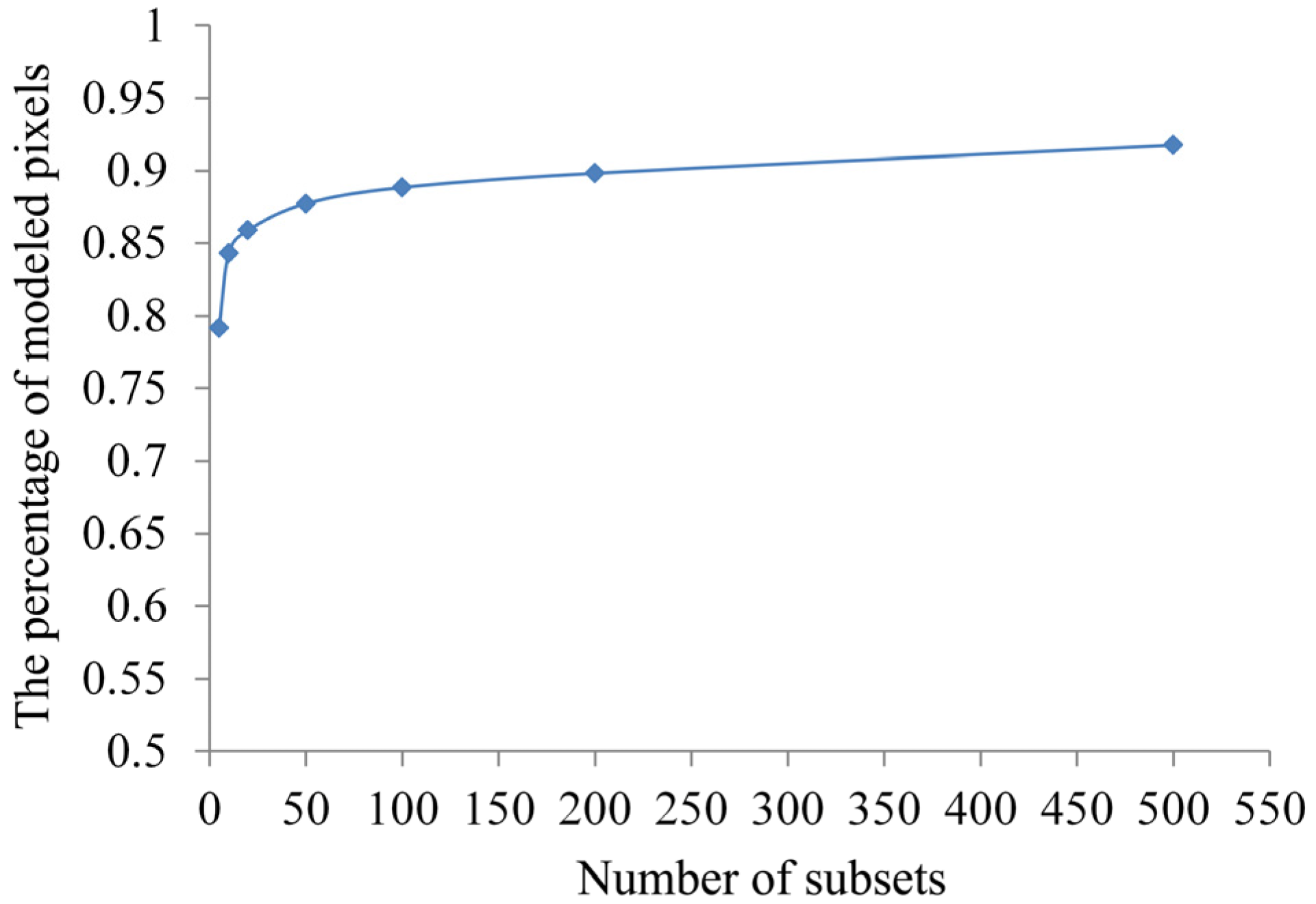
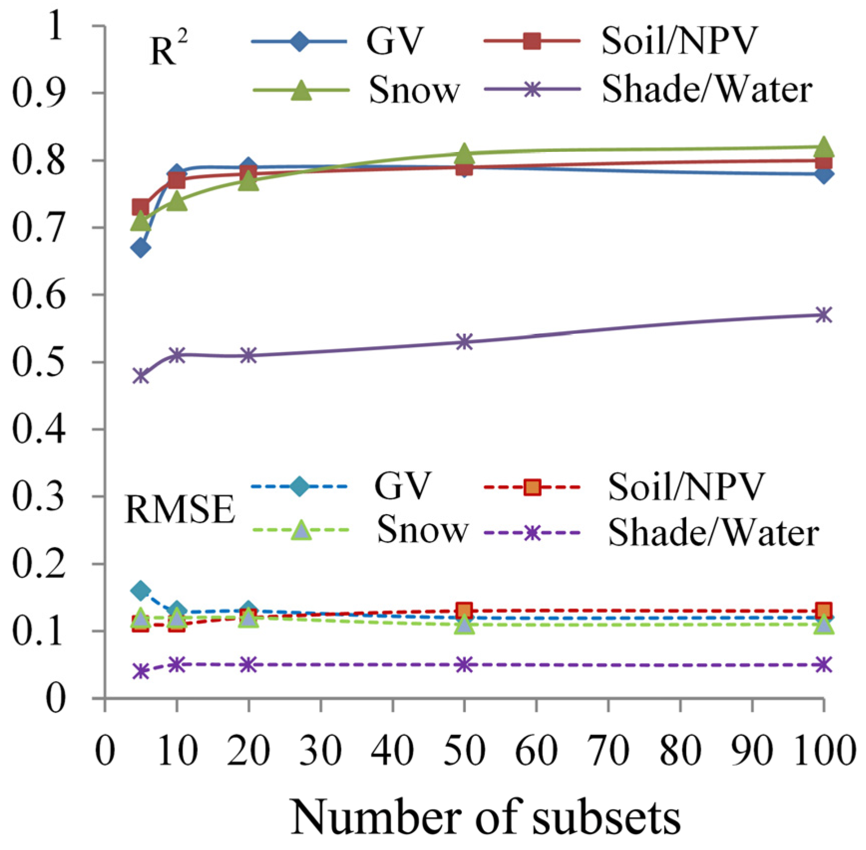
The number of subsets, n in Equation (2), is an empirical parameter, and it is determined empirically by class size, variability of spectra in a class, and spectral wavelength. In the experiment of fraction map using MODIS imagery, seven n-subset (from to 500-subset) were used to partition subsets, respectively. Although the number of the successfully modeled pixels increased with the increasing subset numbers, the accuracy of fraction mapping was not monotonically increased. The non-monotoic changes of the accuracy may indicate that increasing number of representative endmembers for MESMA possibly leads to difficulties for interpreting classification.

The previous research illustrated the RMSE of model fits decreased with increasing iterations for MESMA using the original library or representative library, and which stabled at numbers of iterations (60 to 200 iterations) for different scenario [21]. Taking into account the previous research, we have used seven n-subset to test the mapping performance of n-subset for 2-endmember MESMA, and the successfully modeled pixels of MODIS increased with increasing the numbers of subsets. The accuracies of the fraction maps presented higher values at one n-subset. To balance the accuracy and efficient, the results of experiments indicated n-20 are preferable for mapping fractions of green vegetation and soil/rock classes and n-50 are preferable for snow class.

The number of spectra in each subset may be different due to the fixed width of partition. The advantage using fixed width is to ensure predictable range of vector length, so that the spectra are can be equally sub-divided with the same length range and low variability. In order to be more representative, spectra of a class should be less variable. Otherwise, high spectral variability of a class will cause increasing errors of MESMA modeled by the representative endmembers [3]. The subset division using the vector lengths is suitable for selecting the representative endmember spectra for the classes with high albedo variability.

The computing time of fraction maps using MESMA is dependent on two factors: (1) the processing time to select representative endmembers; (2) the processing time to model MESMA using the representative endmembers. For endmember selection, the previous methods need to iteratively model the complete spectra (N spectra), which will use the N^2 time. While, the new method needs the N time due to calculation by spectral itself. For MESMA model, the processing time is dependent on the number of the representative spectra selected from the complete spectra, and less number of the representative spectra will be faster. The new endmember selection selects representative endmember faster, and the fraction map of image using less number of the representative endmembers is not only efficient but also accurate.

In this study, MODIS reflectance channels were highlighted for multiple spectral data. Our experiments indicated that vector length is an efficient metric to quantize subsets of a class in MODIS reflectance channels. Due to the discernable ability about detailed information on spectral variation, hyperspectral data expand the classification to the land cover. Future work might focus on the hyperspectral channels to expand applications of the vector length metric. Instead of using the fixed width for subset partitions, an adaptive width, dependent on the variability (deviation) of vector length, would be used to possibly improve the method using fixed width.

5. Conclusions

We test a new quantitative metric, vector length, for endmember selection. Spectra derived from reference polygon were used to compare the new method to EAR/CoB method, and a MODIS image was used to test the performance of MESMA for mapping. The comparison of representative spectra based on EAR/CoB and vector length indicated that the new selection method performed slightly better in accuracy. The number of 70 spectra selected by vector length is more efficient than the 78 spectra based on EAR/CoB. For the MODIS image experiment, the simulation accuracies of image pixels modeled by the representative endmembers were increasing, when the numbers of representative spectra increases (Figure 3). However, fractional accuracies of endmembers were not monotonically increasing (Table 7). In the experiment, the 20 subsets for class GV and soil/NPV and 50 subsets for snow performed the better accuracy of land cover fractions for MODIS reflectance channels. The RMSEs of model fits are not sensitive to the low albedo spectra [7]. Therefore, the fraction accuracy of shade/water endmembers was very low as their low albedo.

The vector length is an effective metric for dividing spectral subsets of a class and selecting representative endmembers for MESMA. The representative endmembers of image data successfully modeled all the image endmembers and image pixels. Although the image endmembers from a mountainous terrain increased the spectral variability and the uncertainties of mode fit, the better results of our image experiment presented the stability of the new method to higher spectral variability.