Article

Evaluating Different Methods for Grass Nutrient Estimation from Canopy Hyperspectral Reflectance

1
School of Resource and Environmental Science & Key Laboratory of Geographic Information System of the Ministry of Education, Wuhan University, Wuhan 430079, China
2
Faculty of Geo-Information Science and Earth Observation (ITC), University of Twente, Enschede 7500, The Netherlands
3
Key Laboratory for Geo-Environment Monitoring of Coastal Zone of the National Administration of Surveying, Mapping and Geo-Information & Shenzhen Key Laboratory of Spatial-Temporal Smart Sensing and Services & College of Life Sciences, Shenzhen University, Shenzhen 518060, China
*
Author to whom correspondence should be addressed.
Remote Sens. 2015, 7(5), 5901-5917; https://doi.org/10.3390/rs70505901
Submission received: 13 January 2015 / Revised: 15 April 2015 / Accepted: 5 May 2015 / Published: 11 May 2015

Abstract

:
The characterization of plant nutrients is important to understand the process of plant growth in natural ecosystems. This study attempted to evaluate the performances of univariate linear regression with various vegetation indices (VIs) and multivariate regression methods in estimating grass nutrients (i.e., nitrogen (N) and phosphorus (P)) with canopy hyperspectral reflectance. Synthetically considering predictive accuracy, simplicity, robustness and interpretation, the successive projections algorithm coupled with multiple linear regression (SPA-MLR) method was considered optimal for grass nutrient estimation at the canopy level, when compared with the performances of 12 statistical modeling methods, i.e., univariate linear regression with nine published VIs and three classical multivariate regression methods (stepwise multiple linear regression (SMLR), partial least squares regression (PLSR) and support vector regression (SVR)). The simple ratio index ( R 730 / R 705 , R is derivative reflectance) model had comparable performance to SPA-MLR model for P estimation. SPA-MLR provided comparable prediction accuracies with only three first derivative spectral bands for N (715, 731 and 2283 nm) and P (714, 729 and 1319 nm) estimations, compared with PLSR and SVR models, which used the full spectrum. Moreover, SPA-MLR provided robust prediction with the lowest bias values for N (−0.007%) and P (0.001%) estimations, and the fitting line between predicted and measured values was closer to the 1:1 line than the other models. Finally, most of the bands selected by SPA-MLR indirectly relate to foliar chlorophyll content, which suggests good physical interpretation.

1. Introduction

The characterization of plant nutrients, e.g., nitrogen (N) and phosphorus (P), is important to understand the process of plant growth in natural ecosystems [1] and helps to understand the foraging behavior, habitat selection and migration of some animals [2,3]. Over the last four decades, the advances in reflectance spectroscopy, airborne and satellite technology have made it feasible to be more independent of routine wet-chemistry analyses for plant nutrients, and they have provided opportunities for scientists to understand the temporal and spatial changes of plant nutrients at a landscape or regional scale [4,5,6,7,8,9]. Among these studies, univariate regression with vegetation indices (VIs) and multivariate regression methods are commonly used to extract useful information for nutrient characterization. These modeling methods provide convenient and interpretable means for researchers to understand the fundamental interaction of plant condition with radiant energy detected by multispectral or hyperspectral sensors [4,5,6,7,9,10,11,12,13,14,15,16].
Since Pearson and Miller [17] proposed the first two VIs, i.e., the ratio vegetation index (RVI) and vegetation index number (VIN) for estimating grass productivity, many followers have proposed and improved hundreds of VIs to minimize solar irradiance and soil background effects and to enhance the vegetation response further [6,11,15,18,19,20,21,22,23,24,25]. Generally, the VIs are classified into two large categories: (i) broadband VIs, which are derived from the reflectance of multispectral sensors (e.g., Landsat MSS, Landsat TM, SPOT, AVHRR and MODIS); and (ii) narrowband VIs, which are derived from the reflectance of hyperspectral sensors, including ground-based (e.g., ASD FieldSpec portable spectroradiometer), airborne (e.g., Hymap) and spaceborne (e.g., Hyperion) sensors. Some studies demonstrated that narrowband VIs could overcome the saturation problem commonly occurring for broadband VIs for biomass estimation in dense vegetation [20]. Recent studies further demonstrated the successful applications and high prediction accuracies of narrowband VIs in estimating plant nutrients (e.g., N) [6,12,13,15,21,23,24,25]. Apart from the traditional simple ratio index (SRI) and normalized difference index (NDI), which contain only two spectral bands, the three-band index (TBI) and red edge parameters (e.g., red edge position (REP)) have also been reported to result in higher prediction accuracy for nutrient estimations. For example, Tian et al. [24] and Pacheco-Labrador et al. [15] respectively compared the performances of 61 and 82 published VIs for N estimations, and they claimed their newly proposed TBIs improved prediction accuracy. However, their studies showed that these aforementioned VIs are sensitive to specific vegetation species, growth stages and study areas.
Since the early attempt at estimating the N content in sweet pepper leaves from laboratory-based reflectance with univariate regression [26], many researchers have used linear or non-linear multivariate regressions for plant nutrient estimations, such as stepwise multiple linear regression (SMLR) [5,6,8,27], partial least squares regression (PLSR) [5,9,27] and support vector regression (SVR) [14,28]. SMLR is the linear combination of several important bands selected from the whole reflectance spectra; however, it has the potential problem of over-fitting [29]. PLSR can overcome the problem of multicollinearity commonly existing between narrow hyperspectral bands, because it compresses the whole spectra into several latent variables. SVR has the advantage of extracting non-linear relationships from reflectance spectra. Although some studies reported that PLSR and SVR could improve the prediction accuracy compared with SMLR [5,27,30], such results were obtained at the expense of increasing model complexity due to the use of whole spectra for modeling. Moreover, in order to acquire higher prediction accuracy when employing the multivariate regression methods, the original reflectance spectra often require some pre-processing methods, such as first derivative analysis [9,31], absorbance [5], continuum-removal [6,8] or water-removal analysis [27]. However, the different choice of spectral pre-processing methods may yield completely different prediction results. Therefore, the choice of pre-processing and multivariate regression methods makes it difficult to balance between model accuracy and simplicity.
The successive projections algorithm combined with multiple linear regression (SPA-MLR) proved to be a time-saving and robust method for multivariate calibration [32], and it has been successfully applied to many fields of research, such as spectroscopic chemical analysis [33,34] and grass nutrient assessment [31]. SPA selects informative wavelengths by using simple operations in a vector space to minimize variable collinearity [32]. Cui et al. [31] reported that SPA-MLR outperformed PLSR with higher prediction accuracy and better model simplicity and confirmed the advantage of SPA-MLR in grass nutrient estimation using laboratory-based reflectance.
However, it is still unknown whether SPA-MLR is comparable to PLSR in grass nutrient estimation with canopy reflectance data, because canopy spectra are popularly used in vegetation studies, and they can better characterize the actual status of vegetation than leaf spectra. Little guidance and few comprehensive comparative studies have been offered to choose among the aforementioned methods (i.e., univariate regression with VIs, multivariate regression methods and SPA-MLR) for estimating grass nutrients at the canopy level. Moreover, it also remains unknown whether the optimal method is consistent in estimating different nutrient elements.
The performance of a statistical model using hyperspectral reflectance is often evaluated by predictive accuracy, i.e., determination coefficient (R2), root mean square error (RMSE) and ratio of prediction to deviation (RPD) [14,20,27,31,35,36]. However, little information of model simplicity, robustness and interpretation can be gained from the predictive accuracy. A simple model should confirm the notion of Occam’s razor [37]; a robust model should be unbiased and transferable (both temporally and spatially) [29,38]; and an interpretable model should consider physical meaning for the included spectral bands [10,15,18]. Therefore, it is recommended to synthetically consider predictive accuracy, simplicity, robustness and interpretation for evaluating model performance.
Carex cinerascens is a wetland grass species widely distributed in Poyang Lake, China, and it is the main food for some over-wintering birds, such as the swan goose (Anser cygnoides) and white-fronted goose (A. albifrons albifrons) [39]. This study aimed to evaluate the performances of univariate linear regression with nine published VIs, three classical multivariate regression methods (SMLR, PLSR and SVR) and SPA-MLR in estimating the nutrients (N and P) of C. cinerascens with canopy hyperspectral reflectance. Such comparison might help to understand their comprehensive performance from the perspective of model accuracy, simplicity, robustness and interpretation and would provide guidance in selecting the optimal method for estimating plant nutrients at various levels.

2. Material and Methods

2.1. Sampling Design and Canopy Spectral Measurements

The study was carried out in Poyang Lake (28°52′21″−29°06′46″N, 116°10′24″−116°23′50″E), Jiangxi Province, China. As the largest freshwater lake in China, Poyang Lake is an important wetland in the world for bird over-wintering. In order to obtain a large variation of N and P contents for modeling, field sampling was designed in different growth stages of C. cinerascens. Two field surveys were carried out from 4−7 December 2012 (vegetative stage) and from 10−15 April 2013 (heading stage), respectively, when Poyang Lake was in dry seasons. In each field survey, nine sites (150 × 150 m), which could be physically measured without interference caused by deep water, were randomly arranged within large areas of C. cinerascens. At each site, four to eight plots (1 × 1 m) were randomly laid out to keep at least 30 m apart between any two plots. Due to dense canopy cover (nearly 100%), very little soil beneath C. cinerascens in each plot could be seen from above the canopy. The canopy spectra and leaf samples for 66 and 71 plots were measured and collected in 2012 and 2013, respectively, following the same procedure: (i) the longitude and latitude coordinates at each plot were obtained using a global position system receiver (Garmin Ltd., Lenexa, KS, USA); (ii) prior to each spectral measurement, a calibrated white Spectralon panel was used to minimize the effect of changes of solar irradiance and atmospheric conditions on canopy reflectance; (iii) ten successive spectra (350–2500 nm, 2151 spectral bands) were measured 1 m above the canopy at nadir position using an ASD FieldSpec® 3 (spectral resolution: 3 nm at 700 nm and 10 nm at 1400/2100 nm; sampling interval: 1.4 nm at 350–1050 nm and 2 nm at 1000–2500 nm) portable spectroradiometer (Analytical Spectral Devices, Inc., Boulder, CO, USA) with a field of view of 10°; (iv) after spectral measurement, the subplots of 0.25 × 0.25 m in the four corners and center of each plot were harvested by clipping leaves (5 cm above the ground) and merged; and (v) the merged fresh leaves were immediately put into a labeled sample bag for their chemical analyses.

2.2. Chemical Analysis

The collected leaf samples were dried at 70 °C for 24 h in an oven, ground with an agate mortar and passed through a 65-mesh sieve (0.25 mm). The dried and ground samples were initially pre-processed by HCLO4−H2SO4 digestion. Following digestion, N content (%) was measured with the semi-micro Kjeldahl method [40], and P content (%) was determined using the MO-Sb (molybdenum-antimony) colorimetric method [41]. To ensure measurement accuracy, certified house reference materials and reagent blanks were used during chemical analyses.

2.3. Spectral Pre-Processing

For each sampling plot, the collected ten successive spectra were averaged as the final spectrum. Due to the large noises at edges and the water absorption regions of each spectrum, the raw canopy spectra were reduced from 2151 wavebands (350–2500 nm) to 1603 wavebands, including three spectral portions (i.e., 400−1350, 1450−1750 and 2050−2400 nm). Because some vegetation indices (VIs), such as red edge position (REP), use 1st derivative spectra, the spectra were then subjected to first derivative analysis using the Savitzky–Golay filter to reduce the effects of multiple scattering of radiation [12,42]. The spectral pre-processing and subsequent modeling were implemented with PLS_Toolbox 7.3 (http://www.eigenvector.com/software/pls_toolbox.htm) based on MATLAB 7.11 (The MathWorks, Inc., Natick, MA, USA).

2.4. Modeling Methods

2.4.1. Univariate Linear Regression with VIs

In this study, we employed nine narrowband VIs (Table 1) that were recently proposed for N or N-related component estimations to establish univariate linear relationships with N and P contents. These VIs were derived from canopy hyperspectral reflectance measured by spectroradiometers. Apart from TBI3 applied in forest ecosystem, the other eight VIs were applied in farmland ecosystem. The VIs can mainly be classified into four groups: simple ratio index (SRI), normalized difference index (NDI), three-band index (TBI) and red edge parameters, e.g., red edge position (REP). To date, very few studies have used VIs for P estimation [43,44]. Therefore, univariate linear regression models with these VIs (the name of the VI was noted as the univariate linear regression model with the VI for simplicity) were built for the N and P estimations of grass species (e.g., C. cinerascens).
Table 1. Nine published vegetation indices (VIs) for N or N-related component estimation using canopy hyperspectral reflectance. SRI, simple ratio index; NDI, normalized difference index; TBI, three-band index.
VIsFormulaPlant SpeciesR2ValLiterature
SRI1 R 990 / R 720 Wheat0.847Yao et al. [23]
SRI2 R 743 / R 1316 Sugarcane0.760Abdel-Rahman et al. [12]
SRI3 R 730 / R 705 Corn0.706Corp et al. [22]
NDI1 R 860 R 720 R 860 + R 720 Wheat0.836Yao et al. [23]
NDI2 R 750 R 705 R 750 + R 705 Corn0.672Corp et al. [22]
TBI1 R 705 / ( R 717 + R 491 ) Rice0.830Tian et al. [24]
TBI2 R 924 R 703 + 2 R 423 R 924 + R 703 2 R 423 Rice0.866Wang et al. [25]
Wheat0.883
TBI3 R 1310 / ( R 1720 + R 730 ) Holm oak0.760Pacheco-Labrador et al. [15]
REP c 1 c 2 m 1 m 2 Maize Rye0.860Cho and Skidmore [21]
0.820
REP, red edge position extracted by linear extrapolation technique. R λ   and R λ represent the original and 1st derivative reflectance at λ nm, respectively. c1 and m1 represent the intercept and slope of the far-red (680–700 nm) line, respectively; c2 and m2 represent the intercept and slope of the NIR (725–760 nm) line, respectively. R2Val, determination coefficient of validation.

2.4.2. Classical Multivariate Regression Methods

Three multivariate regression methods (SMLR, PLSR and SVR) have been popularly employed for N and P estimations of plants at leaf, canopy and landscape levels (Table 2). These methods often employ pre-processed spectra (e.g., continuum-removed, absorbance, 1st derivative and water-removed spectra) for modeling to improve predictive accuracy.
Table 2. A list of some literature on N and P estimations using multivariate regression methods. SMLR, stepwise multiple linear regression; PLSR, partial least squares regression; SVR, support vector regression.
MethodReflectance Spectra UsedN (R2Val | RMSEVal)P (R2Val | RMSEVal)Literature
SMLRCanopy, continuum-removed0.700–0.7600.310–0.460Mutanga et al. [6]
SMLRLeaf, absorbance 0.232 | 0.087%Bogrekci and Lee [5]
SMLRImage, continuum-removed0.210 Ullah et al. [8]
SMLRCanopy, 1st derivative 0.590 | 0.450%0.250 | 0.080%Ramoelo et al. [27]
SMLRCanopy, water-removed0.870 | 0.250%0.640 | 0.060% Ramoelo et al. [27]
PLSRCanopy, 1st derivative0.590 | 0.450%0.470 | 0.070%Ramoelo et al. [27]
PLSRCanopy, water-removed 0.840 | 0.280%0.430 | 0.070%Ramoelo et al. [27]
PLSRLeaf, absorbance 0.425 | 0.073%Bogrekci and Lee [5]
PLSRCanopy, 1st derivative 0.830 | 0.210%0.770 | 0.050%Sanches et al. [9]
SVRImage, original 0.030–0.673 Karimi et al. [28]
SVRLeaf, 1st derivative0.706 | 0.521%0.722 | 0.073%Zhai et al. [14]
SVRLeaf, original 0.197 | 0.946%0.458 | 0.097%Zhai et al. [14]
RMSEVal, root mean square error of validation. The continuum-removed, absorbance, 1st derivative and water-removed spectra were the transformations of the original reflectance spectra. The data in Ullah et al. [8] and Karimi et al. [28] were collected by spaceborne and airborne sensors, respectively; the data in the other studies were measured by spectroradiometers.
SMLR starts with no selected variable (wavelength) and searches the best single wavelength at each iteration based on the highest F-statistic value or the lowest p-value [12]. SMLR computes the F-statistic and p-values for each wavelength, and it removes irrelevant wavelengths based on predefined removal F-statistic or p-values. The procedure stops at the n-th iteration when n wavelengths are selected. The entry and removal of p-values were set at 0.05 and 0.10 based on empirical settings, respectively. To minimize the over-fitting problem of SMLR, the M/N ratio (M = the number of selected wavelengths, N = the number of calibration samples) suggested by Thenkabail et al. [11] and variation inflation factor (VIF) described by Neter et al. [45] were employed. The M/N ratio and VIF did not exceed 0.15–0.20 and 5–10, respectively. The optimum number of selected wavelengths was determined by the best SMLR model with the highest prediction accuracy based on the test set.
PLSR brings together the advantages of principal component analysis (PCA), canonical correlation analysis (CCA) and MLR [46]. Unlike PCA, PLSR compresses predictor variables into several latent variables (LVs) to capture both of the greatest variance of predictor variables and the maximum correlation between the LV scores and dependent variables (e.g., N or P contents) [7,29,46]. The details of PLSR can be found in Geladi and Kowalski [46]. The optimum number of LVs was determined by leave-one-out cross-validation procedure. To prevent collinearity and over-fitting, the root mean square error of cross-validation (RMSECV) should be reduced by >2% when adding an extra LV to the PLSR model [7,47].
Unlike SMLR and PLSR, SVR is a non-linear statistical learning technique. SVR computes a linear regression function in a high dimensional feature space, in which the input data are mapped by a non-linear function [48]. Moreover, it optimizes the generation error in order to obtain the best generalized performance on a limited number of support vectors (SVs) [48,49]. The details of SVR can be found in Smola and Schölkopf [48]. The optimization process was tuned by a systematic grid search of the parameters using five-fold cross-validation [29].

2.4.3. SPA-MLR

The successive projections algorithm (SPA) proposed by Araújo et al. [32] is a forward selection method in order to minimize variable collinearity. In a nutshell, SPA starts with one wavelength and selects a new one at each iteration by using projection operators in a vector space until reaching the predefined number of wavelengths. The new selected wavelength has the maximum projection value on the orthogonal subspace of the previous selected wavelengths [50]. Unlike genetic algorithm (GA), which is a popular variable selection method based on survival of fittest theory, SPA is a deterministic search technique, and it is more robust according to the choice of validation samples [32]. MLR was employed to establish the relationship between the wavelengths selected by SPA and dependent variables (N or P contents). To prevent over-fitting and to obtain the best SPA-MLR model, the maximum and optimum number of selected wavelengths were determined following the same method used for SMLR (see Section 2.4.2). SPA was implemented using SPA_GUI 1.0 (www.ele.ita.br/~kawakami/spa) based on MATLAB 7.11 (The MathWorks, Inc., Natick, MA, USA).

2.5. Model Development

For N or P estimation using the 13 aforementioned modeling methods, preliminary experiments showed that the predictive accuracies were very poor (R2 < 0.30) with the two original datasets (Table 3) for the training set and test set; this might because the nutrient contents in the original datasets had a narrow range and imbalanced statistical distribution [7]. Thus, the original datasets collected over two growth stages were combined into a single dataset, and its N and P contents were sorted from the lowest to highest values, respectively. The combined dataset was then partitioned into two datasets following the partitioning strategy given by Kemper and Sommer [35]. The odd-numbered samples were selected as the training (or calibration) set, while the even-numbered samples as the test (or validation) set (Table 3). The new training set and test set had similar statistical distribution of nutrient contents, and they provided a much wider range and higher coefficient of variation of nutrient contents than the original datasets. To some extent, this data partitioning could avoid the unbiased estimation. For each modeling method (see Section 2.4) in N and P estimations, the training set was used for model calibration and cross-validation, and the test set was applied for model validation.
In this study, three VIs (SRI2, SRI3 and REP), three multivariate regression methods (SMLR, PLSR and SVR) and the SPA-MLR method employed the 1st derivative spectra for modeling, while the other six VIs (i.e., SRI1, NDI1, NDI2, TBI1, TBI2 and TBI3) used the original spectra following the original formula. Therefore, a total of 13 models were established for N and P estimations, respectively.
Following the suggestion of Wise et al. [29], prior to modeling, the dependent variables (N or P contents) and independent variables (VIs or 1st derivative spectra) were processed with the autoscaling method to obtain a uniform dimension. This method uses mean-centering followed by dividing each variable by the standard deviation of the variables [29]. The determination coefficient of cross-validation and validation (R2CV and R2Val), the root mean square error of cross-validation and validation (RMSECV and RMSEVal), the ratio of prediction to deviation (RPD, the ratio of the standard deviation of the reference values in the test set to RMSEVal) and the bias for validation were calculated for each model. Further, due to using the whole spectra for modeling, PLSR and SVR had much more complicated model equations than the VIs, SMLR and SPA-MLR, which employed a limited number of predictor variables. Thus, only the optimum number of LVs and SVs was reported for PLSR and SVR models, respectively.
Table 3. Descriptive statistics of N and P contents.
NutrientDatasetnRange (%)Mean (%)CV (%)
Original dataNDecember 2012661.73−3.082.4414.56
April 2013711.00−2.071.5912.98
PDecember 2012660.17−0.410.2817.51
April 2013710.08−0.200.1613.57
Data partitioningNTraining set691.00−3.082.0026.03
Test set681.12−3.062.0025.38
PTraining set690.08−0.410.2233.06
Test set680.18−0.370.2231.68
CV, coefficient of variation, the ratio of the standard deviation to the mean value; n, the number of samples.

2.6. Model Comparison

The 13 statistical models for N estimation were compared based on their prediction performances (R2Val, RMSEVal, RPD and bias), respectively. Afterwards, the best-performing VI and classical multivariate regression models with the highest predictive accuracy were chosen to be compared with the SPA-MLR model for N estimation, according to the slope and intercept values for the fitting line between predicted and measured values. The aforementioned methods were employed for comparison of the 13 statistical models for P estimation. Moreover, in order to synthetically explore the significant differences between SPA-MLR and the other modeling methods for nutrient (N and P) estimation, one-way analysis of variance (ANOVA) using the least squares difference (LSD) method was performed considering the mean R2Val values of the 13 methods for N and P estimations.

3. Results

3.1. Comparison of the Modeling Methods for N Estimation

Among the aforementioned 13 models for N estimation (Table 4), the PLSR (R2Val = 0.747, RMSEVal = 0.248%, RPD = 2.03), SVR (R2Val = 0.740, RMSEVal = 0.254%, RPD = 1.98) and SPA-MLR (R2Val = 0.738, RMSEVal = 0.258%, RPD = 1.95) models provided higher validation accuracies than the other ten models. SPA-MLR with three first derivative spectral bands (715, 731 and 2283 nm) provided the lowest bias value (−0.007%) among the 13 models, while SVR and PLSR using the full-spectrum (1603 bands) provided about seven-times higher absolute bias values than SPA-MLR. Moreover, the SRI3 model (R2Val = 0.705, RMSEVal = 0.275%, RPD = 1.83) outperformed the other eight VI models considering predictive accuracy. Additionally, the VIs (TBI1, TBI2 and TBI3) with three bands did not perform better than the VIs (SRI1, SRI2, SRI3, NDI1 and NDI2) with two bands in predictive accuracy.
Table 4. Cross-validation and validation results of 13 modeling methods to estimate N contents at the canopy level. SPA, successive projections algorithm.
Modeling MethodsModel EquationCross-Validation (n = 69)Validation (n = 68)
R2CVRMSECVR2ValRMSEValbiasRPD
SRI1 Y N = 0.815 × S R I 1 0.6490.3060.6390.303−0.0281.66
SRI2 Y N = 0.816 × S R I 2 0.6530.3040.6190.315−0.0311.60
SRI3 Y N = 0.848 × S R I 3 0.7090.2780.7050.275−0.0321.83
NDI1 Y N = 0.829 × N D I 1 0.6750.2940.6740.289−0.0331.74
NDI2 Y N = 0.828 × N D I 2 0.6710.2960.6500.301−0.0441.67
TBI1 Y N = 0.770 × T B I 10.5800.3350.4800.367−0.0421.37
TBI2 Y N = 0.825 × T B I 2 0.6680.2980.5990.320−0.0261.57
TBI3 Y N = 0.556 × T B I 3 0.2600.4470.3540.406−0.0181.24
REP Y N = 0.843 × R E P 0.6990.2830.6920.282−0.0391.78
SMLR Y N = 0.403 × R 684   0.576 × R 1177   0.193 × R 1270   0.295 × R 2306   0.7080.2790.6700.2910.0311.73
PLSR4 LVs0.5380.3630.7470.2480.0482.03
SVR69 SVs0.5940.3340.7400.2540.0511.98
SPA-MLR Y N = 0.973 × R 715   + 1.327 × R 731     0.181 × R 2283   0.7100.2780.7380.258−0.0071.95
YN, N content (%). The units of RMSECV, RMSEVal and bias are %.
Figure 1. (af) Scatter plots of measured and predicted values based on the best-performing VI (first column), best-performing multivariate regression (second column) and SPA-MLR (third column) model for N and P estimations, respectively. The dotted and solid lines present the 1:1 line and linear fitting line between measured and predicted values, respectively. The ellipse denotes the 95% confidence ellipse.
Remotesensing 07 05901 g001
Among the best-performing VI (SRI3) (Figure 1a), best-performing multivariate regression (PLSR) (Figure 1b) and SPA-MLR (Figure 1c), the SPA-MLR model provided a higher slope value (0.772) and lower intercept value (0.449) for the fitting line between predicted and measured values than the SR3 model (slope = 0.711, intercept = 0.545). In addition, the SPA-MLR model provided a lower slope value than the PLSR model (slope = 0.789). There were two sample points outside or on the verge of the 95% confidence ellipse for all three models.

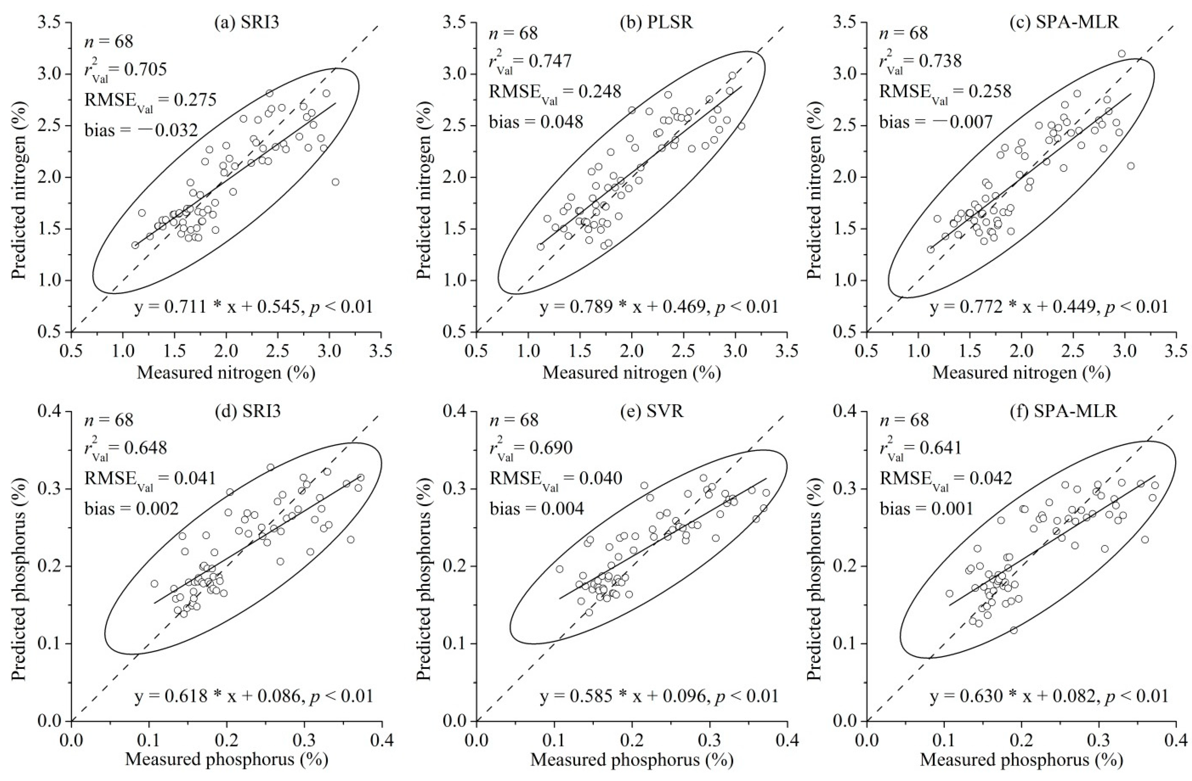
3.2. Comparison of the Modeling Methods for P Estimation

Among the aforementioned 13 models for P estimation (Table 5), the SVR (R2Val = 0.690, RMSEVal = 0.040%, RPD = 1.77), SR3 (R2Val = 0.648, RMSEVal = 0.041%, RPD = 1.70) and SPA-MLR (R2Val = 0.641, RMSEVal = 0.042%, RPD = 1.66) models provided much higher validation accuracies than the other ten models. Moreover, SPA-MLR provided the lowest bias value (0.001%) among the 13 models. Using the same number of first derivative spectral bands, the SPA-MLR model (714, 729 and 1319 nm) had 9.95% and 8.50% higher R2Val and RPD values than the SMLR model (595, 1087 and 1181 nm), respectively. Besides, consistent with the results of N estimations, the SRI3 model also achieved the highest predictive accuracy among the nine VIs, and the VIs (SRI1, SRI2, SRI3, NDI1 and NDI2) with two bands still outperformed the VIs (TBI1, TBI2 and TBI3) with three bands.
Among the best-performing VI (SRI3) (Figure 1d), best-performing multivariate regression (SVR) (Figure 1e) and SPA-MLR (Figure 1f) models, the SPA-MLR model provided a higher slope (0.630) and lower intercept (0.082) than the SRI3 model (slope = 0.618, intercept = 0.086) and the SVR model (slope = 0.585, intercept = 0.096). In addition, there were two points outside or on the verge of the 95% confidence ellipse for the SPA-MLR model, while three points for the SRI3 and SVR models.
Table 5. Cross-validation and validation results of 13 modeling methods to estimate P contents at the canopy level.
Modeling MethodsModel EquationCross-Validation (n = 69)Validation (n = 68)
R2CVRMSECVR2ValRMSEValbiasRPD
SRI1 Y P = 0.811 × S R I 1 0.6460.0430.6050.0440.0041.58
SRI2 Y P = 0.753 × S R I 2 0.5450.0490.6010.046−0.1131.55
SRI3 Y P = 0.823 × S R I 3 0.6660.0420.6480.0410.0021.70
NDI1 Y P = 0.821 × N D I 1 0.6630.0420.6090.0440.0051.58
NDI2 Y P = 0.790 × N D I 2 0.6080.0460.5910.0450.0031.54
TBI1 Y P = 0.673 × T B I 10.4170.0560.4230.0530.0011.31
TBI2 Y P = 0.764 × T B I 2 0.5680.0480.5570.0460.0021.51
TBI3 Y P = 0.556 × T B I 3 0.4030.0560.3070.0620.0121.12
REP Y P = 0.843 × R E P 0.6370.0440.6180.0430.0041.62
SMLR Y P = 0.362 × R 595   0.260 × R 1087   0.401 × R 1181   0.6210.0450.5830.0450.0061.53
PLSR2 LVs0.5590.0480.5470.0470.0031.48
SVR60 SVs0.5990.0460.6900.0400.0041.77
SPA-MLR Y P = 1.006 × R 714   + 1.579 × R 729 + 0.190 × R 1319   0.6200.0450.6410.0420.0011.66
YP, P content (%).The units of RMSECV, RMSEVal and bias are %.

3.3. Differences in Model Accuracy

In order to explore the differences between SPA-MLR and the other 12 modeling methods in predictive accuracy, a one-way analysis of variance (ANOVA) of the R2Val values for N and P estimations was performed (Table 6). The SPA-MLR model (Number 13) differed from the TBI1 (Number 6) and TBI3 (Number 8) models at a significance level of 0.05. However, the other 10 models had no significant differences with the SPA-MLR model (Number 13), because the p-values were greater than 0.05.

4. Discussion

4.1. Comparison of Model Performance

Although some studies have made comparisons between different multivariate regression methods or spectral pre-processing methods in estimating biochemical components in plant leaves [14,27,31], this study is a further attempt to comprehensively compare the performances of 13 statistical modeling methods for grass (e.g., C. cinerascens) nutrient (N and P) estimation using canopy hyperspectral reflectance. Univariate linear regression with nine published VIs, three classical multivariate regression methods (SMLR, PLSR and SVR) and the SPA-MLR method were compared, and the results comprehensively showed that SPA-MLR was an optimal method from the perspectives of prediction accuracy, model simplicity and robustness. Firstly, despite SPA-MLR having no significant difference with the full-spectrum PLSR and SVR in prediction accuracy at the 0.05 level (Table 6), it substantially decreased model complexity due to the use of only three bands for N and P estimations. Secondly, although SMLR used a similar number of bands to SPA-MLR for modeling, the former method achieved weaker prediction accuracy than the latter. Such a result supports the inference that SPA outperformed the stepwise selection method in choosing the most informative wavelengths from canopy spectra for N and P estimations. Thirdly, SPA-MLR showed better model robustness, because SPA-MLR provided the lowest bias values, both for N and P estimations, and the fitting line between predicted and measured values was closer to 1:1 line than SRI3 and SVR (Figure 1), though the best-performing VI (SRI3) had similar model simplicity and predictive accuracy as SPA-MLR.
Compared with the published literature, using the three classical multivariate regression methods (Table 2) for N (R2Val = 0.030−0.870) and P (R2Val = 0.232−0.770) estimations and the VIs (Table 1) for N estimation (R2Val = 0.672−0.883), the SPA-MLR method in this study exhibited an average and acceptable prediction ability for N (R2Val = 0.738) and P (R2Val = 0.641) estimations. According to the interpretation of R2 given by Williams [51], the SPA-MLR model using first derivative canopy spectra provided approximate quantitative prediction for N (0.66 < R2Val < 0.81), as well as the possibility to distinguish between high and low values for P (0.50 < R2Val < 0.65). The same modeling method was employed by Cui et al. [31], who employed the first derivative leaf spectra and achieved much poorer prediction power for crude protein (multiplying the N content by a factor of 6.25) (R2Val < 0.50) and P (R2Val < 0.50) in C. cinerascens leaves than this study, which suggests an unsuccessful estimation for SPA-MLR using leaf spectra [51]. Such an evident difference of predictive accuracy considering the same modeling method and plant species could be interpreted as the canopy spectra contained stronger spectral responses and more detailed information of biochemical contents than leaf spectra to characterize vegetation status. Similar results were reported by Bian et al. [52], who demonstrated that the spectra at the canopy level achieved higher predictive accuracy than that at the leaf level for estimating vegetation biochemical content.
Table 6. One-way analysis of variance (ANOVA) of the R2Val values between SPA-MLR and the other 12 modeling methods in N and P estimations.
Model Sequence NumberMean Difference (I−J)p-Value95% Confidence Interval
IJLower BoundUpper Bound
1310.0680.283−0.0600.195
20.0800.208−0.0480.207
30.0130.834−0.1150.141
40.0480.441−0.0800.176
50.0690.272−0.0590.197
60.2380.0010.1100.366
70.1120.083−0.0160.239
80.3590.0000.2310.487
90.0350.579−0.0930.162
100.0430.495−0.0850.170
11−0.0260.681−0.1530.102
120.0250.693−0.1030.152
The sequence number 1−9 respectively represents SRI1, SRI2, SRI3, NDI1, NDI2, TBI1, TBI2, TBI3 and REP; 10−13 represents SMLR, PLSR, SVR and SPA-MLR.
Consistent with the finding of Cui et al. [31], this study demonstrated the outperformance of SPA-MLR for plant nutrient estimation from the leaf to canopy level. Such performance could be explained by SPA choosing a small number of spectral bands with a minimum of collinearity, obtained by employing projection operators in a vector space [32]. Moreover, the simplicity of the SPA-MLR model contributed to its outperformance, because MLR yielded models that were easier for interpretation than the full-spectrum PLSR and SVR methods. Apart from the successful application in monitoring plant nutrient status in this study, some studies also confirmed the benefit of SPA-MLR from the aspect of spectroscopic chemical analysis, such as the determination of phenolic compounds in sea water [33] and the organic acids of plum vinegar [34].
The best-performing VI (SRI3) for N estimation tested in this study had comparable predictive accuracy to the poorest-performing VI (NDI2 and SRI3) reported in the references in Table 1. Such inconsistencies could be interpreted by the VIs being sometimes insensitive to N status due to variation across vegetation species, growth stages, study regions and even hyperspectral sensors [13,15,23,24]. However, we could not claim that the nine VIs tested in this study were unsuccessful for N estimation. For example, the SRI3, NDI1 and REP provided approximate quantitative prediction for N estimation (0.66 < R2Val < 0.81), and the SRI1, SRI2, NDI2 and TBI2 provided the possibility to distinguish between high and low values (0.50 < R2Val < 0.65) (Table 4) according to the interpretation of R2 given by Williams [51]. The estimation results of the seven VIs (SRI1, SRI2, SRI3, NDI1, NDI2, TBI2 and REP) used in this study indicate that these VIs might have some degree of transferability from crop species (e.g., wheat, rice and corn) to grass species (e.g., C. cinerascens) for N estimation. Undeniably, several studies claimed that some published VIs had poor application for N estimation. For example, Pacheco-Labrador et al. [15] demonstrated that only 16 out of the 82 published VIs achieved R2 > 0.50, and the other 66 VIs suggested unsuccessful estimation for N (R2 < 0.50). Such disagreement with the findings of this study might be because many empirical published VIs, e.g., blue/green pigment indices, pigment-specific simple ratio and pigment-specific normalized difference, were developed based on broadband wavelengths from space-borne or air-borne sensors in relation to pigment (chlorophyll, carotenoids and xanthophyll) content. However, the VIs (Table 1) tested in this study were developed by systematically searching for the most sensitive combinations of two or three narrowband wavelengths that directly relate to N content. In addition, despite few studies focusing on VIs for P estimation, this study demonstrated that the aforementioned seven VIs could be used for P estimation in C. cinerascens-dominated ecosystems (0.50 < R2Val < 0.65) (Table 5).

4.2. Interpretation of the SPA-MLR Model

Apart from the acceptable predictive ability obtained from the SPA-MLR method, the simplicity (using only three first derivative spectral bands) of this method (Table 4 and Table 5) confirms the notion of Occam’s razor [37]. The bands of 715 and 731 nm for N estimation and the bands of 714 and 729 nm for P estimation were located in the red edge region (680−750 nm). The vegetation reflectance in this region is caused by the strong absorption in the red wavelengths due to chlorophyll and by the high reflectance in the near-infrared (NIR) wavelengths due to leaf internal (mesophyll) scattering [15,21]. Because of the low contents of P in leaves and its weak influence on leaf reflectance, there were no evident absorption features of P [10,27]. Further, plant N content strongly relates to chlorophyll content [15,25]. Therefore, the aforementioned four bands could be considered as indicators for N and P status and indirectly relate to the chlorophyll content of leaves. These bands were consistent with the wavelengths contained in the VIs tested in this study (Table 1). For example, Tian et al. [24] found that the band of 717 nm was sensitive to N estimation in rice, and Corp et al. [22] claimed that the band of 730 nm contributed to monitoring nitrogen-driven carbon uptake in field corn. Moreover, the location of sensitive wavelengths for N and P estimations in this study confirms the results from other literature. For example, Vis, such as R 715 / R 705 proposed by Vogelmann et al. [19], showed that the band of 715 nm was a significant wavelength for chlorophyll estimation in sugar maple leaves. Yoder and Pettigrew-Crosby [4] further found that the band of 730 nm contributed to the estimation of N and chlorophyll of big leaf maple at the canopy level. Ramoelo et al. [27] demonstrated that the 732-nm band selected by SMLR was an important wavelength for estimating savanna grass N concentration.
The band of 2283 nm for N estimation is related to foliar starch and cellulose concentrations, which is assigned to C−H stretch or CH2 deformation [10]. This band was not the existing absorption features of N [10] or the sensitive band for N estimation found in previous references. One possible reason is that most of the absorption features of foliar N content are related to other major chemical elements of leaves, and the absorption features of these elements are overlapping. Another possible reason relates to the selection process of the SPA-MLR algorithm, which chose the important wavelengths strongly correlated with foliar N with little consideration of the specific physical meaning. The band of 1319 nm for P estimation was found to be sensitive for N estimation [12]. This indicates that P estimation might be related to foliar N content, which is supported by the strong correlation between N and P (i.e., Pearson’s correlation coefficient, r = 0.828, p < 0.01). Kawamura et al. [53] and Sanches et al. [9] also proposed the correlation between N and P and the potential reason for similar spectral regions being identified for N and P estimation.

5. Conclusions

This study compared the performances of univariate linear regression with nine published VIs (i.e., three SRIs, two NDIs, three TBIs and REP), three classical multivariate regression methods (i.e., SMLR, PLSR and SVR) and the SPA-MLR method in estimating the N and P contents of C. cinerascens leaves using field-based canopy hyperspectral reflectance. The following conclusions could be drawn from this study:
  • The SPA-MLR method had the optimal performance in both N and P estimations synthetically considering model accuracy, simplicity, robustness and interpretation, and the SRI3 model had comparable performance to the SPA-MLR model in P estimation
  • The sensitive spectral bands employed by SPA-MLR method for N (715 and 731 nm) and P (714 and 729 nm) estimations were indirectly related to foliar chlorophyll content.
  • Apart from two VIs (TBI1 and TBI3) that provided unsuccessful N and P estimations (R2Val < 0.50), the other seven VIs (SRI1, SRI2, SRI3, NDI1, NDI2, TBI2 and REP) had the potential to be applied to grass species (e.g., C. cinerascens).
This study provides guidance for extracting sensitive wavelengths for N and P estimation from canopy spectra, which is helpful for understanding the predictive mechanism of grass nutrient estimation at the canopy level.

Acknowledgments

This study was supported by the National Natural Science Foundation of China (Grant No. 41171290) and the China Scholarship Council (CSC).

Author Contributions

Junjie Wang analyzed the data, reviewed the literature and prepared the manuscript. Tiezhu Shi took part in the fieldwork. Guofeng Wu, Tiejun Wang and Andrew K. Skidmore developed the research plan. All authors contributed equally to the editing of the manuscript.

Conflicts of Interest

The authors declare no conflict of interest.

References

  1. Ingestad, T.; Lund, A.B. Theory and techniques for steady state mineral nutrition and growth of plants. Scand. J. For. Res. 1986, 1, 439–453. [Google Scholar] [CrossRef]
  2. Van der Graaf, A.; Stahl, J.; Veen, G.; Havinga, R.; Drent, R. Patch choice of avian herbivores along a migration trajectory—From Temperate to Arctic. Basic Appl. Ecol. 2007, 8, 354–363. [Google Scholar]
  3. Van Gils, J.A.; Dekinga, A.; van den Hout, P.J.; Spaans, B.; Piersma, T. Digestive organ size and behavior of red knots (Calidris canutus) indicate the quality of their benthic food stocks. Isr. J. Ecol. Evol. 2007, 53, 329–346. [Google Scholar]
  4. Yoder, B.J.; Pettigrew-Crosby, R.E. Predicting nitrogen and chlorophyll content and concentrations from reflectance spectra (400–2500 nm) at leaf and canopy scales. Remote Sens. Environ. 1995, 53, 199–211. [Google Scholar] [CrossRef]
  5. Bogrekci, I.; Lee, W. Spectral phosphorus mapping using diffuse reflectance of soils and grass. Biosyst. Eng. 2005, 91, 305–312. [Google Scholar] [CrossRef]
  6. Mutanga, O.; Skidmore, A.; Kumar, L.; Ferwerda, J. Estimating tropical pasture quality at canopy level using band depth analysis with continuum removal in the visible domain. Int. J. Remote Sens. 2005, 26, 1093–1108. [Google Scholar] [CrossRef]
  7. Darvishzadeh, R.; Skidmore, A.; Schlerf, M.; Atzberger, C.; Corsi, F.; Cho, M. LAI and chlorophyll estimation for a heterogeneous grassland using hyperspectral measurements. ISPRS J. Photogramm. Remote Sens. 2008, 63, 409–426. [Google Scholar] [CrossRef]
  8. Ullah, S.; Si, Y.; Schlerf, M.; Skidmore, A.K.; Shafique, M.; Iqbal, I.A. Estimation of grassland biomass and nitrogen using meris data. Int. J. Appl. Earth Obs. Geoinf. 2012, 19, 196–204. [Google Scholar] [CrossRef]
  9. Sanches, I.; Tuohy, M.; Hedley, M.; Mackay, A. Seasonal prediction of in situ pasture macronutrients in New Zealand pastoral systems using hyperspectral data. Int. J. Remote Sens. 2013, 34, 276–302. [Google Scholar] [CrossRef]
  10. Curran, P.J. Remote sensing of foliar chemistry. Remote Sens. Environ. 1989, 30, 271–278. [Google Scholar] [CrossRef]
  11. Thenkabail, P.S.; Smith, R.B.; De Pauw, E. Hyperspectral vegetation indices and their relationships with agricultural crop characteristics. Remote Sens. Environ. 2000, 71, 158–182. [Google Scholar] [CrossRef]
  12. Abdel-Rahman, E.M.; Ahmed, F.B.; van den Berg, M. Estimation of sugarcane leaf nitrogen concentration using in situ spectroscopy. Int. J. Appl. Earth Obs. Geoinf. 2010, 12, S52–S57. [Google Scholar] [CrossRef]
  13. Yu, K.; Li, F.; Gnyp, M.L.; Miao, Y.; Bareth, G.; Chen, X. Remotely detecting canopy nitrogen concentration and uptake of paddy rice in the Northeast China Plain. ISPRS J. Photogramm. Remote Sens. 2013, 78, 102–115. [Google Scholar] [CrossRef]
  14. Zhai, Y.; Cui, L.; Zhou, X.; Gao, Y.; Fei, T.; Gao, W. Estimation of nitrogen, phosphorus, and potassium contents in the leaves of different plants using laboratory-based visible and near-infrared reflectance spectroscopy: Comparison of partial least-square regression and support vector machine regression methods. Int. J. Remote Sens. 2013, 34, 2502–2518. [Google Scholar] [CrossRef]
  15. Pacheco-Labrador, J.; González-Cascón, R.; Martín, M.P.; Riaño, D. Understanding the optical responses of leaf nitrogen in Mediterranean holm oak (Quercus ilex) using field spectroscopy. Int. J. Appl. Earth Obs. Geoinf. 2014, 26, 105–118. [Google Scholar] [CrossRef]
  16. Wu, C.; Niu, Z.; Tang, Q.; Huang, W. Estimating chlorophyll content from hyperspectral vegetation indices: Modeling and validation. Agric. For. Meteorol. 2008, 148, 1230–1241. [Google Scholar] [CrossRef]
  17. Pearson, R.L.; Miller, L.D. Remote Mapping of Standing Crop Biomass for Estimation of the Productivity of the Shortgrass Prairie; Eighth International Symposium on Remote Sensing of Environment; Willow Run Laboratories: Ann Arbor, MI, USA, 1972; p. 1355. [Google Scholar]
  18. Jackson, R.D.; Huete, A.R. Interpreting vegetation indices. Prev. Vet. Med. 1991, 11, 185–200. [Google Scholar] [CrossRef]
  19. Vogelmann, J.; Rock, B.; Moss, D. Red edge spectral measurements from sugar maple leaves. Int. J. Remote Sens. 1993, 14, 1563–1575. [Google Scholar] [CrossRef]
  20. Mutanga, O.; Skidmore, A.K. Narrow band vegetation indices overcome the saturation problem in biomass estimation. Int. J. Remote Sens. 2004, 25, 3999–4014. [Google Scholar] [CrossRef]
  21. Cho, M.A.; Skidmore, A.K. A new technique for extracting the red edge position from hyperspectral data: The linear extrapolation method. Remote Sens. Environ. 2006, 101, 181–193. [Google Scholar] [CrossRef]
  22. Corp, L.A.; Middleton, E.M.; Campbell, P.E.; Daughtry, C.S.; Russ, A.; Cheng, Y.-B.; Huemmrich, K.F. Spectral indices to monitor nitrogen-driven carbon uptake in field corn. J. Appl. Remote Sens. 2010, 4, 043555. [Google Scholar]
  23. Yao, X.; Zhu, Y.; Tian, Y.; Feng, W.; Cao, W. Exploring hyperspectral bands and estimation indices for leaf nitrogen accumulation in wheat. Int. J. Appl. Earth Obs. Geoinf. 2010, 12, 89–100. [Google Scholar] [CrossRef]
  24. Tian, Y.; Yao, X.; Yang, J.; Cao, W.; Hannaway, D.; Zhu, Y. Assessing newly developed and published vegetation indices for estimating rice leaf nitrogen concentration with ground-and space-based hyperspectral reflectance. Field Crop. Res. 2011, 120, 299–310. [Google Scholar] [CrossRef]
  25. Wang, W.; Yao, X.; Yao, X.; Tian, Y.; Liu, X.; Ni, J.; Cao, W.; Zhu, Y. Estimating leaf nitrogen concentration with three-band vegetation indices in rice and wheat. Field Crop. Res. 2012, 129, 90–98. [Google Scholar] [CrossRef]
  26. Thomas, J.; Oerther, G. Estimating nitrogen content of sweet pepper leaves by reflectance measurements. Agron. J. 1972, 64, 11–13. [Google Scholar] [CrossRef]
  27. Ramoelo, A.; Skidmore, A.K.; Schlerf, M.; Mathieu, R.; Heitkönig, I. Water-removed spectra increase the retrieval accuracy when estimating savanna grass nitrogen and phosphorus concentrations. ISPRS J. Photogramm. Remote Sens. 2011, 66, 408–417. [Google Scholar] [CrossRef]
  28. Karimi, Y.; Prasher, S.; Madani, A.; Kim, S. Application of support vector machine technology for the estimation of crop biophysical parameters using aerial hyperspectral observations. Can. Biosyst. Eng. 2008, 50, 13–20. [Google Scholar]
  29. Wise, B.; Gallagher, N.; Bro, R.; Shaver, J.; Windig, W.; Koch, R. Chemometrics Tutorial for PLS_Toolbox and Solo; Eigenvector Research: Wenatchee, WA, USA, 2006. [Google Scholar]
  30. Arkan, E.; Shahlaei, M.; Pourhossein, A.; Fakhri, K.; Fassihi, A. Validated QSAR analysis of some diaryl substituted pyrazoles as CCR2 inhibitors by various linear and nonlinear multivariate chemometrics methods. Eur. J. Med. Chem. 2010, 45, 3394–3406. [Google Scholar] [CrossRef] [PubMed]
  31. Cui, L.; Fei, T.; Qi, Q.; Liu, Y.; Wu, G. Estimating carex quality with laboratory-based hyperspectral measurements. Int. J. Remote Sens. 2013, 34, 1866–1878. [Google Scholar] [CrossRef]
  32. Araújo, M.C.U.; Saldanha, T.C.B.; Galvão, R.K.H.; Yoneyama, T.; Chame, H.C.; Visani, V. The successive projections algorithm for variable selection in spectroscopic multicomponent analysis. Chemom. Intell. Lab. Syst. 2001, 57, 65–73. [Google Scholar] [CrossRef]
  33. Di Nezio, M.S.; Pistonesi, M.F.; Fragoso, W.D.; Pontes, M.J.; Goicoechea, H.C.; Araujo, M.C. Successive projections algorithm improving the multivariate simultaneous direct spectrophotometric determination of five phenolic compounds in sea water. Microchem. J. 2007, 85, 194–200. [Google Scholar] [CrossRef]
  34. Liu, F.; He, Y. Application of successive projections algorithm for variable selection to determine organic acids of plum vinegar. Food Chem. 2009, 115, 1430–1436. [Google Scholar] [CrossRef]
  35. Kemper, T.; Sommer, S. Estimate of heavy metal contamination in soils after a mining accident using reflectance spectroscopy. Environ. Sci. Technol. 2002, 36, 2742–2747. [Google Scholar] [CrossRef] [PubMed]
  36. Saeys, W.; Mouazen, A.M.; Ramon, H. Potential for onsite and online analysis of pig manure using visible and near infrared reflectance spectroscopy. Biosyst. Eng. 2005, 91, 393–402. [Google Scholar] [CrossRef]
  37. Myung, I.J.; Pitt, M.A. Applying occam’s razor in modeling cognition: A Bayesian approach. Psychon. Bull. Rev. 1997, 4, 79–95. [Google Scholar] [CrossRef]
  38. Zeaiter, M.; Roger, J.-M.; Bellon-Maurel, V.; Rutledge, D. Robustness of models developed by multivariate calibration. Part I: The assessment of robustness. TrAC Trends Anal. Chem. 2004, 23, 157–170. [Google Scholar] [CrossRef]
  39. Zhang, J.; Lu, J. Feeding ecology of two wintering geese species at Poyang Lake, China. J. Freshw. Ecol. 1999, 14, 439–445. [Google Scholar] [CrossRef]
  40. Bradstreet, R. Kjeldahl method for organic nitrogen. Anal. Chem. 1954, 26, 185–187. [Google Scholar] [CrossRef]
  41. Yuan, G.; Lavkulich, L. Colorimetric determination of phosphorus in citrate-bicarbonate-dithionite extracts of soils. Commun. Soil Sci. Plant Anal. 1995, 26, 1979–1988. [Google Scholar] [CrossRef]
  42. Schmidt, K.; Skidmore, A. Smoothing vegetation spectra with wavelets. Int. J. Remote Sens. 2004, 25, 1167–1184. [Google Scholar] [CrossRef]
  43. Mirik, M.; Norland, J.E.; Crabtree, R.L.; Biondini, M.E. Hyperspectral one-meter-resolution remote sensing in Yellowstone National Park, Wyoming: I. Forage nutritional values. Rangel. Ecol. Manag. 2005, 58, 452–458. [Google Scholar] [CrossRef]
  44. Pimstein, A.; Karnieli, A.; Bansal, S.K.; Bonfil, D.J. Exploring remotely sensed technologies for monitoring wheat potassium and phosphorus using field spectroscopy. Field Crop. Res. 2011, 121, 125–135. [Google Scholar] [CrossRef]
  45. Neter, J.; Kutner, M.H.; Wasserman, W.; Nachtsheim, C. Applied Linear Regression Models, 4th ed.; McGraw-Hill/Irwin: New York, NY, USA, 1996. [Google Scholar]
  46. Geladi, P.; Kowalski, B.R. Partial least-squares regression: A tutorial. Anal. Chim. Acta 1986, 185, 1–17. [Google Scholar] [CrossRef]
  47. Kooistra, L.; Salas, E.; Clevers, J.; Wehrens, R.; Leuven, R.; Nienhuis, P.; Buydens, L. Exploring field vegetation reflectance as an indicator of soil contamination in river floodplains. Environ. Pollut. 2004, 127, 281–290. [Google Scholar] [CrossRef] [PubMed]
  48. Smola, A.J.; Schölkopf, B. A tutorial on support vector regression. Stat. Comput. 2004, 14, 199–222. [Google Scholar] [CrossRef]
  49. Basak, D.; Pal, S.; Patranabis, D.C. Support vector regression. Neural Inf. Process.-Lett. Rev. 2007, 11, 203–224. [Google Scholar]
  50. Ye, S.; Wang, D.; Min, S. Successive projections algorithm combined with uninformative variable elimination for spectral variable selection. Chemom. Intell. Lab. Syst. 2008, 91, 194–199. [Google Scholar] [CrossRef]
  51. Williams, P. Near-Infrared Technology: Getting the Best Out of Light: A Short Course in the Practical Implementation of Near-Infrared Spectroscopy for the User, 2nd ed.; Value Added Wheat CRC: Sydney, NSW, Australia, 2004. [Google Scholar]
  52. Bian, M.; Skidmore, A.K.; Schlerf, M.; Wang, T.; Liu, Y.; Zeng, R.; Fei, T. Predicting foliar biochemistry of tea (Camellia sinensis) using reflectance spectra measured at powder, leaf and canopy levels. ISPRS J. Photogramm. Remote Sens. 2013, 78, 148–156. [Google Scholar] [CrossRef]
  53. Kawamura, K.; Mackay, A.; Tuohy, M.; Betteridge, K.; Sanches, I.; Inoue, Y. Potential for spectral indices to remotely sense phosphorus and potassium content of legume-based pasture as a means of assessing soil phosphorus and potassium fertility status. Int. J. Remote Sens. 2011, 32, 103–124. [Google Scholar] [CrossRef]

