Incorporation of Passive Microwave Brightness Temperatures in the ECMWF Soil Moisture Analysis

Abstract

For more than a decade, the European Centre for Medium-Range Weather Forecasts (ECMWF) has used in-situ observations of 2 m temperature and 2 m relative humidity to operationally constrain the temporal evolution of model soil moisture. These observations are not available everywhere and they are indirectly linked to the state of the surface, so under various circumstances, such as weak radiative forcing or strong advection, they cannot be used as a proxy for soil moisture reinitialization in numerical weather prediction. Recently, the ECMWF soil moisture analysis has been updated to be able to account for the information provided by microwave brightness temperatures from the Soil Moisture and Ocean Salinity (SMOS) mission of the European Space Agency (ESA). This is the first time that ECMWF uses direct information of the soil emission from passive microwave data to globally adjust the estimation of soil moisture by a land-surface model. This paper presents a novel version of the ECMWF Extended Kalman Filter soil moisture analysis to account for remotely sensed passive microwave data. It also discusses the advantages of assimilating direct satellite radiances compared to current soil moisture products, with a view to an operational implementation. A simple assimilation case study at global scale highlights the potential benefits and obstacles of using this new type of information in a global coupled land-atmospheric model.

1. Introduction

The importance of accurately initialisating land-surface variables for numerical weather and climatic prediction is widely accepted. In particular, soil moisture plays a key role in influencing the exchange of energy and water fluxes with the atmosphere. Besides, the soil moisture reservoir varies slowly in time and has long memory, longer than that of most atmospheric processes. Thus, errors in the initialization of soil moisture can propagate in time and have an impact on the forecast skill at different time ranges. For instance, [1–6] perturbed the initial value of soil moisture in various experiments and showed impact in the forecast skill of air temperature and humidity at short and medium range, whereas [7–9] showed influence up to seasonal scales. Soil moisture initialization is crucial in seasonal forecasting studies ([10–12]), since anomalies may persist at monthly to seasonal time scales ([13–15]). Soil moisture information is not only relevant for weather prediction studies. Other areas, such as drought monitoring, agricultural and hydrological processes are also increasing the demand for more accurate knowledge of the available water resources. Therefore, it is of wide interest to put substantial effort into using all the available sources of soil moisture information in systems which are able to merge this information and produce estimates that are more accurate than only model-based simulations.

A common problem we have to face in Numerical Weather Prediction (NWP) systems is the scarcity of available in-situ observations to constrain soil moisture initialization. Very few observations provide root-zone measurements, where the plants extracts the water for their photosynthetic activity, in turn influencing evapotranspiration. As a solution, many centers use data assimilation systems to propagate soil moisture information about the top few cm of soil to deeper layers ([16–19]), providing the vertical profile of soil moisture. This generally results in an estimate better than those of models or by global fields based on interpolation techniques with the available (frequently insufficient) observations. Operational centers such as Météo France [20] or Environment Canada [21] use 2 m observations of temperature and relative humidity in an Optimal Interpolation (OI) scheme to constrain soil moisture. A similar system was used at ECMWF from July 1999 to November 2010. The latter was replaced by a more advanced scheme, a simplified version of the Extended Kalman Filter (EKF) ([22,23]), facilitating the incorporation of a growing number of satellite observations. This new system overcomes the main limitations of the previous OI scheme, in particular the low flexibility to be adapted for continuous remote-sensing data. At present, the operational ECMWF simplified EKF (SEKF) only assimilates proxy observations of soil moisture (2 m temperature and 2 m relative humidity). However, the hydrological components of the forecasting system are only partially constrained by these observations and soil moisture becomes a sink variable where errors accumulate, and is often adjusted to compensate for errors anywhere else in the model ([5,24]). The launch in 2009 of the Soil Moisture and Ocean Salinity (SMOS, [25,26]) mission of the European Space Agency (ESA), specifically designed to measure soil moisture over continental surfaces, provides an unprecedented opportunity to assimilate for the first time direct observations very sensitive to soil moisture, therefore providing a higher, more reliable constrain to obtain realistic soil moisture analyses. A vital basic advantage of raw satellite data is that it can be integrated in an operational context and contribute, in a routine way, to influence the weather forecast. This is feasible due to the quick latency of the raw product, whereas level-2 products, independently of their quality, are typically not available in near-real time (NRT), given that they need certain prior processing which delays the latency of the product. Another advantage is that the assimilation of direct satellite radiances makes it possible to have a better control of the error introduced in the assimilation system. On the other hand, some of the retrieval assumptions are not explicit when using level-2 products and an estimation of the retrieval uncertainty is difficult. In fact, the production of level-2 satellite products involves a prior estimate, frequently from a model, thus additional information besides the satellite measurement will be ingested in the system. Errors of the prior estimate are often correlated to the background value and they are commonly not taken into account. So by directly assimilating satellite radiances, inconsistencies between auxiliary information that would be used in retrievals and in the land-surface models are avoided, as remarked by [27]. Most of the recent studies have investigated the use of retrievals derived from satellite observations in advanced data assimilation systems, mainly with the available C- and X-band data ([28–34]). However, very few studies have used direct L-band brightness temperatures (T_B), much more sensitive to soil moisture, and they mostly address the point scale. An early study was performed by [35] with a 1D-prototype, whereas [36,37] used real L-band T_B, with the main objective of optimizing key parameters of a radiative transfer model (RTM). This paper goes a step further and reviews an operational Land Data Assimilation System (LDAS) in order to be able to extract useful soil moisture information from direct L-band T_B, and integrate them in a coupled land-atmospheric weather forecasting system. This new feature makes it possible to quantify the influence of passive microwave data in the forecast of atmospheric processes.

The introduction of a new type of satellite data in an operational NWP system is a complex process which can be summarized in four main steps:

• Data acquisition, infrastructure development and initial checks,

• Development of an observation operator to obtain model equivalents of the observation and continuous monitoring of the new data,

• Implementation of the new data in the data assimilation system, introduction in the forecasting system and validation against an operational configuration,

• Long-term evaluation of the impact of the new data in the forecasting system with all available data.

Step b motivated the development of an L-band observation operator to obtain model equivalents of the observation (see the Community Microwave Emission Model (CMEM) in Section 2.4). The other aspects in steps a and b were described in [38] and originated the SMOS data monitoring website: http://www.ecmwf.int/products/forecasts/d/charts/monitoring/satellite/smos/. The objectives of this paper are focused on step c: firstly, presenting the revised current operational ECMWF LDAS (described in Section 2), and secondly, validating the upgraded system. To this end, the soil moisture analyses of a 15-day global-scale assimilation experiment and posterior 2 m temperature forecasts were compared to those of a similar experiment using an operational configuration. This is described in Section 3, as are other aspects such as the quality control of the observations and the origin of biases. Section 4 discusses several aspects of the experiments conducted in this study. Finally, Section 5 provides a summary of the main conclusions and future perspectives.

2. The Upgraded ECMWF Soil Moisture Analysis

The ECMWF Land Data Assimilation System (LDAS) runs weakly coupled with the 4D-Variational based upper-air atmospheric analysis. This separation has the benefit of making the LDAS more flexible and makes it possible to use an assimilation window optimized for land applications only. The variables analysed are snow depth and snow temperature, soil temperature and soil moisture [23]. The operational soil moisture analysis is based on the assimilation of 2 m temperature and 2 m relative humidity observations in the SEKF (see a detailed description of the SEKF in [22,39,40]), which have previously been spread onto the model grid through a two dimensional OI. Optionally, active soil moisture data in C-band from the ASCAT (Advanced SCATterometer) sensor on board the MetOp platform can also be used in research mode to analyse soil moisture.

The SEKF equations are solved independently for each model grid point using a sequential process involving several steps; firstly, a land-surface model integration is initialised by a background forecast. Then the observations are collocated to the model grid and model time step. This enables a comparison with the model equivalent of the observations. The Kalman equations are computed next and the increments estimated at analysis time to adjust the background value of soil moisture. The analysed soil moisture field, along with the ensemble of the other analysed surface variables, is used to initialize a new surface integration which also influences the upper-air atmospheric analysis. This process is a two-way interactive procedure, as the atmospheric forecast also provides the background values for surface integrations (see [41] for the specific timing, and a diagram, of the land and upper-air analysis in the coupled system).

Hereafter, each component of the soil moisture assimilation system is reviewed with the new implementation, assuming that only screen-level variables (2 m temperature and 2 m relative humidity) and SMOS T_B are assimilated.

2.1. The Background Vector

In the current ECMWF operational system, the state vector x of the SEKF consists of the soil moisture of the first three layers of the operational land-surface scheme: the Hydrology-Tiled ECMWF Scheme for Surface Exchange over Land (H-TESSEL, [42]). The H-TESSEL short-range forecast initialized from the most recent analysis provides the background value of soil moisture for each grid point j and layer, as well as for other land-surface processes such as the evolution of surface temperature or the snow cover extension. The background vector is, for grid point j:

$${({\mathbf{x}}^b)}^T={[s{m}_1,s{m}_2,s{m}_3]}^T$$

(1)

with sm₁ the soil moisture from the first 7 cm of soil, sm₂ the soil moisture from 7 to 28 cm and sm₃ the soil moisture from 28 to 100 cm. Additionally, although not yet implemented, the SEKF structure allows the possibility of including other variables in the state vector, such as snow temperature or Leaf Area Index.

2.2. The Observation Vector

The vector of observations y contains all the observations used to analyse soil moisture. The current surface analysis uses all the observations available in 12 h windows, spanning from 2100 to 0900 UTC for the night and morning analysis, and from 0900 to 2100 UTC for the afternoon and evening analysis. There is also an early delivery stream using a 6 h assimilation window, although it will not be used in this paper. If screen-level variables and SMOS T_B are assimilated, then for the 2100-0900 UTC assimilation window the observation vector reads, for the grid point j:

$${({\mathbf{y}}^{OBS})}^T={[T_{00}^{2m},T_{06}^{2m},R{H}_{00}^{2m},R{H}_{06}^{2m},T_B({\theta }_1,XX),\dots ,T_B({\theta }_n,XX),T_B({\theta }_n,YY)]}^T$$

(2)

with θ the incidence angle of the SMOS observation and n the number of incidence angles assimilated for this grid point during the 12 h assimilation window. Note that for the night-morning cycle, the screen-level variables are available only at synoptic times (0000 and 0600 UTC) and for SMOS only the pure polarisation modes XX and YY are used. For the vast majority of land grid points and for each 12 h cycle, only data from one satellite orbit is available for assimilation. During summer months at high latitudes observations in both ascending and descending orbits are available too. The SMOS data product assimilated is the NRT T_B, which are geolocated level-1 data, as described in [38]. NRT observations are a requirement for operational use, because observations arriving later cannot be integrated in the surface or upper-air analysis.

2.3. Observations and Background Errors

The success of an assimilation system is very much dependent on an accurate specification of the error covariance matrices of the background value and the observations, as they will determine the extent of correction of the model background. The observation error matrix R is a square matrix, with dimension equal to the number of assimilated observations. In the context of the SEKF, it is specific to each model grid point. The diagonal elements represent the variance of each observation and the non-diagonal elements quantify the correlation between a pair of observations. With the incorporation of SMOS data collocated in space with the model grid points in the SEKF, the observation error matrix R for the 2100–0900 UTC assimilation window is, for each grid point j, of dimension 4 + n (2 in-situ synoptic observations at 2 synoptic times and n the number of SMOS observations) and takes the following form:

$$\mathbf{R}=\left[\begin{array}{cc}{\mathbf{R}}^{SYNOP}& COV(SYNOP,SMOS)\\ COV(SMOS,SYNOP)& {\mathbf{R}}^{SMOS}\end{array}\right]$$

(3)

The non-diagonal terms represent covariance matrices between screen-level variables and SMOS observations, and the two diagonal elements represent variance-covariance matrices for screen-level variables and SMOS observations, respectively. Assuming that n SMOS observations are assimilated for grid point j, the R^SMOS term reads as:

$${\mathbf{R}}^{SMOS}=\left[\begin{array}{ccccc}{\sigma }^2(T_B({\theta }_1,XX))& & \cdots & & \sigma (T_B({\theta }_n,YY))\sigma (T_B({\theta }_1,XX))\\ & {\sigma }^2(T_B({\theta }_1,YY))& & & \\ ⋮& & \ddots & & ⋮\\ & & & {\sigma }^2(T_B({\theta }_n,XX))& \\ \sigma (T_B({\theta }_1,XX))\sigma (T_B({\theta }_n,YY))& & \cdots & & {\sigma }^2(T_B({\theta }_n,YY))\end{array}\right]$$

(4)

The diagonal elements of R^SMOS represent the variance of the pure radiometric accuracy of each SMOS observation, and change from grid point to grid point. In the operational soil moisture analysis, R^{SY NOP} is a diagonal matrix. The square root of the diagonal terms is the standard deviation of screen-level variables (σ(T^2m) = 2K, σ(RH^2m) = 10%). The background covariance error matrix B is also diagonal and static, and accounts for the background error associated with the state vector, which has an operational value of 0.01 m³•m⁻³ for each soil layer. Note that unlike the observations covariance error matrix R, all the diagonal elements of B have the same value. However, in reality the components of B grow in time due to model error, for instance due to inaccuracies in simplified parameterisations or in precipitation errors.

2.4. Observation Operator

The observation operator projects the background state into observation space to enable comparison in the SEKF. Screen-level variables are prognostic variables of the Integrated Forecasting System (IFS). They are first analysed with an OI scheme to spatially distribute the information from the observations. Then they are used as input for the soil moisture analysis. The observation operator for screen temperature and humidity is just an interpolation from the model grid to the observation location. In contrast, the simulation of passive L-band T_B needs the description of a complete radiative transfer model. To this end, the CMEM forward operator was developed at ECMWF. CMEM estimates the surface emission according to the soil state and land cover, allowing different parameterisations for each component of the soil emission. The key components were calibrated according to the studies of [43–45] at local and regional scale. A global-scale calibration exercise was also performed by [46] and the best combination of soil parameterisations found in that investigation is used in this study. CMEM was interfaced to the IFS following the approach of [47] and enabled for example, SMOS T_B to be monitored from the early stages of the mission [38]. CMEM constitutes the ECMWF forward L-band observation operator and simulates the equivalent model T_B for each SMOS observation assimilated in the IFS. In this paper the forward operator will be denoted as $\mathscr{H}$.

2.5. The Analysis and Forecast Steps

Soil moisture is updated twice per 12 h analysis cycle, at 0000 and 0600 UTC for the 2100 to 0900 UTC cycle, and at 1200 and 1800 UTC for the 0900 to 2100 cycle. At each i analysis time the soil moisture of the top 3 layers of the HTESSEL land-surface model is sequentially updated, grid point by grid point, by merging all the information corresponding to model and observations, and by applying the linear solution of the SEKF equations:

$${\mathbf{x}}_{i,k}^a={\mathbf{x}}_{i,k}^b+{\mathbf{K}}_i[{\mathbf{y}}^{OBS}-{\mathscr{H}}_i({\mathbf{x}}^b)]$$

(5)

where the subscript k indicates the soil layer and the a, b and OBS superscripts stand for analysis, background and observations, respectively. The Kalman gain matrix K_i modulates the correction of the innovation vector (the difference between the observations and the corresponding model equivalent) to the background state. A value of zero means that the observations cannot add any information to the background. K_i depends on the linearised observation operator H_i, and on the background B and observations R covariance error matrices according to the Kalman gain equation:

$${\mathbf{K}}_i={[{\mathbf{B}}^{-1}+{\mathbf{H}}_i^T{\mathbf{R}}^{-1}{\mathbf{H}}_i]}^{-1}{\mathbf{H}}_i^T{\mathbf{R}}^{-1}$$

(6)

In an Extended Kalman Filter, the non-linear observation operator $\mathscr{H}$ that is mapping the model state vector x into the observation space is linearised and the solution of the analysed state at time i is analytically obtained by Equation (5) (see [48]). In the SEKF, the observation operator matrix is linearised through finite differences, by forcing small perturbations of each component of the state vector δx_k at the beginning of the assimilation window, and evaluating the impact of the individual perturbations on each model variable. In the example used in this paper the Jacobian H of the observation operator at analysis time i is computed, for the grid point j, as:

$$\mathbf{H}=\left[\begin{array}{ccc}\frac{\partial T_{00}^{2m}}{\delta (s{m}_1)}& \frac{\partial T_{00}^{2m}}{\delta (s{m}_2)}& \frac{\partial T_{00}^{2m}}{\delta (s{m}_3)}\\ \frac{\partial T_{06}^{2m}}{\delta (s{m}_1)}& \frac{\partial T_{06}^{2m}}{\delta (s{m}_2)}& \frac{\partial T_{06}^{2m}}{\delta (sm3)}\\ \frac{\partial R{H}_{00}^{2m}}{\delta (s{m}_1)}& \frac{\partial R{H}_{00}^{2m}}{\delta (s{m}_2)}& \frac{\partial R{H}_{00}^{2m}}{\delta (s{m}_3)}\\ \frac{\partial R{H}_{06}^{2m}}{\delta (s{m}_1)}& \frac{\partial R{H}_{06}^{2m}}{\delta (s{m}_2)}& \frac{\partial R{H}_{06}^{2m}}{\delta (s{m}_3)}\\ \frac{\partial T_B({\theta }_1,XX)}{\delta (s{m}_1)}& \frac{\partial T_B({\theta }_1,XX)}{\delta (s{m}_2)}& \frac{\partial T_B({\theta }_1,XX)}{\delta (s{m}_3)}\\ \frac{\partial T_B({\theta }_1,YY)}{\delta (s{m}_1)}& \frac{\partial T_B({\theta }_1,YY)}{\delta (s{m}_2)}& \frac{\partial T_B({\theta }_1,YY)}{\delta (s{m}_3)}\\ ⋮& ⋮& ⋮\\ \frac{\partial T_B({\theta }_n,XX)}{\delta (s{m}_1)}& \frac{\partial T_B({\theta }_n,XX)}{\delta (s{m}_2)}& \frac{\partial T_B({\theta }_n,XX)}{\delta (s{m}_3)}\\ \frac{\partial T_B({\theta }_n,YY)}{\delta (s{m}_1)}& \frac{\partial T_B({\theta }_n,YY)}{\delta (s{m}_2)}& \frac{\partial T_B({\theta }_n,YY)}{\delta (s{m}_3)}\end{array}\right]$$

(7)

The numerator of each component represents the impact of the perturbed state on the model variable: $\mathscr{H}({\mathbf{x}}^b+\delta {\mathbf{x}}_k^b)-\mathscr{H}({\mathbf{x}}^b)$. After the analysis step the computed increment is added to the background vector. Then, the analysed state vector evolves from time i to time i + 1 according to:

$${\mathbf{x}}_{i+1}^b={ℳ}_i[{\mathbf{x}}_i^a]$$

(8)

with $ℳ$ the non-linear forecast model, which in this paper represents the land-surface model H-TESSEL.

2.6. Jacobian Calibration

The system presented above permits the assimilation of SMOS T_B. But for this new type of observation to be used optimally, some components of the system need to be calibrated. The Jacobian matrix of the observation operator is one of the crucial components of the assimilation system. It modulates the value of the Kalman gain by evaluating the sensitivity of the model equivalent of the observations to small perturbations of the state vector. Excessive sensitivity is a sign of numerical noise produced by too small perturbations or by perturbing factors to the signal, such as Radio Frequency Interference (RFI). On the other hand, very small sensitivity points towards areas where the observations do not provide additional information on the state vector.

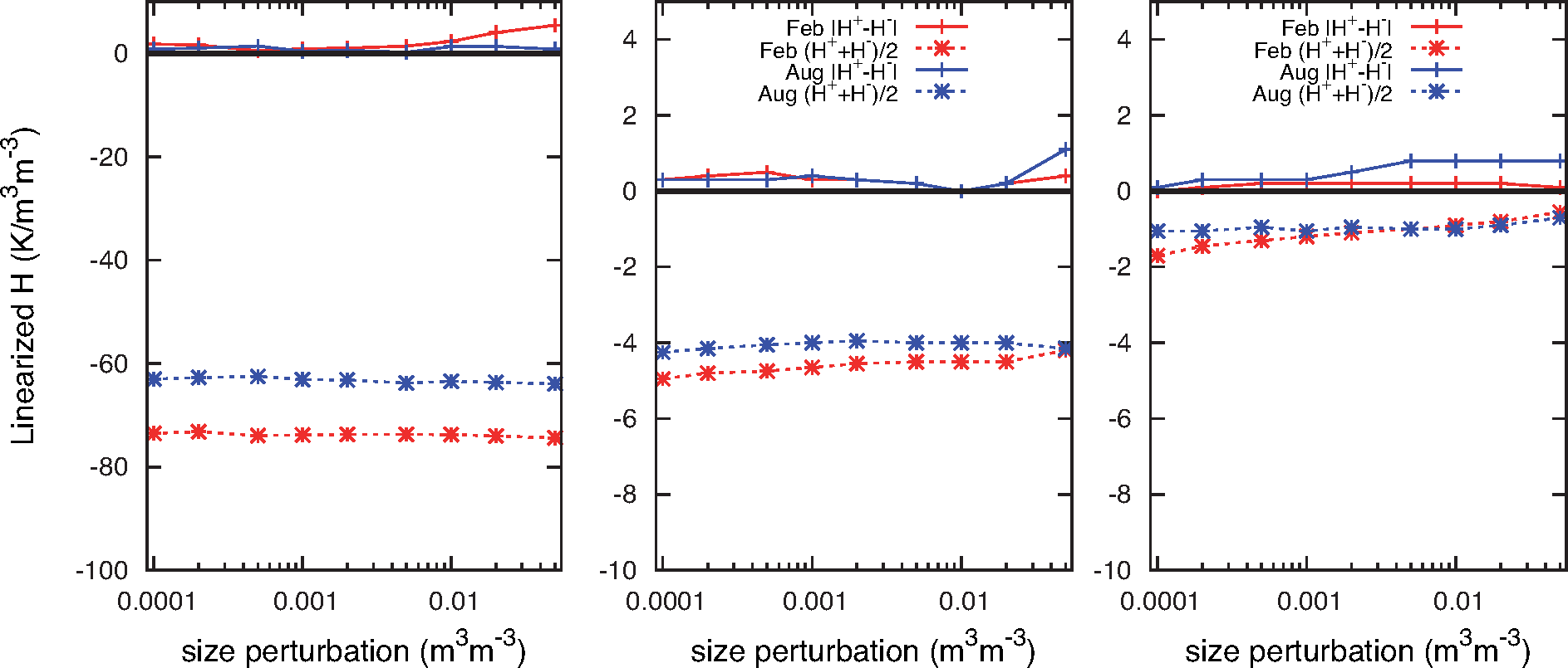
The size of the perturbation applied to the control vector to estimate the Jacobian components of screen-level variables was optimized by [22,39]. Here and for the sake of consistency, the same method was employed and extended to calibrate the SMOS components of the Jacobians. This is also the same method used in other centers ([49,50]); in a well-behaved deterministic system the Jacobians should be independent of the sign of the perturbation, and the mean Jacobian evaluated through a positive and negative perturbation of soil moisture, independent of the size of the perturbation δx_k within the linearity limits. Several one-week assimilation experiments at T159 spatial resolution were run in order to investigate the previous two requirements. A total of 9 perturbations in the range from 0.0001 to 0.1 m³/m⁻³, positive and negative, were applied to the three layers of soil moisture and during two weeks, in August 2011 and February 2012, hence studying the potential influence of very different meteorological conditions in the Jacobians. To avoid the signature of snow or ice, snow and frozen masks, based on forecasted snow depth and 2 m temperature fields, were applied to observed SMOS T_B. Also, grid points showing unrealistic large sensitivity to soil moisture perturbations were filtered out. In total, six incidence angles from 10° to 60°, in steps of 10°, were assimilated in these experiments. The Jacobians were obtained for each experiment, and the global average value with positive and negative perturbations is shown in Figure 1, for the top three soil layers.

A much larger sensitivity is observed in the first soil layer, as might be expected given that the penetration depth of the L-band is just a few cm. Note that this sensitivity is several orders of magnitude larger than for screen temperature as shown in [43]. Therefore, a larger correction of the first soil layer due to SMOS observations is expected compared to screen-level variables. The sensitivity of model T_B to soil moisture is negative, so in general terms, increasing soil moisture will decrease T_B. Only under very specific circumstances will this not be the case. For the second and third soil layers, the observed sensitivity to perturbed soil moisture is much lower than for the top layer, which is a consequence of the loss of the satellite sensor sensitivity with depth. It is surprising that the global averaged Jacobians turn out to be larger for February than for August, the latter with much drier soil conditions. However, one should bear in mind that the number of grid points used to compute the average Jacobians is very different for the two months. In fact, in February the northern latitudes are filtered out as they are covered by snow. These latitudes show lower sensitivity to soil moisture due to wetter conditions, and in February they do not contribute to the total average, which explains this larger value. Figure 1 also shows, as required, the Jacobians to be independent of the size of the perturbation. Small absolute differences different from zero point towards some instabilities of the numerical radiative transfer model. Those perturbations comprised between 0:001 and 0.01 m³•m⁻³ result in lower absolute differences, and for the sake of consistency with screen-level variables, 0.01 m³•m⁻³ was selected as the perturbation for the SMOS components of the Jacobians of the observation operator.

3. Experimental Validation

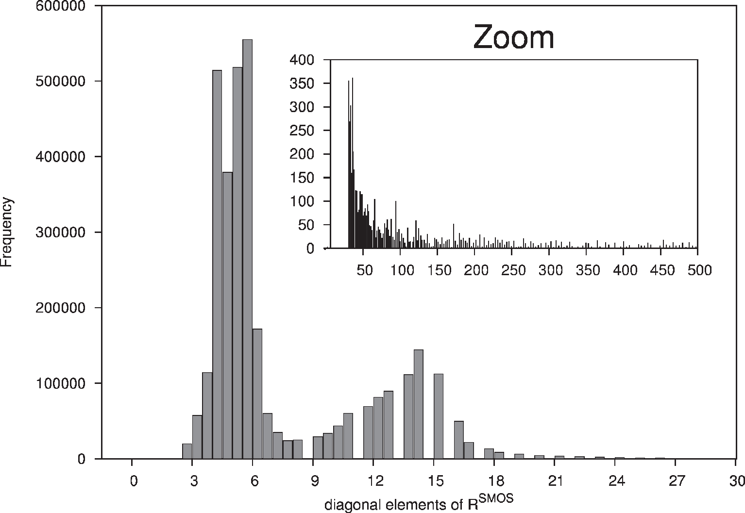
The approach explained above to assimilate SMOS T_B was implemented in the ECMWF SEKF and validated through two simple experiments in the coupled ECMWF land-atmospheric model: (a) a control run, consisting of assimilating only 2 m temperatures and 2 m relative humidity, as in the operational system (hereafter CTRL); (b) an experimental run, where SMOS T_B were assimilated in addition to screen-level variables, at 2 incidence angles (40° and 50°) with a margin of 0.5° (this means that for example, for 40° all observations with incidence angles between 39.5° and 40.5° will be considered), and the two pure polarisation modes (XX, YY) (hereafter denoted as EXPT). The period of the experiment spanned from 1 to 15 July 2012. The background and observation covariance error matrices are those explained in Section 2.3. Figure 2 shows the histogram of the diagonal element values of R^SMOS, representing the variance of the radiometric accuracy for 15 days of data filtered from snow and frozen soil. Most of them have low values, with a mean of 7.58 K², although observations with very large associated variance were also found, as shown in the zoom box in Figure 2. The analyses were carried out at global scale and at a spatial resolution of approximately 40 km to match the spatial resolution of SMOS observations and to avoid large horizontal correlations between SMOS observations. The upper-air analysis was constrained by using only conventional data and a few geostationary satellites, making both experiments computationally affordable. Increments were allowed to occur also in very dry regions with initial soil moisture lower than 0.01 m³•m⁻³. In these areas, SMOS observations can be very sensitive to any variation of the soil water content, and potentially it can bring a large benefit.

3.1. Bias Characterization and Correction

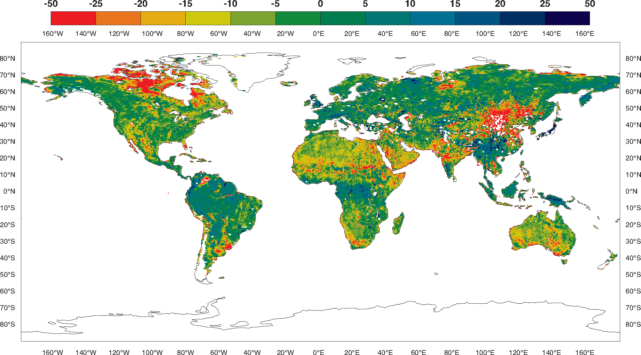
Using remote-sensing information to adjust model-based estimations in a land data assimilation system requires a certain degree of coherence between both sources of information. Bias between model and satellite data will unavoidably exist and successful merging of remote-sensing data and model data will rely on prior estimation and correction of these biases. In Figure 3 the averaged biases from 1 to 15 July 2012, at YY polarisation and 40°, between SMOS T_B and CMEM estimations are shown. Not only is a large average bias found (−8.29 K), but the biases have very uneven geographical distribution. Large negative biases are observed in northern Canada as well as in the wetlands. They are also large and negative in China, northern India and some regions of the Middle East, but in this case this is due to contamination by RFI.

Table 1. Mean bias and bias standard deviation (STD) between SMOS T_B and CMEM estimations for the period 1 to 15 July 2012.

	40XX	40YY	50XX	50YY
Mean Bias (K)	2.43	−8.29	−5.48	−5.74
STD (K)	15.53	14.72	18.51	14.21

shows the averaged bias and its standard deviation per incidence angle and polarisation. It shows that they can be also very different depending on the viewing angle and polarisation. The RTM estimations are on average slightly underestimated only at 40° and XX polarisation. Larger variability is observed in XX than in YY polarisation, as XX polarisation is more sensitive to soil moisture. These results are consistent with those observed on a dedicated ECMWF website for monitoring SMOS T_B: http://www.ecmwf.int/products/forecasts/d/charts/monitoring/satellite/smos/.

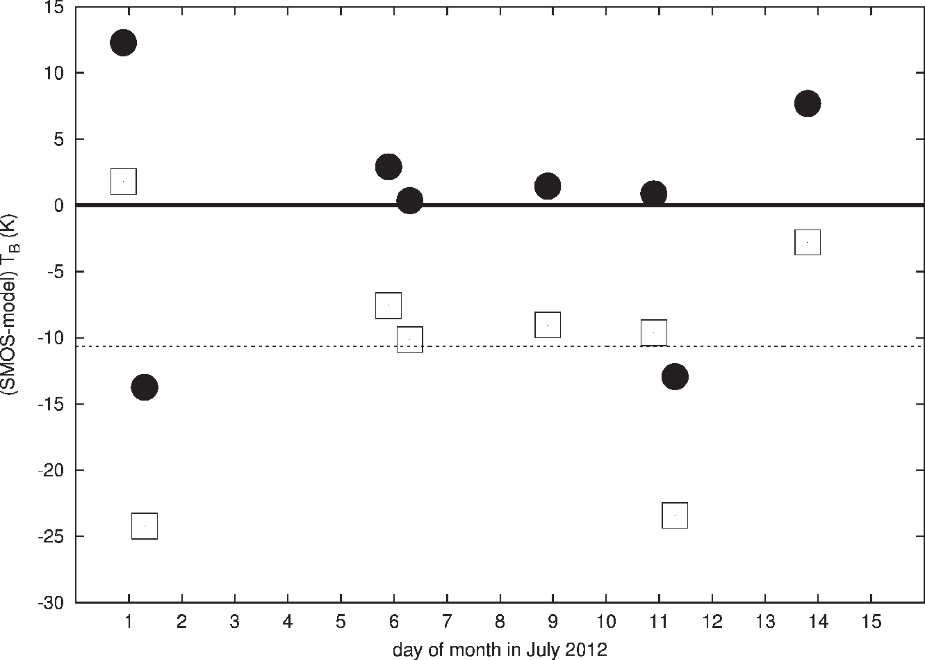
The method used here to rescale SMOS T_B to the RTM dynamical range is simple; the mean bias for the period under study was computed individually for each grid point, incidence angle and polarisation and then subtracted from each corresponding observation. This is just an approximation to more complex statistically based correction approaches, such as cumulative distribution matching [51] or least-squares regression techniques [52]. Since the correction is constant for each grid point, this method works efficiently in areas showing stable bias during the duration of the experiment, whereas substantial residual biases remain in grid points showing a large dynamic range of T_B. Figure 4 shows an example of the bias for a location in central Australia, before (squares) and after (filled dots) correction of the observations. While by construction, the averaged bias (after a correction of −10.39 K) is zero, the first and last observations along the studied period increase the bias. However, averaged at global scale the consistency between the rescaled observations and the model equivalents is higher, as the averaged rescaled T_B increases from 255.76 K to 259.91 K, which is more in agreement with the average of the simulated T_B, 259.12 K.

3.2. Quality Control

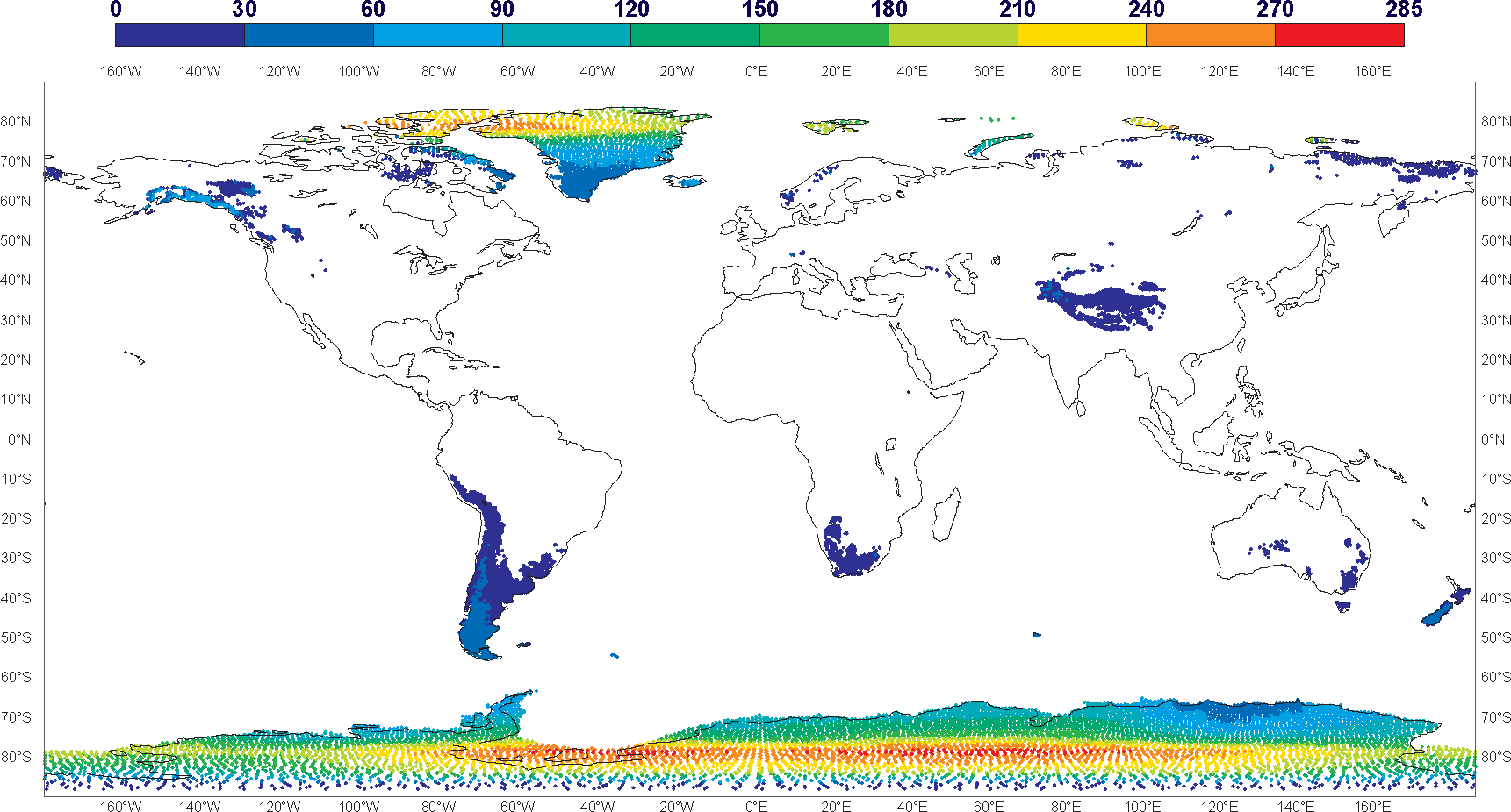
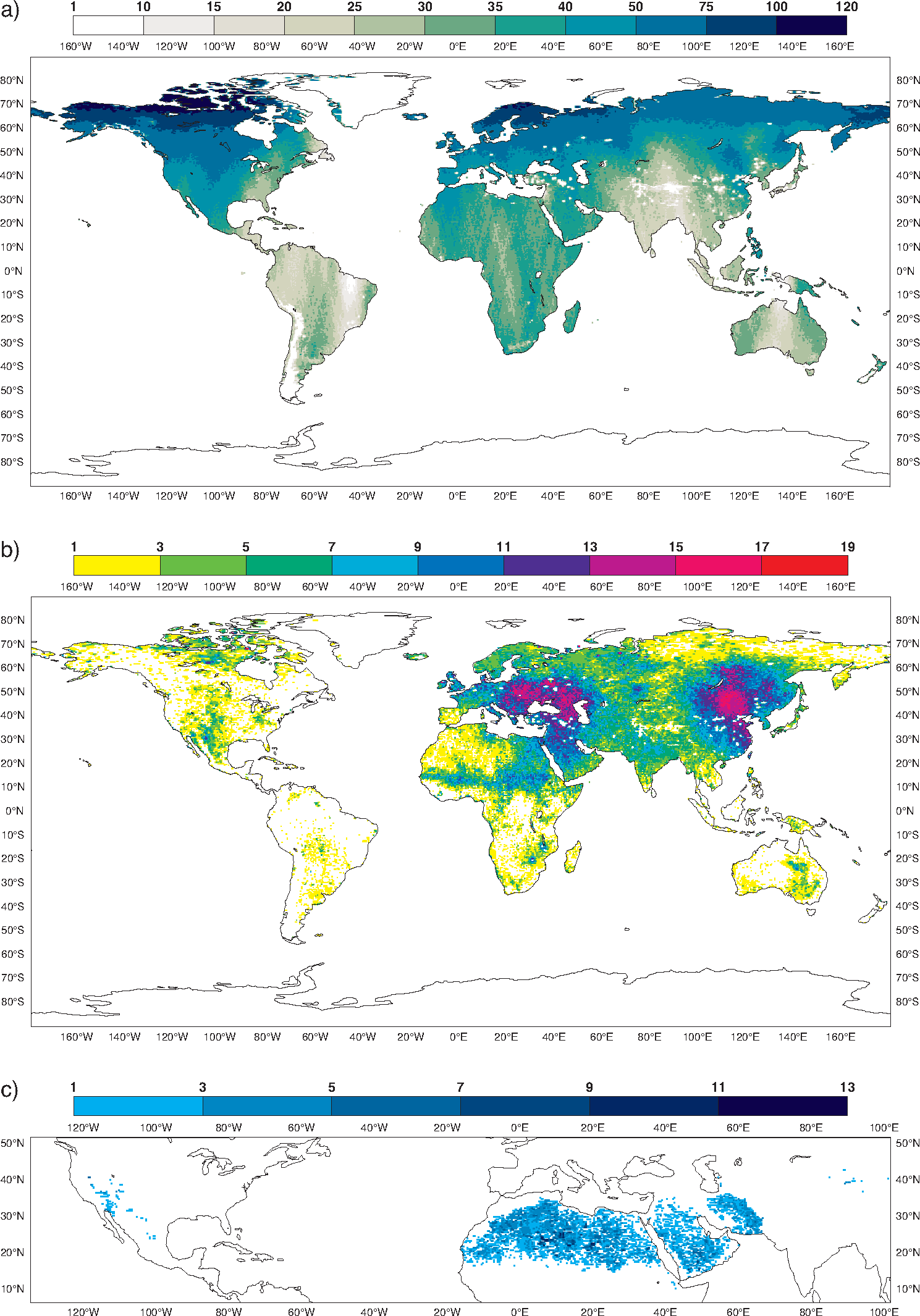
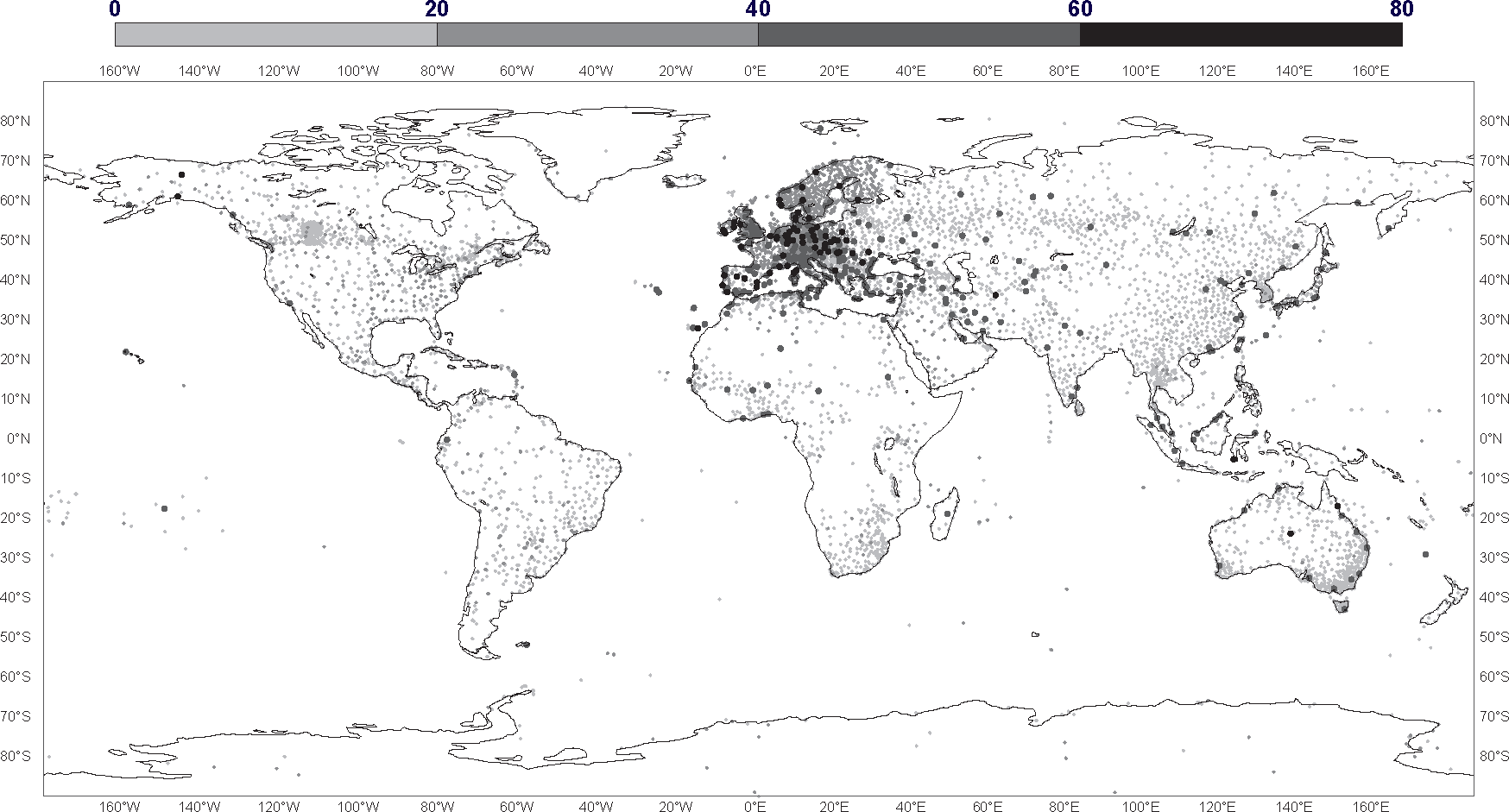
All the observations within the assimilation system are subjected to different quality checks, as a series of basic checks as described in [38], a snow mask and a RFI filter based on the NRT product flags, preventing spurious observations that are not consistent with the model being assimilated. The blank spaces in Figure 3 correspond to RFI filtered data. Figure 5a shows the number of SMOS observations available for assimilation within the SEKF in experiment EXPT. As expected the number increases with latitude, as the revisit time is shorter at higher latitudes. It also shows areas that have less frequent revisit satellite passes during the period of the experiment. However, the reduced number of available observations in the Himalayas and the Andes is due to previous filtering steps based on snow and frozen soils, as shown in Figure 6. The number of screen-level observations is the same in both experiments; they are especially dense in Europe but good coverage is also found in eastern and northern parts of the US, the east of Australia, China and South Africa, as shown in Figure 7. Further, each observation is compared to the model equivalent and a maximum acceptable difference is defined, which is called the first-guess check. For SMOS T_B this value is set to 20 K, based on the standard deviation of the SMOS T_B innovations. Figure 5b shows the number of observations rejected per grid point showing discrepancies larger than 20 K with the model simulation. There are two areas with a large number of rejections in Eurasia, the Middle East and China. This is due to RFI contamination. For the rest of the globe, very few observations are rejected. It is not known if the first-guess rejections are due to noisy observations or a deficient simulation. Very few screen-level observations are rejected by the first guess (limits are 5 K for T_2m and 20% for RH_2m). Simulated observations showing too large sensitivity to small perturbations of soil moisture are also rejected. Figure 5c shows the number of observations rejected by this check and their geographical distribution. They occur mainly in desert areas of North Africa and the Middle East, where due to the strong radiative heating, the surface temperature and soil effective temperature are very close, producing very large sensitivity of T_B to soil moisture variations, following the model of [53]. This effect is discussed in detail in [54].

3.3. Soil Moisture Increments

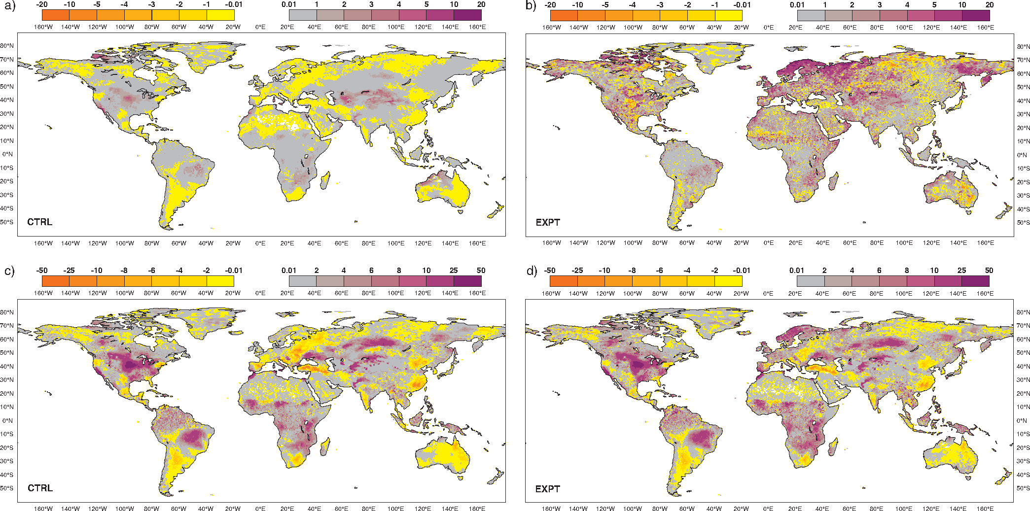
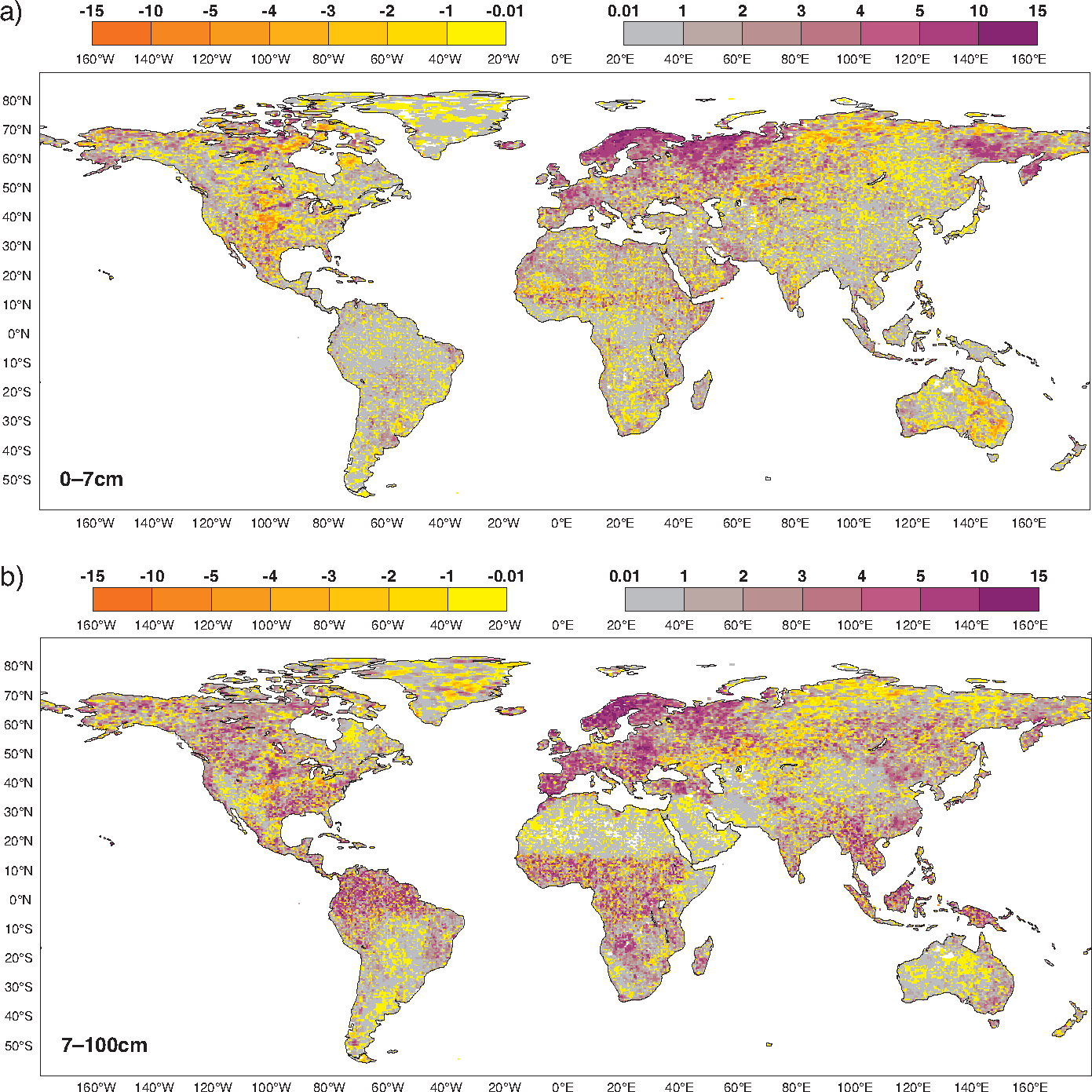
The total soil moisture increments for CTRL and EXPT experiments are shown in Figure 8 for the top 7 cm (which SMOS observations are sensitive to) and for the deep layer, which in this study is defined as the combination of the second and third model layers (7–100 cm, where SMOS observations have no or very little sensitivity). Analysis increments are mostly small for the top soil layer, below 1 mm if only T_2m and RH_2m observations are assimilated. Larger positive increments are observed in the Great Plains of the US, the western part of north Canada, central Asia and the northwestern part of Australia. Prior to use in the SEKF, screen-level variables are spatialised by an OI analysis scheme, which produces large spatialised patches of positive and negative increments. These increments will be more effective in areas where the SYNOP network is denser, as in Europe or the east of the US. Adding SMOS T_B to the observation vector has a significant impact on the increments of the top layer. Indeed, negative increments are now also observed in central US, northern Canada, Sahel, Siberia and eastern Australia, areas which according to SMOS observations are too wet. Contrarily, strong positive increments are added in western and northern Europe and fareeastern Russia. Increment patterns of the deeper layer are very similar for CTRL and EXPT, since the sensitivity of screen-level variables and remote-sensing data to soil moisture decreases with the soil depth. In fact, the information carried in the observations is propagated in the vertical dimension through the computation of dynamical Jacobians. The main difference in the increments of the deep layer is observed in west and north of Europe, for which SMOS data added water up to 10 mm.

Table 2. Total soil moisture increments (MInc) and their absolute values (MAInc) and standard deviation (STD), averaged at global scale, for CTRL and EXPT experiments. All values are in mm units.

	Surface Soil Layer (0–7 cm)			Deep Layer (7–100 cm)
	MInc	MAInc	STD	MInc	MAInc	STD
CTRL	0.13	0.18	0.62	0.66	2.50	3.88
EXPT	0.04	1.42	2.15	0.85	2.73	4.05

shows the global average of the soil moisture increments, as well as their absolute value and standard deviation, for the top and deep layer. It is observed that averaged at global scale, the net effect of assimilating SMOS data too is adding slightly less water to the top layer (0.04 mm) than assimilating only screen variables (0.13 mm), whereas it adds more water for the root zone (0.85 mm). Either for CTRL or EXPT, the absolute increments (global averaged) are larger for the deep layer. However, this is relative to the depth of each layer (70 mm for the top layer and 930 mm for the deep layer), and this turns into relative increments of the same order for both layers for CTRL, whereas for EXPT they are 7 times larger for the top layer compared to the deep layer. In the top soil layer, the variability of the increments with SMOS data are 3.5 times larger than if no SMOS data were assimilated. This means that EXPT is more dynamic at adjusting the top soil moisture than CTRL.

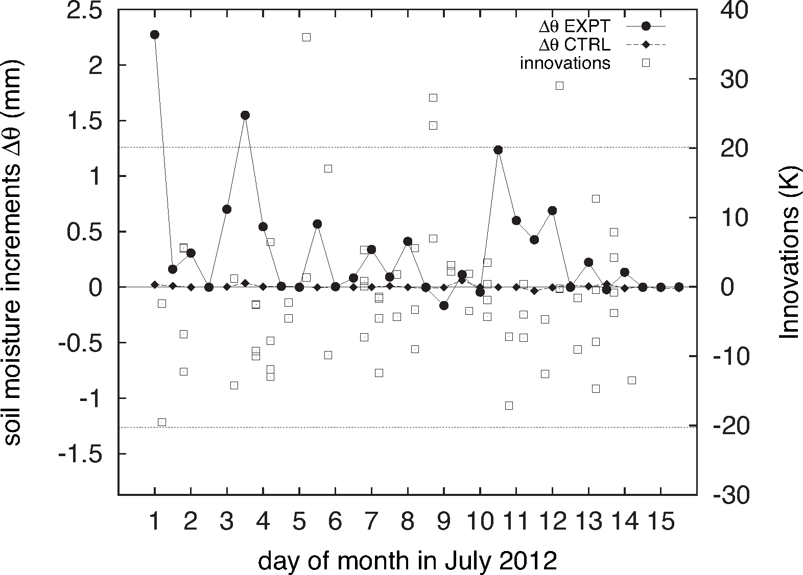
The differences in the accumulated increments between EXPT and CTRL are shown in Figure 9. The main difference in the top layer is observed in the north of Europe, which is seen wetter by SMOS data than the model prediction. A deeper investigation was carried out over a location in Sweden, where the assimilation of screen variables and SMOS data brings accumulated increments larger than 10 mm: Figure 10 shows that increments of the top layer are systematically positive with a value over 2 mm for the first analysis step. In contrast, increments are comparatively negligible if only T_2m and RH_2m observations are assimilated, despite being an area with a good density of SYNOP stations. The first large positive increment in Figure 10 is due to the combination of a large dry initial bias (produced by a simulated T_B that is too warm) and negative Jacobian values at this location (decreasing simulated T_B with a positive perturbation of soil moisture). Although the bias is large, it is not large enough to have data rejected by the first-guess check (threshold of −20 K). Most of the innovations in Figure 10 are negative and relatively large, which produces large total positive increments. Apart from being in an RFI influence area (see Figure 5), this is a challenging region for the RTM and the filtering system. Firstly because there are still observations under freezing conditions in July and secondly because this is a region with a large density of small lakes which are not yet resolved by the model. Therefore many of these pixels are interpreted as being completely covered by land with higher emissivity properties. This example shows the limitations of the simple bias correction approach adopted in EXPT. It is not efficient in pixels showing large variability of T_B, because significant biases are still present within the assimilation system. There is also a need to account for higher resolution information of the soil cover. This is likely the case too with other positive increments found at northern latitudes. However, interesting drying signatures are observed in semi-arid regions, as in the Great Plains of the US, the subsahelian region and the east of Australia, regions characterized by a low density of the vegetation canopy and large proportion of bare soil, thus where the SMOS signal contains very useful information about soil moisture.

3.4. Soil Moisture Analysis Behaviour

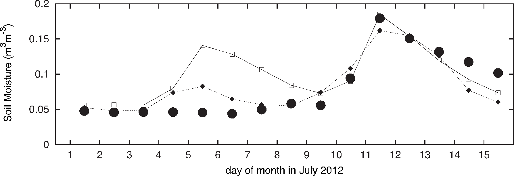
The behaviour of the assimilation system was validated in an area where the assimilation of SMOS showed more impact in this case study. The top 5 cm of the hourly soil moisture observations from five different stations located along a horizontal transect of 149 km between the states of Texas and New Mexico in the US, were retrieved and compared to the closest CTRL and EXPT analyses of the model top layer. The station names are, from west to east, Willow Wells, Crossroads, Lehman, Levelland and Reese Center and are part of the Soil Climate Analysis Network (SCAN). For this period of the year, the soil is very dry in this area and the remote-sensed T_B have good sensitivity to any variation in soil moisture. Only significant correlation values (based on the p-value test at 95% significant level) between in-situ observations and the CTRL and EXPT analyses were obtained for the Crossroads and Lehman stations. These stations are separated by a distance of 47.7 km. To minimize the local discrepancies that could be originated by comparing point-scale observations to analyses representative of a larger area, only averaged observations of the previous two stations were compared to the corresponding averaged soil moisture analyses of CTRL and EXPT. Figure 11 shows the daily mean in-situ observations and the daily mean analyses of CTRL and EXPT. From the first analysis, EXPT becomes drier than CTRL and closer to the observations. The averaged analysis of CTRL is very wet by day 5 of the experiment, as a response to a model precipitation, which is partially corrected by SMOS observations. Both experiments are able to reproduce the peak of moisture observed the 11 of July, whereas after that, EXPT dries slightly more than CTRL. On average over these two stations, EXPT obtains better coefficient of correlation (0.79) than CTRL (0.72), as well as lower RSMD (0.034 vs. 0.044 m³•m⁻³). Even if the system does not benefit yet from complete calibration, this exercise shows the potential of using remote-sensing data in areas where such data is expected to be very sensitive to soil moisture.

3.5. 2 m Temperature Impact

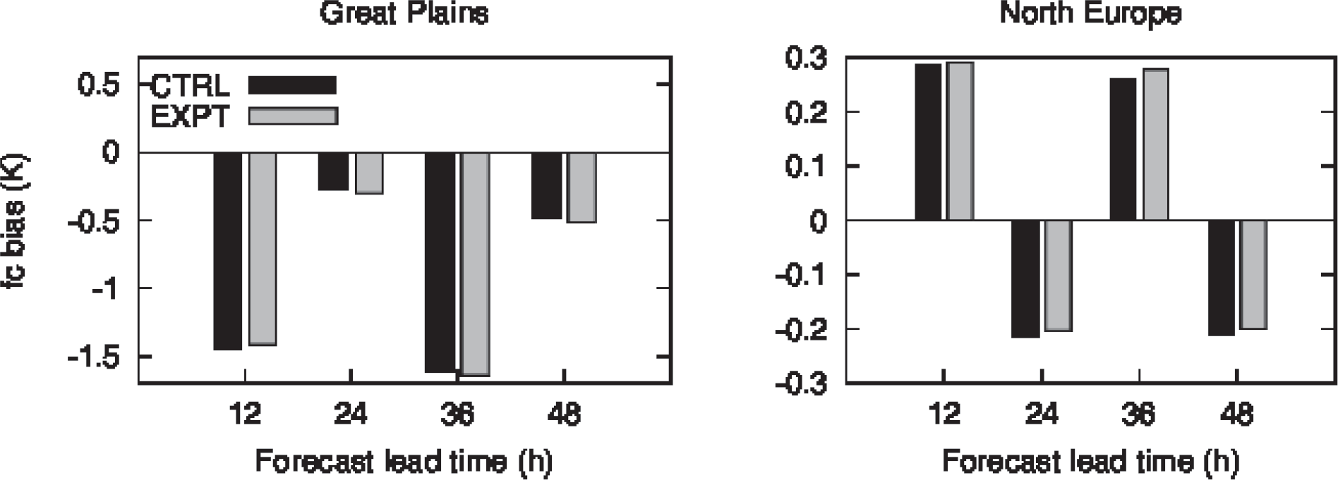
Figure 9 shows two regions where the impact of assimilating SMOS data was larger in terms of soil moisture: central US, where up to 15 mm of water was removed from the soil at certain locations, and the northern part of Europe, where on the other hand, up to 15 mm of water was added to the soil. The effect on the forecasts of T_2m for these two regions (central part of the Great Plains (coordinates: [N = 50, W = −110, S = 33, E = −93]), and the northern region of Europe (coordinates: [N = 75, W = 0, S = 52, E = 60])) is analysed in this section. Figure 12 shows the bias, defined as (observation-forecast), and RMS forecast error for four synoptic times (12 h, 24 h, 36 h and 48 h). Forecasts were initialised at 00UTC and compared with observations from all available SYNOP stations (see Figure 7) and averaged within these two regions. Note that not all in-situ SYNOP observations used in Figure 12 were assimilated due to quality control checks. A strong cycle of day-night bias is observed in both regions, but the amplitude is larger in central US with warm bias all day, much stronger in the early morning, as the model has more difficulties in accurately modeling temperature in stable conditions with strong temperature gradients close to the surface. Biases are reduced at mid-evening with less coupling between land and the near-surface atmosphere. The warm bias in the early morning at the Great Plains would be reduced by drying the air as it would allow the model temperature to get colder. In this sense, the negative soil moisture increments introduced by also assimilating SMOS data are consistent. However, the forecast biases of EXPT (with SMOS data) are slightly decreased at 12 h forecast compared to CTRL (without SMOS data), and slightly increased at longer forecast lead times. This means that the biases in air temperature do not necessarily come only from soil moisture inaccuracies, but are also originated by other sources, such as model errors. In the north of Europe the model has a cold bias during daytime and warm bias at nightime. The coupling in this region between land and atmosphere is weaker than in central US and forecast biases are smaller. Even if a substantial amount of water is added in this region by assimilating SMOS data, very little impact on 2 m temperature is observed. The RMS forecast error increases with the lead time (not shown) and is larger for the Great Plains domain (2.37 K for the Great Plains vs. 1.39 K for North Europe at 24 h forecast). This is due to the larger warmer bias early in the morning. However, the total effect of introducing SMOS and averaged over the four synoptic times (by averaging 60 forecasts, 15 for each lead time) is small. The impact on the 2 m dew point, from which the relative humidity can be derived, was also small (not shown).

4. Discussion

This paper presents an updated version of the soil moisture analysis in the ECMWF land-atmospheric coupled model. In contrast to most studies found in the literature with passive microwaves, the system presented in this paper makes it possible to assimilate direct information about soil moisture from passive microwave T_B to correct a model estimation. This is a new functionality of the ECMWF LDAS. As previously stated in this paper, the observation error information and the latency are two powerful reasons to assimilate direct radiances for soil moisture. Indeed, NWP centers are very constrained by time and require NRT access to observations. The SMOS data used in this study are available for use in the assimilation system between 3 and 4 h after sensing time (which makes their implementation possible in an operational context), whereas the SMOS level-2 soil moisture product is not available before 8 h, frequently beyond 12 h. However, one may wonder why the vast majority of assimilation studies for soil moisture analysis are based on satellite retrievals. A combination of several factors may explain it. A considerable reason is the complexity of the observation operator. In the case of soil moisture retrievals it becomes simple, frequently the identity matrix or a simple spatial interpolation, which makes the implementation in offline systems straightforward rather than needing an external interface with a full non-linear radiative transfer model. Additionally, the computational expense of assimilating satellite retrievals can be considerably lower. Other possible reasons can be less complex related tangent linear and adjoint operators, although in this paper the explicit computation of these operators is circumvented by approximating the Jacobian matrix by finite differences. For NRT applications, such as NWP, making the land system ready to assimilate NRT radiances is a key development, as integrating microwave T_B (as in SMOS data) in an operational structure can influence weather forecasts.

In Figure 3 large biases were found between SMOS observations and the CMEM equivalents, mainly due to RFI, topography and also for model grid cells (approximately 40 km in this study) with a significant portion covered by water bodies. RFI sources are strong in some regions of the Middle East and Asia, especially in China. To filter RFI-contaminated observations, the system presented in this paper relies partly on flags contained in the current version of the NRT processor (v5.05). These flags are succesful at pointing towards the main sources but not at the tails, which can be very important too. However, the first-guess check, as defined in Section 3.2, is effective at removing many other observations contaminated by RFI. The next operational version of the processor will account for a much improved algorithm of RFI detection. Concerning topography, the topographic effect in the L-band signal is not yet well resolved, and areas with strong orography can be easily underestimated by the RTM, as it occurs over the Alps region. Observations over these areas should be avoided until models are able to simulate their emission with reasonable accuracy. A possible recommended way to avoid these observations being assimilated is by using an external map of orographic slope. Large negative biases were also found in wetlands and over some wide rivers, such as the Amazon river (see Figure 3); the reason for this is that in the current operational land-surface model, if the portion of water within a model grid cell is lower than 50%, then the physical temperature of the soil within that cell will be used as input for the observation operator, ignoring the different temperature of the water body. In terms of T_B, this can turn into a much warmer simulation compared to the observation, which explains the negative bias found in the Amazon river. Reducing all these biases between the model and SMOS observations prior to assimilation is crucial. The analysis solution of the SEKF is based, among others, on the assumption that the assimilation system is free from bias. In this paper the observations were corrected to be more consistent with the model statistics. The methodology employed is simple and was based on subtracting the mean systematic bias from the observations, in a pointwise fashion. Although it preserves zero mean bias during the assimilation period, it does not account for day to day variability, and therefore it is limited with respect to the efficiency at removing bias in pixels showing large variability of T_B. An accurate evaluation of the impact of SMOS observations in the coupled forecasting system will have to account for more sophisticated bias correction methods, accounting at least for the differences between the mean and variance of both model and observations. But it is likely that even after bias correction, remaining bias will stay in the system. For instance, [36] reported large bias between SMOS observations and model equivalents from the microwave tau-omega radiative transfer model (which is a version of the CMEM RTM used in this study) before parameter calibration. But even after calibration, seasonal residual biases between −10 K and 10 K were remaining.

One of the main advantages of assimilating direct satellite measurements instead of satellite retrievals is that the observation error introduced in the assimilation system is better controlled. The values shown in Figure 2 are directly supplied by the data provider and represent an objective error representative of the observation. However, these values are likely underestimated if one takes into account that the observation error is also affected by other factors such as the sampling depth or the T_B algorithm reconstruction. In the present form, the weight given to SMOS observations in the analysis increment is likely to be overestimated and future experiments will have to account for other sources of error. The histogram of variances in Figure 2 showed a bimodal distribution. This reflects the particular geometry of the heterogeneous distribution of sensitivities within the field of view of SMOS observations. Pixels which are close to the boresight have better radiometric sensitivity (around [2.5–3] K) than those close to the edge of the field of view around [4–5.5] K, because the gain of the antenna decreases with the distance to the boresight.

The assimilation case study of Section 3 showed, for CTRL (representing a simplified configuration of the operational system,) similar relative soil moisture increments of the top layer (0–7 cm) and the deep layer (7–100 cm). As shown in Figure 8, screen-level variables produce very small corrections of soil moisture due to the low sensitivity to soil moisture variations and the small weight given in the assimilation system compared to the background value. This can be verified by projecting the background error matrix into observation space (assuming the values given in [22] for the T_2m and RH_2m Jacobian components) and comparing it to the variance of the observation errors. In contrast, EXPT assimilating also SMOS T_B, obtained relative increments up to 7 times larger for the top layer compared to the deep layer. This result means that the information contained in the SMOS observations impacts greatly on the first few cm of the soil, as would be expected from a type of observation that is very informative about the model top layer. Indeed, SMOS strongly contributes to the top increments, being nearly 8 times larger in absolute values for EXPT than for CTRL. Despite all the future necessary adjustments of the assimilation system, this is a very encouraging result to make use of direct information from remote-sensing data to effectively adjust the state of the soil. On the other hand, the impact in the deep layer is small, just 1.1 times larger for EXPT than for CTRL, but this was expected due to the rapid decrease in sensitivity with depth. The large increments observed at depth in northern and western Europe are likely due to the combined effect of RFI and residual biases that were assimilated (as the simple bias correction method used does not account for day to day variability), but also to the frequent amount of water bodies found in northern Europe and currently unresolved by the land-surface model. Several adjustments will be necessary to make sure that the top layer information is propagated consistently through the vertical profile. The accumulated impact of SMOS assimilation on the top soil layer over time should eventually have a larger impact in the deeper layers. This could be observed after long periods (months to years), for example through adjustments of infiltration from the shallow layer into the deeper layers.

The experiment of this paper compared soil moisture analyses (obtained with SMOS data) with averaged point-scale observations in a dry area showing strong increments. Although more dedicated strategies could be used to validate the analysis (for example by upscaling the available in-situ data to the coarser satellite footprint scale [55]), and the number of in-situ samples used in this paper is not sufficient to conclude positive impact, there is a potential benefit with deserves to be investigated over longer periods and with larger number of observations. The experiment using SMOS data also showed neutral impact on air temperature. But even neutral impact is beneficial to complement the existing data, as the whole system can benefit from the availability of one source of data if the other is unavailable. The neutral impact on air temperature points also towards possible deficiencies in the coupled system, although it cannot provide an answer for their origin. For example, the large response of soil moisture to SMOS data in the Great Plains of the US was not followed by a significant impact on 2 m temperature, likely due to other factors, such as an inaccurate radiative forcing or inadequate evaporation formulation. If NWP centers aim at benefiting from the new wealth of remote-sensing data providing direct observations of soil moisture, they will likely have to cope with land-atmospheric coupling issues to make the behaviour of all the Earth-system components consistent with the new data.

5. Conclusions and Perspectives

This paper presents a new version of the ECMWF LDAS. The good behaviour of the new system was validated by comparing the analyses of a 15-day global-scale experiment using an operational configuration with a similar one but adding SMOS T_B. This is a necessary and logical step in the process of implementating the operational assimilation of new data sensitive to soil moisture. The results presented in this study highlight the potential benefits of the new data. This paper indicates that the assimilation of SMOS data impacts strongly on the top soil layer, up to seven times more than only the use of indirect information from screen data. This result is very encouraging, especially where soil moisture evolves without any observational constrain due to the unavailability or low density of screen variables. Nonetheless, the impact in the shallow layer will likely be reduced by using a larger, more realistic error representative of the observations. The impact in the root-zone is moderate for the 15-days period of the experiment in this study, and comparable to the net volume of water adjusted by screen-level variables. However, the deep layer still benefits from assimilation, as the SEKF used in this study is able, to some extent, to propagate the soil moisture information into deeper layers throughout the Jacobian computation. The assimilation of SMOS T_B does not have an homogeneous impact over land surfaces. Large increments were obtained in dry areas and characterized by low vegetation density, where SMOS has a lot of potential. But also large increments were found in areas with numerous water bodies, not resolved yet by the land-surface model. These results should be taken with caution and are only indicative of the potential benefits of using direct passive microwave radiances for soil moisture estimation. The real benefits of using SMOS data in this system will only be duly evaluated if longer-term assimilation experiments are investigated, spanning at least a boreal summer or a whole hydrological year. This should be accompanied by an exhaustive validation against all available in-situ soil moisture data and atmospheric observations.

The efficiency of assimilating SMOS T_B in the ECMWF LDAS will be enhanced by future model and data assimilation developments. Soon, the introduction of a model providing resolved temperatures for inland water bodies will provide more accurate inputs for the RTM where significant portions of a model grid cell are covered by water. Other future model developments include a more accurate description of the daily cycle of convective precipitation, therefore reducing the uncertainty of the atmospheric forcing, or the introduction of soil temperature in the SEKF, which will enhance the advantages of assimilating direct T_B instead of satellite retrievals. Regarding the assimilation system, more sophisticated bias correction schemes are necessary and are currently being implemented to guarantee that only random differences between model estimations and the observations are corrected. In addition, other developments include a simple scheme to reduce the noise of the assimilated SMOS observations [56] and a detailed calibration of each element of the assimilation system. For example, the correct weight given to the assimilated observations in the SEKF as well as to the model error are being investigated. All these developments will make it possible to optimize the use of SMOS T_B in the ECMWF LDAS.

References

- Viterbo, P. The Representation of Surface Processes in General Circulation Models. Ph.D. Thesis, University of Lisbon, Lisbon, Portugal, 1996. [Google Scholar]
- Beljaars, A.C.M.; Viterbo, P.; Miller, M. The anomalous rainfall over the United States during July 1993: Sensitivity to land surface parameterization and soil moisture anomalies. J. Hydrometeorol. 1996, 124, 362–383. [Google Scholar]
- Douville, H.; Viterbo, P.; Mahfouf, J.; Beljaars, A. Evaluation of optimal interpolation and nudging techniques for soil moisture analysis using FIFE data. Am. Meteorol. Soc. 2000, 128, 1733–1756. [Google Scholar]
- Mahfouf, J.F.; Viterbo, P.; Douville, H.; Beljaars, A.; Saarinen, S. A Revised Land Surface Analysis Scheme in the Integrated Forecasting System; Technical Report 88; European Centre for Medium-Range Weather Forecasts: Reading, UK, 2000. [Google Scholar]
- Drusch, M.; Viterbo, P. Assimilation of screen-level variables in ECMWF’s Integrated Forecast System: A study on the impact of the forecast quality and analyzed soil moisture. Am. Meteorol. Soc. 2007, 135, 300–314. [Google Scholar]
- Van-Den-Hurk, B.; Ettema, J.; Viterbo, P. Analysis of soil moisture changes in Europe during a single growing season in a new ECMWF soil moisture assimilation system. J. Hydrometeorol. 2008, 9, 116–131. [Google Scholar]
- Koster, R.D.; Dirmeyer, P.A.; Guo, Z.; Bonan, G.; Chan, E.; Cox, P.; Gordon, C.T.; Kanae, S.; Kowalczyk, E.; Lawrence, D.; et al. Regions of strong coupling between soil moisture and precipitation. Science 2004, 305, 1138–1140. [Google Scholar]
- Koster, R.; Yamada, T.J.; Balsamo, G.; Berg, A.; Boisserie, M.; Dirmeyer, P.; Doblas-Reyes, F.; Drewitt, G.; Gordon, C.; Guo, Z.; et al. The second phase of the global land-atmosphere coupling experiment: soil moisture contribution to subseasonal forecast skill. J. Hydrometeorol. 2011, 12, 805–822. [Google Scholar]
- Weisheimer, A.; Doblas-Reyes, P.; Jung, T.; Palmer, T. On the predictability of the extreme summer 2003 over Europe. Geophys. Res. Lett. 2011, 38. [Google Scholar] [CrossRef]
- Dirmayer, P. Using a global soil wetness dataset to improve seasonal climate simulation. J. Clim. 2000, 13, 2900–2921. [Google Scholar]
- Ni-Meister, W.; Walker, J.; Houser, P. Soil moisture initialization for climate prediction: Characterization of model and observation errors. J. Geophys. Res. 2005, 110. [Google Scholar] [CrossRef]
- Seneviratne, S.; Corti, T.; Davin, E.; Hirschi, M.; Jaeger, E.; Lehner, I.; Orlowsky, B.; Teuling, A.J. Investigating soil moisture-climate interactions in a changing climate: A review. Earth Sci. Rev. 2010, 99, 125–161. [Google Scholar]
- Delworth, T.; Manabe, S. The influence of potential evaporation on the variabilities of simulated soil wetness and climate. J. Clim. 1988, 1, 523–547. [Google Scholar]
- Delworth, T.; Manabe, S. The influence of soil wetness on near-surface atmospheric variability. J. Clim. 1989, 2, 1447–1462. [Google Scholar]
- Koster, R.; Suarez, M.J.; Heiser, M. Variance and predictability of precipitation at seasonal- to-interannual timescales. J. Hydrometeorol. 2000, 1, 26–46. [Google Scholar]
- Calvet, J.C.; Noilhan, J.; Bessemoulin, P. Retrieving the root-zone soil moisture from surface soil moisture or temperature estimates: A feasibility study based on field measurements. J. Appl. Meteorol. 1998, 37, 371–386. [Google Scholar]
- Muñoz-Sabater, J.; Jarlan, L.; Calvet, J.; Bouyssel, F.; de Rosnay, P. From near surface to root-zone soil moisture using different assimilation techniques. J. Hydrometeorol. 2007, 8, 194–206. [Google Scholar]
- Reichle, R.; Koster, R.D.; Liu, P.; Mahanama, S.P.P.; Njoku, E.G.; Owe, M. Comparison and assimilation of global soil moisture retrievals from the Advanced Microwave Scanning Radiometer for the Earth Observing System (AMSR-E) and the Scanning Multichannel Microwave Radiometer (SMMR). J. Geophys. Res. 2007, 112. [Google Scholar] [CrossRef]
- Draper, C.S.; Mahfouf, J.F.; Walker, J.P. Root zone soil moisture from the assimilation of screen-level variables and remotely sensed soil moisture. J. Geophys. Res. 2011, 116, D02127. [Google Scholar]
- Giard, D.; Bazile, E. Implementation of a new assimilation scheme for soil and surface variables in a global NWP model. Mon. Wea. Rev. 2000, 128, 997–1015. [Google Scholar]
- Belair, S.; Crevier, L.; Mailhot, J.; Bilodeau, B.; Delage, Y. Operational implementation of the ISBA land surface scheme in the Canadian regional weather forecast model. Part I: Warm season results. J. Hydrometeorol. 2003, 4, 352–370. [Google Scholar]
- Drusch, M.; de Rosnay, P.; Balsamo, G.; Andersson, E.; Bougeault, P.; Viterbo, P. Towards a Kalman filter based soil moisture analysis system for the operational ECMWF Integrated Forecast System. Geophys. Res. Lett. 2009, 36. [Google Scholar] [CrossRef]
- De Rosnay, P.; Balsamo, G.; Albergel, C.; Muñoz-Sabater, J.; Isaksen, L. Initialisation of land surface variables for Numerical Weather Prediction. Surv. Geophys. 2012. [Google Scholar] [CrossRef]
- Draper, C.S.; Mahfouf, J.F.; Walker, J.P. An EKF assimilation of AMSR-E soil moisture into the ISBA land surface scheme. J. Geophys. Res. 2009, 114, D20104. [Google Scholar]
- Kerr, Y.; Waldteufel, P.; Wigneron, J.P.; Delwart, S.; Cabot, F.; Boutin, J.; Escorihuela, M.; Font, J.; Reul, N.; Gruhier, C.; et al. The SMOS mission: New tool for monitoring key elements of the Global Water Cycle. IEEE Proc. 2010, 98, 666–687. [Google Scholar]
- Kerr, Y.; Font, J.; Martin-Neira, M.; Mecklenburg, S. Introduction to the special issue on the ESA’s Soil Moisture and Ocean Salinity Mission (SMOS) instrument performance and first results. IEEE Trans. Geosci. Remote Sens. 2012, 50, 1351–1353. [Google Scholar]
- Lahoz, W.; de Lannoy, G. Closing the gaps in our knowledge of the hydrological cycle over land: Conceptual problems. Surv. Geophys. 2014, 35, 623–660. [Google Scholar]
- Reichle, R.; Crow, W.; Kepenne, C. An adaptive ensemble Kalman filter for soil moisture data assimilation. Water Resour. Res. 2008, 44. [Google Scholar] [CrossRef]
- Scipal, K.; Drusch, M.; Wagner, W. Assimilation of an ERS scatterometer-derived soil moisture index in the ECMWF numerical weather prediction system. Adv. Water Resour. 2008, 31, 1101–1112. [Google Scholar]
- Kumar, S.; Reichle, R.; Koster, R.D.; Crow, W.T.; Peters-Lidards, C. Role of Subsurface Physics in the Assimilation of Surface Soil Moisture Observations. J. Hydrometeorol. 2009, 10, 1534–1547. [Google Scholar]
- Mahfouf, J.F. Assimilation of satellite-derived soil moisture from ASCAT in a limited-area NWP model. Q. J. R. Meteorol. Soc. 2010, 136, 784–798. [Google Scholar]
- Draper, C.; Reichle, R.; de Lannoy, G.; Liu, Q. Assimilation of passive and active microwave soil moisture retrievals. Geophys. Res. Lett. 2012, 39. [Google Scholar] [CrossRef]
- Sahoo, A.; de Lannoy, G.; Reichle, R.; Houser, P. Assimilation and downscaling of satellite observed soil moisture over the Little River experimental watershed in Georgia, USA. Adv. Water Resour. 2013, 52, 19–33. [Google Scholar]
- Renzullo, L.; van Dijk, A.; Perraud, J.M.; Collins, D.; Henderson, B.; Jin, H.; Smith, A.; McJannet, D. Continental satellite soil moisture data assimilation improves root-zone moisture analysis for water resources assessment. J. Hydrometeorol. 2014, 519, 2742–2762. [Google Scholar]
- Seuffert, G.; Wilker, H.; Viterbo, P.; Mahfouf, J.; Drusch, M.; Calvet, J. Soil moisture analysis combining screen-level parameters and microwave brightness temperature: A test with field data. Geophys. Res. Lett. 2003, 30, 1498–1501. [Google Scholar]
- Lannoy, G.D.; Reichle, R.; Pauwels, V. Global calibration of the GEOS-5 L-band microwave radiative transfer model over Nonfrozen land using SMOS observations. J. Hydrometeorol. 2013, 14, 765–785. [Google Scholar]
- Montzka, C.; Grant, J.; Moradkhani, H.; Franssen, H.; Weihermller, L.; Drusch, M.; Vereecken, H. Estimation of radiative transfer parameters from L-band passive microwave brightness temperatures using advanced data assimilation. Vadose Zone J 2013, 12. [Google Scholar] [CrossRef]
- Muñoz-Sabater, J.; Fouilloux, A.; de Rosnay, P. Technical implementation of SMOS data in the ECMWF Integrated Forecasting System. IEEE Geosci. Remote Sens. Lett. 2012, 9, 252–256. [Google Scholar]
- Balsamo, G.; Bouyssel, F.; Noilhan, J. A simplified bi-dimensional variational analysis of soil moisture from screen-level observations in a mesoscale numerical weather-prediction model. Q. J. R. Meteorol. Soc. 2004, 130, 895–915. [Google Scholar]
- De Rosnay, P.; Drusch, M.; Vasiljevic, D.; Balsamo, G.; Albergel, C.; Isaksen, L. A Simplified Extended Kalman Filter for the global operational soil moisture analysis at ECMWF. Q. J. R. Meteorol. Soc. 2012, 139, 1199–1213. [Google Scholar]
- Haseler, J. Early Delivery Suite; Technical Report 454; European Centre for Medium-Range Weather Forecasts: Reading, UK, 2004. [Google Scholar]
- Balsamo, G.; Viterbo, P.; Beljaars, A.; van den Hurk, B.; Hirschi, M.; Betts, A.; Scipal, K. A revised hydrology for the ECMWF model: Verification from field site to terrestrial water storage and impact in the Integrated Forecast System. J. Hydrometeorol. 2009, 10, 623–643. [Google Scholar]
- Drusch, M.; Holmes, T.; de Rosnay, P.; Balsamo, G. Comparing ERA-40 based L-band brightness temperatures with Skylab observations: A calibration/validation study using the Community Microwave Emission Model. J. Hydrometeorol. 2009, 10, 213–226. [Google Scholar]
- De Rosnay, P.; Drusch, M.; Boone, A.; Balsamo, G.; Decharme, B.; Harris, P.; Kerr, Y.; Pellarin, T.; Polcher, J.; Wigneron, J.P. AMMA Land Surface Model intercomparison experiment coupled to the Community Microwave Emission Model: ALMIP-MEM. J. Geophys. Res. 2009, 114, D05108. [Google Scholar]
- Muñoz-Sabater, J.; de Rosnay, P.; Balsamo, G. Sensitivity of L-band NWP forward modelling to soil roughness. Int. J. Remote Sens. 2011, 32, 5607–5620. [Google Scholar]
- De Rosnay, P.; Muñoz-Sabater, J.; Drusch, M.; Albergel, C.; Balsamo, G.; Boussetta, S.; Isaksen, L.; Thépaut, J. Bias correction for SMOS data assimilation in the ECMWF Numerical Weather Prediction System. P.C., Proceedings of the ESA Living Planet Symposium, Edinburgh, UK, 9–11 September 2013.
- Geer, A.; Bauer, P.; O’Dell, C. A revised cloud overlap scheme for fast microwave radiative transfer. J. Appl. Meteorol. 2009, 48, 2257–2270. [Google Scholar]
- Hess, R. Assimilation of screen level variables by variational soil moisture analysis. Meteorol. Atmos. Phys. 2001, 77, 145–154. [Google Scholar]
- Mahfouf, J.F.; Bergaoui, K.; Draper, C.; Bouyssel, F.; Taillefer, F.; Taseva, L. A comparison of two off-line soil analysis schemes for assimilation of screen level observations. J. Geophys. Res. 2009, 114, D08105. [Google Scholar]
- Dharssi, I.; Steinle, P.; Candy, B. Towards a Kalman Filter Based Land Surface Data Assimilation Scheme for Access; Technical Report No. 054; Centre for Australian Weather and Climate Research: Melbourne, Australia, 2012. [Google Scholar]
- Reichle, R.; Koster, R. Bias reduction in short records of satellite soil moisture. Geophys. Res. Lett. 2004, 31. [Google Scholar] [CrossRef]
- Crow, W. Continental-scale evaluation of remotely sensed soil moisture products. IEEE Geosci. Remote Sens. Lett. 2007, 4, 451–455. [Google Scholar]
- Wigneron, J.P.; Laguerre, L.; Kerr, Y. A simple parameterization of the L-band microwave emission from rough agricultural soils. IEEE Trans. Geosci. Remote Sens. 2001, 39, 1697–1707. [Google Scholar]
- Muñoz-Sabater, J.; de Rosnay, P.; Isaksen, L. Hot-Spot Analysis, PII-WP2300; Technical Report; European Centre for Medium-Range Weather Forecasts: Reading, UK, 2013. [Google Scholar]
- Crow, W.T.; Berg, A.A.; Cosh, M.H.; Loew, A.; Mohanty, B.P.; Panciera, R.; deRosnay, P.; Ryu, D.; Walker, J.P. Upscaling sparse ground-based soil moisture observations for the validation of coarse-resolution satellite soil moisture products. Rev. Geophys. 2012, 50. [Google Scholar] [CrossRef]
- Muñoz-Sabater, J.; de Rosnay, P.; Jiménez, C.; Isaksen, L. SMOS brightness temperatures angular noise: characterization, filtering and validation. IEEE Trans. Geosci. Remote Sens. 2014, 52, 5827–5839. [Google Scholar]