Article

Mapping of Agricultural Crops from Single High-Resolution Multispectral Images—Data-Driven Smoothing vs. Parcel-Based Smoothing

1
Department of Geodesy and Photogrammetry, Nevsehir H.B.V. University, 50300 Nevsehir, Turkey
2
Photogrammetry and Remote Sensing, ETH Zurich, 8093 Zurich, Switzerland
*
Author to whom correspondence should be addressed.
Remote Sens. 2015, 7(5), 5611-5638; https://doi.org/10.3390/rs70505611
Submission received: 23 February 2015 / Revised: 16 April 2015 / Accepted: 24 April 2015 / Published: 5 May 2015

Abstract

:
Mapping agricultural crops is an important application of remote sensing. However, in many cases it is based either on hyperspectral imagery or on multitemporal coverage, both of which are difficult to scale up to large-scale deployment at high spatial resolution. In the present paper, we evaluate the possibility of crop classification based on single images from very high-resolution (VHR) satellite sensors. The main objective of this work is to expose performance difference between state-of-the-art parcel-based smoothing and purely data-driven conditional random field (CRF) smoothing, which is yet unknown. To fulfill this objective, we perform extensive tests with four different classification methods (Support Vector Machines, Random Forest, Gaussian Mixtures, and Maximum Likelihood) to compute the pixel-wise data term; and we also test two different definitions of the pairwise smoothness term. We have performed a detailed evaluation on different multispectral VHR images (Ikonos, QuickBird, Kompsat-2). The main finding of this study is that pairwise CRF smoothing comes close to the state-of-the-art parcel-based method that requires parcel boundaries (average difference ≈ 2.5%). Our results indicate that a single multispectral (R, G, B, NIR) image is enough to reach satisfactory classification accuracy for six crop classes (corn, pasture, rice, sugar beet, wheat, and tomato) in Mediterranean climate. Overall, it appears that crop mapping using only one-shot VHR imagery taken at the right time may be a viable alternative, especially since high-resolution multitemporal or hyperspectral coverage as well as parcel boundaries are in practice often not available.

Graphical Abstract

1. Introduction

Monitoring agricultural lands and estimating crop production are crucial for countries whose economy heavily depends on agricultural commerce. This includes not only keeping track of the past production, but also short-term monitoring and yield estimation, to forecast agricultural production and inform marketing and trading decisions [1]. Traditionally up-to-date information of crop production is acquired by farmer declarations and/or ground visits of the fields. This procedure is not only subject to some errors and inconsistencies but also time consuming and expensive [2]. Hence, there is a demand for automated crop classification. However, the problem has not yet been solved completely; in particular for high resolutions at the level of individual fields (ground sampling distance in the range of 1–5 m), where coverage with dedicated sensors such as hyper-spectral cameras or polarimetric RADAR is prohibitively expensive.
A number of review papers have described the classification work carried out in the past and further elaborated on the advantages and disadvantages of the developed approaches, e.g., [3,4]. Here, we limit ourselves to supervised classification. In agreement with much of the literature (e.g., [4,5,6,7,8]) we prefer to start from labeled training examples of each class, since different crops may in some cases not exhibit the clear spectral separability required by unsupervised approaches [9]. In contrast to many other works, we prefer to use a single multispectral image for classification. Our motivation to use single-date imagery instead of multitemporal (or multisource) data is as follows: (i) single-date multispectral imagery is easier to obtain and cheaper; (ii) in productive crop fields, crop types can change on an almost monthly basis, which challenges multitemporal approaches and requires additional resources for frequent field work. In this study we therefore focus on the potential of (supervised) crop classification with single-date, high-resolution multispectral imagery.
The literature on crop classification is vast. In accordance with the topic of our investigation we only discuss supervised methods dealing with single-date optical images. Early efforts were dominated by pixel-based approaches, in which each pixel is separately categorized into one of the pre-determined classes, according to its spectral properties. In agricultural (and other) applications, the spectral properties are strongly influenced by changing imaging conditions, e.g., illumination, variations in soil moisture or nutrients, etc. Per-pixel classification methods often fail to capture the intra-class variability and therefore mislabel a rather large number of pixels. To increase robustness, it has been proposed to include additional grouping information rather than consider pixels in isolation. The basic idea of so-called parcel-based approaches is to divide the image into homogeneous regions using agricultural parcel boundaries, i.e., the location and extent of each field is assumed to be known a priori, e.g., [7,10,11,12,13]. Despite the success of the parcel-based approach, a drawback is that up-to-date parcel boundaries are not available for many agricultural areas, and collecting parcel or even field boundaries through interactive digitization and field observations is a time-consuming and expensive process. To bypass that effort object-based image analysis replaces the true field boundaries by the segment boundaries of an over-segmentation into homogeneous areas [14]. The segments are then labeled instead of the parcels, e.g., [15,16,17]. Such object-based image segmentation has gained quite some popularity, e.g., [2,18,19,20,21,22,23,24,25,26,27,28,29]. It often works well, but suffers from the conceptual problem that it aims to find segments made up of a single class during preprocessing, when by definition the class information is not yet available. As a consequence, the method tends to be sensitive to the (additional) parameters of the segmentation step, which directly affect the accuracy of the resulting thematic maps [25,30].
An alternative way to exploit information from larger pixel neighborhoods is to classify on a per-pixel level, but include a smoothness prior into the classification framework. The smoothness assumption corresponds to the basic fact that, as soon as the spatial sampling is dense enough, neighboring pixels tend to have the same class label. Schindler recently provided an overview and comparison of smooth labeling methods for land cover classification [31]. Both local filtering methods and global labeling solutions were investigated in the study. The most striking conclusion was the magnitude of the performance boost (up to 33%) after imposing the smoothness prior. The best performance was achieved using global conditional random field (CRF) labeling with graph cuts [32]. In spite of its popularity in image processing, to our knowledge, only a limited number of studies exist that use graph cuts in remote sensing image classification, predominantly in the context of hyperspectral images, e.g., [33,34,35,36,37,38]. In line with the image processing literature, they conclude that the CRF formulation improved the classification accuracy and call for further experimental evaluations.
In this paper, we investigate a general framework for crop classification in agricultural lands from high-resolution, single-date optical satellite images, based on the CRF formulation. Specifically, the main objective of this work is to expose the performance difference between state-of-the-art parcel-based smoothing and purely data-driven CRF smoothing, which has to our knowledge not yet been investigated in the literature. Towards this objective, we perform extensive tests with four different classification methods (Support Vector Machines, Random Forest, Gaussian Mixtures, and Maximum Likelihood) to compute the unary potential (data term) of the CRF; and we also test two different definitions of the pairwise potential (smoothness term), namely the linear contrast sensitive [31,39] and exponential contrast sensitive [40] smoothing functions. To summarize, we make the following two specific contributions:
  • A detailed assessment between parcel-based smoothing with known parcel boundaries and data-driven CRF smoothing; as far as we know, such an evaluation is missing in the literature.
  • The first systematic study that assesses the effects of CRF smoothing, and of different smoothness functions, for high-resolution crop classification.
The experiments are carried out using four different high-resolution multispectral images taken from two different years, to yield results that hopefully generalize well over different very high-resolution (VHR) sensors (Ikonos, QuickBird and two Kompsat-2 images). We find that pairwise CRF smoothing comes close to the parcel-based method that requires parcel boundaries (average difference ≈ 2.5%). Our results indicate that, on our test images, ≈90% classification accuracy over six crop classes can be reached with a single-date multispectral (R, G, B, NIR) image.

2. Method

In this section, we briefly summarize the standard CRF-based labeling process. Thereafter, we describe unary and pair-wise terms. Finally, a brief description of state-of-the-art parcel-based smoothing is provided. For further details please refer to the original publications or textbooks, as cited in the corresponding subsections.

2.1. Smooth Labeling with Conditional Random Fields (CRFs)

Image classification maps radiometric observations to class labels. Given a set of M pixels with observations x = (x1, x2, …, xM), we are looking for a function c(x) which assigns every pixel a label ci, one out of a set {c1, c2, …, cK} of possible class labels, to obtain a thematic map c = (c1, c2 , …, cM). To that end, every label configuration is assigned an “energy” E(c,x), which is the sum of two terms:
E ( c , x ) = i = 1 M φ d ( c i , x i ) + γ i = 1 M j ϵ n ( i ) φ s ( c i , c j , x i , x j ) = i = 1 M φ i + γ i = 1 M j ϵ n ( i ) φ i j
where γ is a constant that controls the level of smoothing. The first term φ i is related to the pixel-wise class probability conditioned on the data, and is referred to as “data cost” or “unary term” of a given pixel ( φ d ( c i , x i ) ). It encodes the label preferences for each pixel i, based on the observed spectral values xi, with lower energy corresponding to higher likelihood of taking on label ci. The second term φ ij is referred to as “smoothness cost” or “pairwise term” for two neighboring pixels i and j ( φ s ( c i , c j , x i , x j ) ), where n denotes the pixel neighborhood. This term assigns a cost to neighboring pixels if their labels differ, and should be smaller if the observations xi and xj are dissimilar. Note that, if this term is excluded from Equation (1), the classification reduces to the standard pixel-based strategy, which ignores the neighborhood relations between pixels. When smoothing is turned on, the energy depends not only on the attributes xi, but also on the labels cj of its neighboring pixels. Given the above notation, the maximum a posterior (MAP) labeling cmap of the random variables is
c m a p = arg m i n c E ( c , x )
Finding the exact minimum of energy E(c, x) for the multilabel case (K > 2) is NP-hard (non-deterministic polynomial-time hard, i.e., the computational complexity is exponential in the number of variables). However, for only pairwise cliques (first order random fields), efficient graph-based approximation methods exist [41]. In a graph representation of an image, nodes correspond to pixels. The edges between the nodes of the graph are defined by neighborhood relations of pixels, and each edge carries an associated pairwise potential that encodes the smoothness cost between its two end nodes. To minimize the energy, different variants of belief propagation or graph cuts are available. We use the standard α-expansion algorithm [39], which iteratively visits different labels α and solves the two-class problem between α and all other labels. The algorithm is guaranteed to converge in finite number of iterations, and empirically is linear in the image size and quadratic in the number of labels.
We go on to briefly describe the different unary and pairwise terms tested in our evaluation.

2.2. Unary Terms

We test four popular classifiers, representative of the state of the art, to compute the data costs in Equation (1): Support Vector Machines, Random Forest, Gaussian Mixtures, and Maximum Likelihood.

2.2.1. Support Vector Machines (SVMs)

SVMs are based on the concept of structural risk minimization [42,43]. In its basic form a SVM learns a separating hyper-plane between two classes which maximizes the margin between them [44]. The training points that define the hyper-plane are called support vectors, and completely define the classifier. To extend the concept to non-linear decision boundaries, the training samples are implicitly mapped to a higher-dimensional space with a kernel function. Details can be found in Vapnik [42]. We use the radial basis function (RBF) kernel. Two parameters, the width of the kernel function and the strength of the regularizatn, control the behavior of the SVM (cf. Section 4.5). We prefer the one-against-one method to solve our multitask with the binary SVM algorithm, since it has been reported to offer better performance and shorter training time [45]. SVMs have been shown to also work well for crop classification, e.g., [46,47,48].

2.2.2. Random Forests (RFs)

RFs are collections of discriminative decision tree classifiers. Different trees are generated by randomly picking the training samples and/or split functions of the individual trees [49,50] and averaged to improve the robustness of the prediction. Three parameters are required (cf. Section 4.5), namely the number of trees to grow, the number of variables used to determine the split at node and the minimum number of observations per tree leaf, respectively. In the implementation, Classification and Regression Trees (CART) are used as individual trees. For further details see [50]. The RF classifier has been used in quite a few studies dealing with crop classification, e.g., [51,52,53].

2.2.3. Maximum Likelihood Classification (MLC)

MLC (in statistics texts referred to as “Quadratic Discriminant Analysis”) is a classical generative model that has been widely used in remote sensing and is therefore included in our tests. It is based on fitting a single multivariate Gaussian to the training examples of each class. These Gaussians then determine the class-conditional likelihoods of a test sample [5]. The normal distributions are completely determined by the training samples; hence the approach needs no user-defined parameters.

2.2.4. Gaussian Mixture Models (GMMs)

A Gaussian Mixture Model (GMM) is a parametric probability density function represented by a weighted sum of multiple Gaussian densities. The parameters of the Gaussian mixture model are the mean vectors, covariance matrices and mixture weights for all component densities. GMMs are frequently used in labeling tasks as a computationally efficient, generative model for multimodal distributions (in the limit they can in fact approximate arbitrary smooth densities). In general, a GMM is a sum of (few) Gaussian functions, each with their own mean and covariance matrix. There are variants on the GMM, e.g., the covariance matrices can be constrained to be diagonal or a single covariance can be shared amongst several components. The choice of model (cf. Section 4.5) is often determined by the amount of data available for estimating the GMM parameters. For further details see [54]. In this work, we utilized the binary tree quantization algorithm [55] to initialize the class information and bootstrap GMM fitting. This avoids randomness in the GMM procedure and ensures consistent results across different runs.

2.3. Pair Wise Terms

In this work, we employ two variants of the smoothness prior φ ij , linear contrast-sensitive [31] and exponential contrast-sensitive [40].
In both versions, the penalty for a change of label depends on the intensity gradient between the two neighboring pixels. For the linear version, the gradients of image Ig are estimated with Gaussian derivative filters with standard deviation σ pixels (independently for each of four pixel directions). Thereafter, a truncated linear function maps the gradients to pairwise potentials (if cicj):
φ ij = max ( 0 ,   1 2 ϕ max ( I g ) I g ( x i , x j ) )
In Equation (3), ϕ denotes a constant value that defines the amount of dissimilarity beyond which no more penalties are applied. Because the images used in this work have four channels (R, G, B, NIR), the largest (absolute) gradient over all channels is used [31]. It should be emphasized that two neighboring pixels pay no penalty if they are assigned the same label (if ci = cj).
The second variant of the smoothing instead uses an exponential contrast sensitive function [40]:
φ i j = e β x i x j d i j
Here, dij denotes the distance between the neighboring pixels computed in image space, || . || is the Euclidean norm, and β is a normalization constant computed for each image independently using
β =   ( 2   m e a n ( x i x j ) ) 1
where the symbol mean( . ) denotes the average operator. As in the linear contrast-sensitive smoothing, no penalty is given to two neighboring pixels if they are assigned to the same label (if ci = cj). Note that in contrast to the linear variant the gradient is estimated in (R, G, B, NIR)-space.

2.4. Parcel-Based Smoothing

Parcel-based classification is seen as the state-of-the-art for agricultural crops. It combines remotely sensed imagery with vector data of field boundaries [11,56,57,58]. With regard to crop classification, this means that the location and the extent of each field are known. The integration between the two datasets can be achieved (i) before classification, (ii) during classification and (iii) after classification (in the terminology of [59] “pre-classification stratification,” “classification modification” and “post-classification sorting”). Various studies indicate good performance by integrating images and boundaries after classification [7,10,56,57,58,59,60,61,62], hence we prefer to integrate parcels after the classification. First the input image is classified with one of the base classifiers (cf. Section 2.2). Then, the cumulative class likelihoods over all pixels in a parcel are computed and all pixels are assigned to the class with the highest cumulative likelihood. By aggregating information over entire fields the method can overcome variability within fields (assuming correct boundaries).

3. Dataset

The study area is located in Karacabey, an agricultural area in Bursa, northwest Turkey (Figure 1a). It covers approximately 100 km2, centered at 28°14ʹ12ʺ and 40°11ʹ09ʺ. Rich and loamy soils with good weather conditions (mean annual temperature of 14.4 °C and mean annual precipitation of 706 mm) make the study area one of the most productive and valuable agricultural regions of Turkey. The area has a flat terrain and the mean elevation above sea level is 10 m. The major crop types cultivated in the test site are corn, tomato, wheat, rice, sugar beet. The area also contains several grassland fields (pasture) providing feed to livestock.
Figure 1. (a) Study area, (b) Ikonos image (RGB) overlaid with the parcel boundaries (in yellow color). (c) and (d) Histogram showing the distribution of agricultural fields with respect to their sizes (ha) in years 2004 and 2008, respectively.
Remotesensing 07 05611 g001
Two different datasets composed of four multispectral (MS) images from three distinct space-borne sensors (Ikonos, QuickBird and Kompsat-2) were utilized in the study. Details of the images are given below:
Dataset I: The first two images, from Ikonos and QuickBird MS, were acquired on 15 July and 13 August 2004, respectively, in clear sky conditions and of good quality. The Ikonos MS image has 4-meter spatial resolution and contains three visible bands and one near-infrared (NIR) band. Spectral ranges of these bands lie between 0.45–0.52 μm to blue, 0.51–0.60 μm to green, 0.63–0.70 μm to red, and 0.76–0.85 μm to near-infrared channel. The processing level of the Ikonos image is standard, i.e., geometrical and radiometric distortions of the sensor have been corrected, and the images have been geo-coded without ground control points (GCPs). The QuickBird MS image has three visible bands (blue, green, and red) and one NIR band with 2.4-meter spatial resolution. Spectral intervals of the QuickBird MS image are 0.45–0.52 μm, 0.52–0.60 μm, 0.63–0.69 μm, 0.76–0.90 μm for blue, green, red, and NIR band, respectively. The QuickBird standard imagery was radiometrically corrected; sensor and geometric corrections were also applied.
Dataset II: The second dataset are composed of two Kompsat-2 images collected in 2008 (13 June, (early-season) and 11 July (mid-season)). Akin to the Ikonos image, the Kompsat-2 MS images have three visible and one infrared image channel with 4-meter spatial resolution. The spectral characteristics of Kompsat-2 MS image are analogous to the characteristics of QuickBird image. The processing level of the Kompsat-2 image is Level-2A, which represents similar properties compared with the processing level of Ikonos data.
Most of the fields in the study area have a rectangular shape based on a land consolidation project performed between 1988 and 1992. The sizes of the fields are between 0.0074 ha and 48 ha (Figure 1). The reference parcel maps used in this study comprise of two different field boundary maps produced from 1:5000 scaled digital cadastral maps of the study area, corresponding to updated field boundary information in 2004 and 2008. The parcel map includes 4130 agricultural fields for the Ikonos and QuickBird images (2004) while the Kompsat-2 (2008) images have 4685 agricultural fields, where each field encloses only one crop type, due to the changes of cultivation activities between years. Note that the data include two different years (2004 and 2008) with greatly changed parcels/crop patterns, which can be considered independent tests for the same crop types.
Reference data related to fields were collected during field works performed concurrently with the image acquisitions. In our sampling strategy, we expect to have our results comply with at least 95% confidence level and 5% margin of error. Therefore, amongst the fields available across the study area (4130 agricultural fields for the Ikonos and QuickBird images, and 4685 agricultural fields for Kompsat-2 images), evenly distributed subsets of 1012, 914, 631, and 382 parcels were selected and visited during the fieldworks to represent the variety of crop types for the Ikonos, QuickBird, and Kompsat-2 (June and July) images, respectively. Thereafter, four different pixel-based reference maps corresponding to four images are generated from the related parcel maps by assigning a crop label to the pixels enclosed by each parcel boundary. For analyses, the reference data were separated into two groups: one group (about 3%) to be used for training samples and the rest to be used for assessing the results of the classification. The training samples for each image are selected by an experienced operator. However, note that the samples are collected independently from each image to achieve the best performance for each dataset. We also utilized transformed divergence index to investigate the spectral separability of training samples (average separability values computed are 1.9756, 1.9191, 1.9237, and 1.9209 for the Ikonos, QuickBird, and Kompsat-2 (June and July) images, respectively).
During preprocessing, the images were orthorectified with the supplied Rational Polynomial Coefficients (RPC), using commercial remote sensing software [63]. The digital elevation model (DEM) for orthorectification was generated from 1:25,000 scale digital maps obtained from the General Command of Mapping, which is the national mapping agency of Turkey. These maps are compiled to NATO level A standards. The Ikonos and QuickBird MS images were orthorectified using 20 evenly distributed GCPs. Root Mean Square (RMS) values of the orthorectification were below one pixel for these images (±0.40 pixel). The Kompsat-2 MS images were orthorectified using 16 (for June) and 19 (for July) homogeneously distributed GCPs. The RMS values of the Kompsat-2 images were computed as 0.34 and 0.47 pixels for the June and July data, respectively. We utilized nearest-neighbor resampling for all images during the orthorectification, because the corresponding errors of up to 0.5 pixels seemed acceptable in order to preserve the original spectral values provided by the image vendors.

4. Experiments

We now proceed to a detailed investigation of the classification strategies (without smoothing, CRF smoothing, and parcel-based smoothing). Two measures, overall accuracy (total number of correct pixels/total number of reference pixels) and kappa index (difference to chance), are calculated. We note that the kappa index closely correlates with the overall accuracy, and additionally suffers from conceptual problems [64], but nevertheless quote it for completeness, as it has been widely used in earlier studies of crop classification. We also provide confusion matrices in which detailed performances of each crop type as well as producer’s and user’s accuracies can be examined. To assess the significance of the observed differences between different methods, we employ the paired-sample Wilcoxon signed rank test (The Wilcoxon test is a rank-order based pairwise test for general distributions. The choice is motivated by the fact that the tested input samples—accuracies for different images—cannot be assumed to follow Gaussian normal distributions, which would be required for the paired t-test). The test is based on the null hypothesis that the classification performances of the classifiers are not systematically different from each other. It should be pointed out that four samples (images) are not sufficient to properly determine statistical significance. Still, whenever one method beats the other one on all four datasets then there is an 87.5% probability that the dominance is systematic and not due to chance (i.e., the p-value of the Wilcoxon test is 0.125).
The assessment is run with parameter configuration(s) that maximize the performance of each method. The implementation and processing was performed in MATLAB, except for the SVM, for which we utilized LIBSVM [65]. All experiments were performed on a computer with an Intel i7 processor with 2.40 GHz and 16 GB RAM. In Section 4.1, we compare the base classifiers without any smoothing. Section 4.2 compares performance with and without smoothing, and Section 4.3 investigates the differences between data-driven and parcel-based smoothing. The classification performance with respect to individual crop types is discussed in Section 4.4. Finally, the sensitivity of each method to the main parameters is tested (Section 4.5).

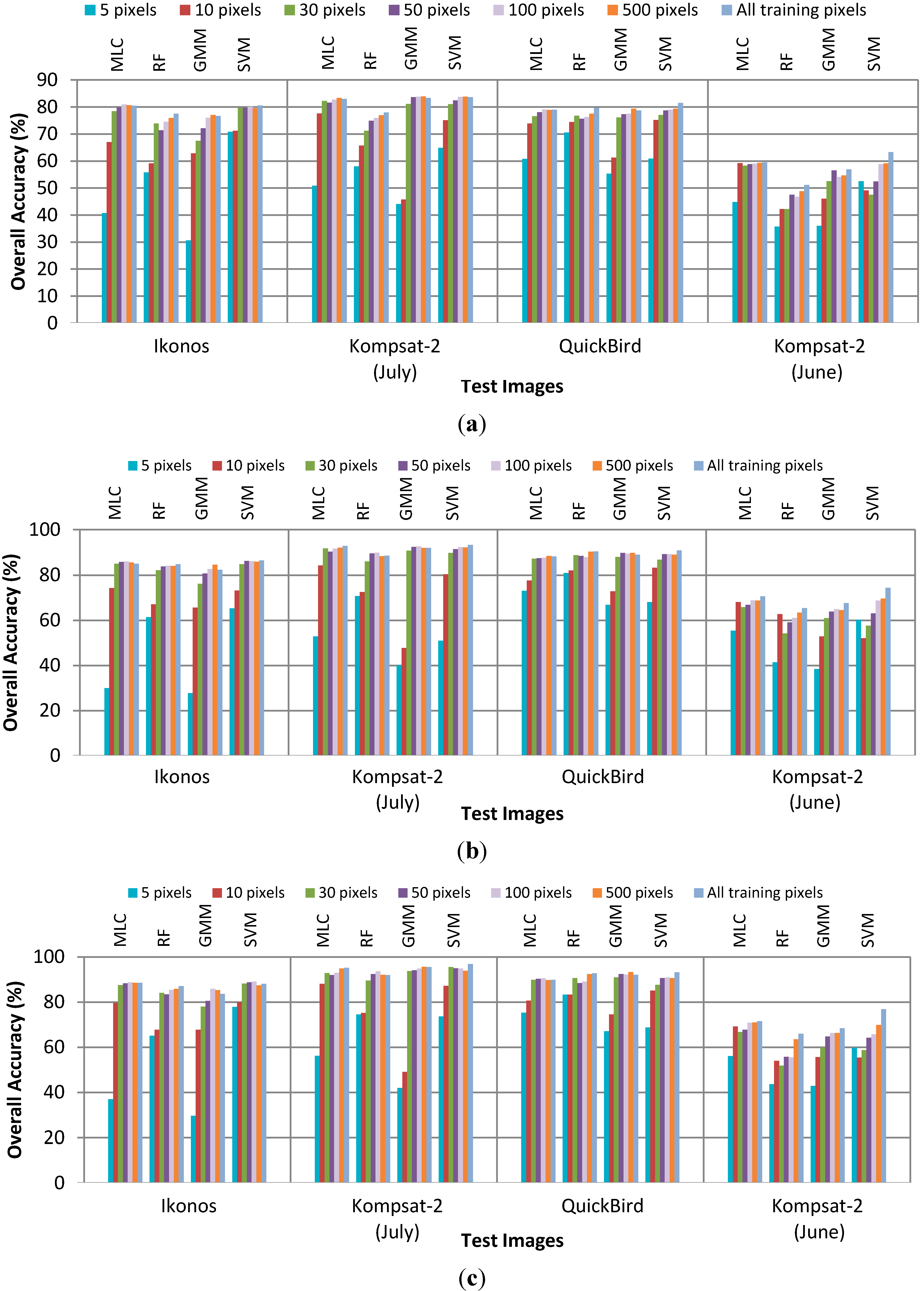
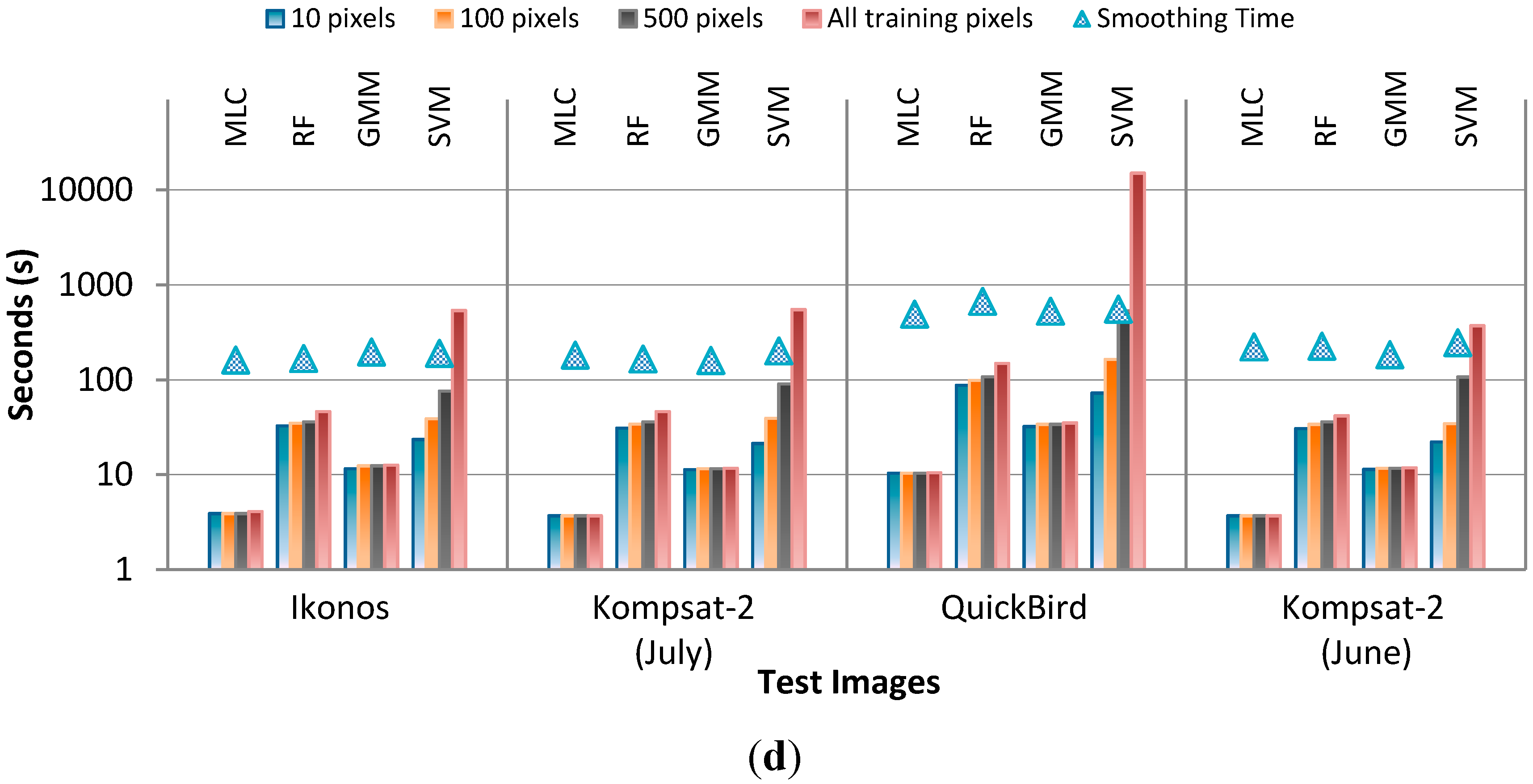
4.1. Performance without Smoothing

Overall per-pixel accuracies for all base classifiers are given in Figure 2. SVM provides the highest performance for all images (Ikonos 80.6%, Kompsat-2 July 83.6%, QuickBird 81.5%, Kompsat-2 June 63.3%). Classification performance for Kompsat-2 June is noticeably lower (with all methods). This is mainly because of the imperfect acquisition period. In June, most of the crop types are in the early planting season, and bare soil dominates the visible surface, and hence the spectral response. SVM consistently works best, which suggests a systematic, albeit small, advantage. Note however that this comes at the price of significantly longer processing time (Figure 3, cf. Section 4.5).
Figure 2. Performances without smoothing, (a) Overall accuracies, and (b) kappa indices.
Remotesensing 07 05611 g002
Figure 3. Processing time of each method.
Remotesensing 07 05611 g003
For completeness we point out a few more details: the performance of GMM depends on the unsupervised initial clustering used to initialize the GMM procedure; the results of RF vary slightly over different runs as a consequence of the randomness in the classifier (for the Kompsat-2 June image we observe a somewhat larger spread with standard deviation 1.6%). The reported results of RF in Figure 2 are means over 20 runs. Also, we stress that RF classifiers are not as “standardized” as others and results may vary depending on the implementation.
MLC provided good results in our tests as a base classifier. This indicates that for our crop classes the assumption of a unimodal Gaussian distribution holds well; however, this rather restrictive assumption might not apply for other crop types. Note also that the MLC and GMM methods suffer from the curse of dimensionality, i.e., for larger feature sets that also include texture filters etc., it might not be possible to learn them reliably from a reasonable number of training samples.

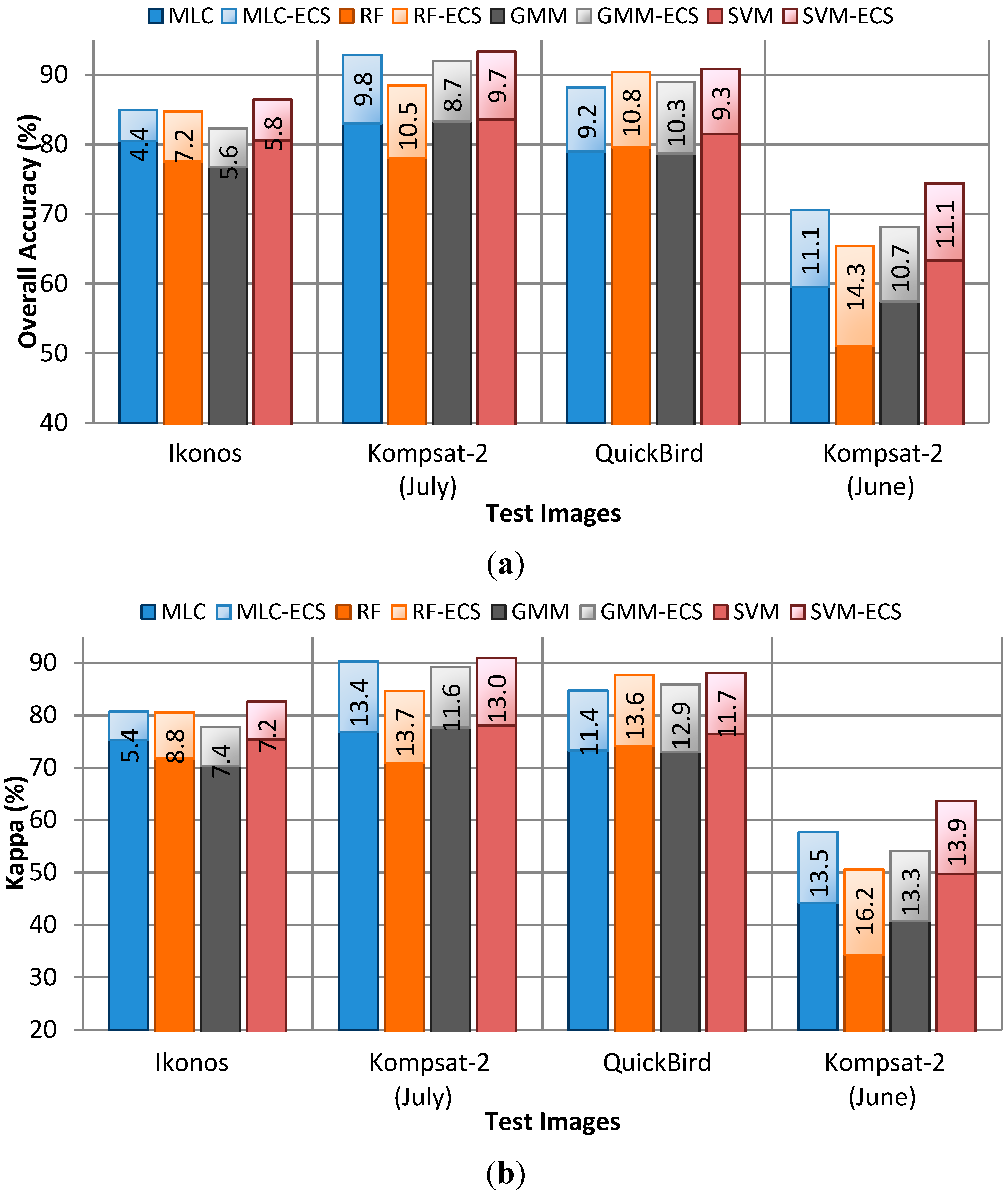
4.2. Performance of CRF Smoothing

We observe significant performance improvements with CRF smoothing, both for linear contrast sensitive (LCS) or exponential contrast smoothing (ECS), see Figure 4 and Figure 5. According to the signed rank test over all 16 trials (4 methods × 4 datasets) the differences are highly significant (p-value 0.0004). The best results overall are achieved with the combination SVM-ECS (Ikonos 86.4%, Kompsat-2 July 92.4%, QuickBird 90.8%, Kompsat-2 June 74.4%).
Figure 4. Performance improvements after CRF contrast smoothing. (a) Overall accuracies, and (b) kappa indices.
Remotesensing 07 05611 g004
Figure 5. Performance improvements after CRF exponential smoothing. (a) Overall accuracies, and (b) kappa indices.
Remotesensing 07 05611 g005
In our tests the improvement in overall classification accuracy due to smoothing lies between 5% and 14%, with a mean of almost 10%. When comparing different smoothing functions, ECS dominates LCS in all runs except for two cases on the Ikonos dataset (Figure 5). Even though there is a systematic difference between LCS and ECS according to the signed rank test (p-value 0.002), the performance difference between the two is small (<2%), and perhaps not very relevant for our problem. Still, ECS also requires fewer user parameters (cf. Section 4.5). Overall, we may conclude, in line with other studies, that also for our task of crop classification it is vital to use smoothing, whereas the exact choice of the potential is less critical.

4.3. CRF vs. Parcel-Based Smoothing

The results in Figure 6 indicate that state-of-the-art parcel-based smoothing consistently gives the best results for all four data sets. This is not surprising given that strategy utilizes land parcel information in addition to image data, which induces ground-truth segmentation boundaries and greatly increases the redundancy per parcel. Again, the gains are consistent across different base classifiers and datasets and highly significant (p-value 0.0004). On average, SVM-ECS results are 2.5% lower in OA and 3.5% lower in Kappa.
Figure 6. Performance comparison of three strategies, without-smoothing, CRF smoothing, and parcel-based smoothing.
Remotesensing 07 05611 g006
Although there clearly is a difference, it is relatively small compared to the amount of additional information used by the parcel-based method. Purely data-driven classification may therefore be a useful alternative for many practical applications: gathering parcel boundaries and keeping them up-to-date is rather time consuming, especially in operational applications, which typically cover much larger areas. It also requires experienced operator(s), and the digitized boundaries may (partially) require validation in the field. Furthermore, in valuable agricultural regions where multiple crops are cultivated in one season, parcel information must be updated several times per year. Considering these requirements, we believe that state-of-the-art methods without parcel boundaries, such as the proposed smoothing with graph cuts, are an excellent option for many tasks. In our experiments they achieve results almost on par with those of parcel-based classification, and absolute accuracies that should allow for their use in many practical applications (>85% accuracy for images acquired at the correct time of year).

4.4. Discussion of the Classification Results

In this section, we go through the confusion matrices, user’s accuracies (UA) and producer’s accuracies (PA) in more detail. Among the data-driven methods, we only discuss the most promising ones (cf. Section 4.2). Generally, among our crop types, confusions happen mostly between sugar beet, tomato, pasture, and corn. This can be explained by the similar spectral response characteristics of these crop types and the confusion of crop reflectance with bare soil during the early planting season of the crops (e.g., Kompsat-2 June image). Detailed comments for each image are provided in the following.
Figure 7 shows the outputs for the Ikonos image, and Table 1 shows the corresponding confusion matrix of SVM-ECS. The total number of reference pixels used for the classification is 1,840,093. The major source of error is confusion between pasture and corn. Of the total 257,703 pasture pixels, only 153,932 are correctly classified. A similar behavior is observed for sugar beet, in this case due to confusions with tomato, which is spectrally similar. Overall, the classifier seems to be biased towards large classes, leading to high PA (up to 97% and always above a remarkable 82%), but for some classes low UA (many false negatives). It may be possible to mitigate this behavior by additional prior knowledge about the expected (relative) frequency of different crop types.
Figure 7. (a) Ikonos test image (RGB, 2771 × 2324 pixels, acquired on 15 July 2004), and the (b) reference map. Thematic output maps of, (c) SVM without smoothing, (d) SVM-LCS, (e) SVM-ECS, and (f) parcel-based strategy with SVM without smoothing.
Remotesensing 07 05611 g007
Table 1. Confusion matrix of SVM-ECS classification for Ikonos test image.
CornPastureRiceSugar BeetWheatTomatoRow TotalUA
Corn467,947350043145373372232481,90097.1%
Pasture85,881153,93234287624711,322257,70359.7%
Rice17122143,324402021181145,75998.3%
Sugar Beet1120389861,94919235,838101,98960.7%
Wheat7250652469429383,8223838397,87396.5%
Tomato88552681082118165,228378,255454,86983.2%
Col. Total570,216157,787151,23864,339464,847431,6661,840,093
PA82.1%97.6%94.8%96.3%82.6%87.6%
Overall Accuracy: 86.37% Kappa Index: 82.65%
The classification outputs for the Kompsat-2 July image and the confusion matrix of SVM-ECS are shown in Figure 8 and Table 2, respectively. The total number of reference pixels is 901,107. The results are similar. Once again, a major confusion is observed between tomato and sugar beet due to their similar spectral responses. Also important is the confusion of corn with rice and wheat. PA is generally high (>84%), but rare classes tend to be swallowed and have low UA.
Figure 8. (a) Kompsat-2 July test image (RGB, 2,721 × 2,258 pixels, acquired on 11 July 2008), and the (b) reference map. Thematic output maps of, (c) SVM without smoothing, (d) SVM-LCS, (e) SVM-ECS, and (f) parcel-based strategy with SVM without smoothing.
Remotesensing 07 05611 g008
Table 2. Confusion matrix of SVM-ECS classification for Kompsat-2 July test image.
CornPastureRiceSugar BeetWheatTomatoRow TotalUA
Corn18,5011059988597468918934,06954.3%
Pasture346204.292261851858799214,43695.3%
Rice024212,35215922840214,25299,1%
Sugar Beet266143177,8111829578,39999.3%
Wheat227.06845717318,3370325,90197.7%
Tomato16851.446491511,5584806964034,05028.3%
Col. Total20,820212.949228,00492,426336,88510,023901,107
PA88.9%95.9%93.1%84.2%94.5%96.2%
Overall Accuracy: 93.32% Kappa Index: 90.95%
The confusion matrix for the QuickBird test image is given in Table 3. The classification results are illustrated in Figure 9. The total number of reference pixels included is 4,811,904. Main sources of error are confusions between rice and wheat, and between sugar beet and tomato. In this case, the bias toward abundant classes is less severe (worst UA > 72%). PA nevertheless stays high (rice 74%, others > 88%). We note that for the corn class we get 95.7% PA and 95.5% UA, which is quite remarkable for a method using only four broad multispectral channels.
Figure 9. (a) QuickBird test image (RGB, 4,666 × 3,873 pixels, acquired on 13 August 2004), and the (b) reference map. Thematic output maps of, (c) SVM without smoothing, (d) SVM-LCS, (e) SVM-ECS, and (f) parcel-based strategy with SVM without smoothing.
Remotesensing 07 05611 g009
Table 3. Confusion matrix of SVM-ECS classification for QuickBird test image.
CornPastureRiceSugar BeetWheatTomatoRow TotalUA
Corn1,034,38627,3633313829983573041,083,03095.5%
Pasture31,127408,470347683295456,790500,37181.6%
Rice840311,5174317,4934078333,21593.5%
Sugar Beet222938,534167,84225924,118230,98472.7%
Wheat9927100029,39111111,205,72274,1431,321,29491.3%
Tomato5029135237,945832449,8141,240,5461,343,01092.4%
Col. Total1,080,775438,194421,047178,8321,286,0771,406,9794,811,904
P.A.95.7%93.2%74.0%93.9%93.8%88.2%
Overall Accuracy: 90.78% Kappa Index: 88.14%
Compared with the other three test images, the degree of confusion is higher for the Kompat-2 June image (Figure 10 and Table 4). As mentioned before, this is mainly due to the acquisition date shortly after the early planting period, causing distorted spectral responses of the different crop types. As plants are at an early growth stage, they are harder to discriminate and they only partially cover the ground, such that bare soil is visible and disturbs the classification. Another more technical factor is the limited number of reference data for two classes, corn and tomato. Possibly the training set might be insufficient to learn these two classes. The total number of reference pixels for validation is 1,186,694. For the small classes (corn and tomato) classification essentially fails. Furthermore, there are important confusions between pasture and wheat. Still, even in this challenging setting the larger classes reach UA and PA of 85% or more, and a respectable 74% of all pixels are classified correctly. One can speculate that with an image taken only two weeks later, satisfactory results might be possible.
Figure 10. (a) Kompsat-2 June test image (RGB, 2721 × 2258 pixels, acquired on 13 June 2008), and the (b) reference map. Thematic output maps of, (c) SVM without smoothing, (d) SVM-LCS, (e) SVM-ECS, and (f) parcel-based strategy with SVM without smoothing.
Remotesensing 07 05611 g010
Table 4. Confusion matrix of SVM-ECS classification for Kompsat-2 June test image.
CornPastureRiceSugar BeetWheatTomatoRow TotalUA
Corn372716594527205889013,44627.7%
Pasture6652153,4411215400152,83126433,21,08847.8%
Rice2069106230,478362332,1691006269,45185.5%
Sugar Beet6235213926399,92860383501118,10484.6%
Wheat131260,03526733603393,3851254462,26285.1%
Tomato00076142253234396.2%
Col. Total19,995215,886234,480115,350590,32610,6571,186,694
PA18.6%71.1%98.3%86.6%66.6%21.1%
Overall Accuracy: 74.43% Kappa Index: 63.58%
Comparing the performances for Ikonos, QuickBird and Kompsat-2 July images, we achieved the best classification performance for the Kompsat-2 July dataset (OA: 93.32% and Kappa: 90.95%). Indeed, this is a result we expected, because the number of reference pixels for classes corn and tomato is lower in 2008 compared to 2004; therefore, confusions between these two classes have a smaller influence on the overall performance.

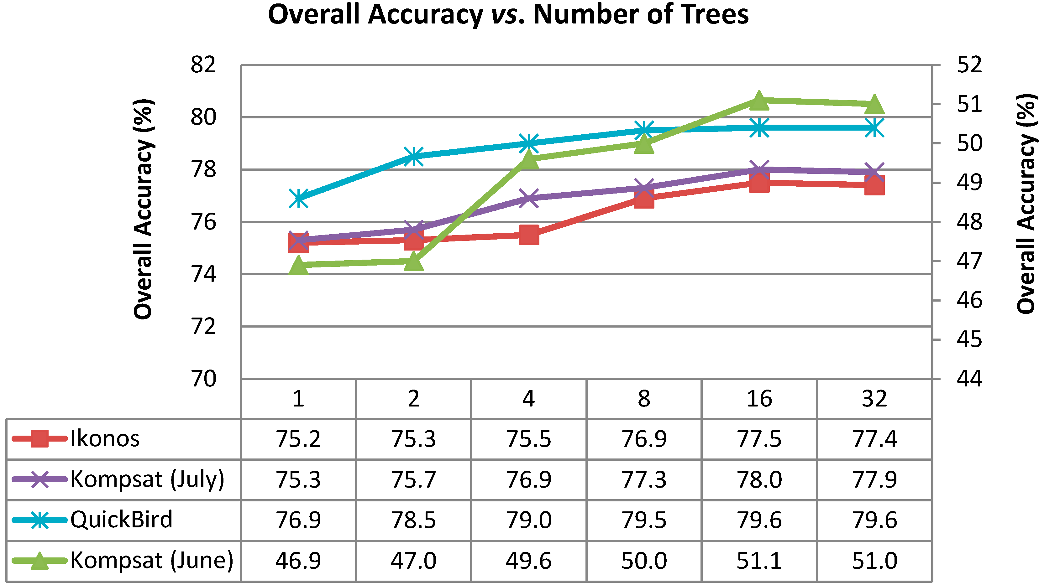
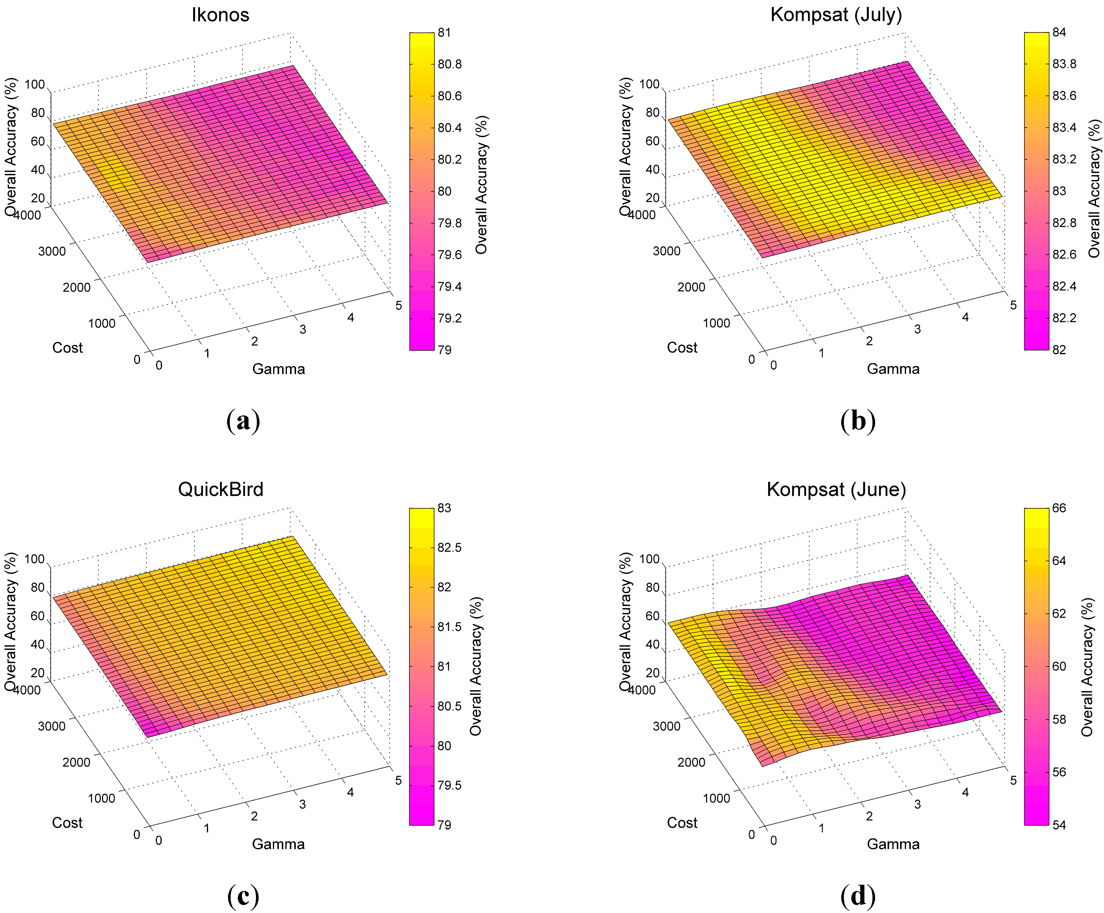
4.5. Sensitivity to Parameters

Like any classification pipeline ours requires a small number of parameters to be set by the user. To assess the robustness with respect to this user input we ran a parameter study. We limit ourselves to the main parameters, whereas values that would normally not be changed for different problems and datasets remain fixed, see Table 5 and Table 6.
Table 5. Parameter test settings of each classifier without smoothing.
ClassifierParametersOptionsTest
GMMNum. of components≥22…8
Covariance type“Full” “Diagonal”“Full” (Default)
Shared covariance“Yes”
“No”
“No” (Default)
Regularization term≥010−5
Termination tolerance≥010−6 (Default)
RFNum. of trees≥11…50
Num. of variables (n) to select for each decision split n (Default)2
Minimum num. of observations per tree leaf≥11 (Default)
SVMKernel type“Linear”
“Polynomial”
“Radial Function”
“Sigmoid”
“Radial Function”
Gamma≥00…5
Cost≥00…4000
Termination tolerance≥010−3 (Default)
Table 6. Parameter settings of each classification with smoothing.
Smoothing ParametersOptionsSet
Linear Contrast SensitiveGaussian standard deviation (σ)>00,5 (Default)
truncated linear potential function constant (ϕ)2 ≥ ϕ ≥ 00…2
Smoothing constant (γ)>01..4
Neighborhood Connectivity4 or 88 (Default)
Exponential Contrast SensitiveSmoothing constant (γ)>01…12
Neighborhood Connectivity4 or 88 (Default)
For the GMM classifier, the main parameter is the number of Gaussians. Although a number of approaches exist for estimating the number of components, e.g., [66], our tests performed with different numbers of components reveal that this parameter can be set across a range of values (3–5) without large impact on the performance (Figure 11). We think that the reason is the binary tree quantization clustering [55] used to initialize the GMM parameters. For the remaining parameters, we use default values: independent full covariance matrices for each component, and a small regularization term (10−5) to ensure positive-definite covariance matrices.
Figure 11. Overall accuracy vs. number of components of GMM. (The results of Kompsat-2 June image are presented on the right-y axis to improve visibility).
Remotesensing 07 05611 g011
For the RF classifier, the number of trees is a user-defined parameter. Figure 12 shows that, except for an overly small number of trees (≤4), the performance is rather stable. Other parameters of the RF classifier are set to fixed defaults, since preliminary tests showed that they do not significantly affect the performance (<0.5%).
Figure 12. Overall accuracy vs. number of trees of RF classifier. (The results of Kompsat-2 June image are presented on the right y axis to improve visibility).
Remotesensing 07 05611 g012
For the SVM, we prefer the radial basis function (RBF) kernel, which has only one additional parameter compared to the linear kernel, and is known to perform well across a variety of classification tasks (e.g., [47,67,68]). For the two parameters—the kernel width gamma and the cost for misclassified samples—we run a grid search (Figure 13). The results in Figure 13 confirm that different combinations of SVM parameters affect the overall accuracies at most 3% for Ikonos, Kompsat July and QuickBird test images, and the performance is rather consistent (within 2.5%) across a range of values. The largest differences in classification accuracy, up to 11%, are observed for the Kompsat June image. It is interesting to note that the trend is similar to the ones observed for Ikonos and Kompsat July, namely that the main failure mode is a too large kernel width. We conclude that it is easy to choose a parameter set that generalizes across different images, and set, Gamma = 0.5, Cost = 2100 for all our tests.
Figure 13. Sensitivity of SVM parameters with respect to overall accuracy. Please note the different scales of the color bars.
Remotesensing 07 05611 g013
Table 6 summarizes the parameters used for the CRF smoothing approaches. We fix the connectivity to the 8-neighborhood for both of the smoothing strategies; it has been repeatedly observed that it performs very similarly to the 4-neighborhood, but slightly reduces metrication artifacts along class boundaries.
We also fix the standard deviation of the gradient filter to the standard value of 0.5. The parameters that we vary are the truncation of the linear potential function (ϕ) and the smoothness weight (γ). Our tests reveal that the best results are achieved when ϕ is set to 0, i.e., no penalty at intensity gradients above 50% of the observed maximum. Figure 14 shows how the overall accuracies of SVM-LCS change with respect to different truncation values. We observe that overall accuracies are all negatively affected by large ϕ values, especially with stronger smoothing.
We find that the performance across a range of smoothness weights γ is similar, both for LCS and ECS. However, we also observe that the performances drop slightly when over-smoothing occurs and this fact is mainly due to the relatively small-sized parcels.
Figure 14. Overall accuracies of SVM-LCS vs. truncated linear potential function constant (ϕ). Only four smoothing constants (γ = 1, 2, 3, and 4) are illustrated to increase readability.
Remotesensing 07 05611 g014
In our last experiment, we test the effect of training set size on classification accuracy. We randomly selected, at each run and for each class, a number of training samples (5, 10, 30, 50, 100, and 500 pixels) from the whole training set, and ran the classification without smoothing, with CRF smoothing, and with parcel-based smoothing. Figure 15 shows the classification performance as a function of training set size. While too-small training sets are obviously detrimental, all classifiers perform acceptably with 50 training samples per class, and with 100 training samples almost reach the performance achievable with the full training sets, which have >10,000 pixels.
An exception is the Kompsat-2 June image, where the classification performance does not seem to saturate, indicating that the class boundaries are indeed more complicated due to the early acquisition date. Also note that the results with smoothing follow the ones without smoothing—even when the performance of the unaries saturates, smoothing still helps, but weaker unaries learned from overly small training sets also benefit from smoothing.
Figure 15d shows how training set size affects the computation times during testing. As expected, runtimes of MLC and GMM are independent of the training set size, as the model complexity does not change with more samples; RF takes slightly longer with more training data, as the trees can grow deeper; and SVM is strongly affected, since the number of support vectors grows with the training set size. In the worst case (QuickBird) the processing time reaches ≈ 4 h. Note, all timings are indicative and depend on the specific implementation. In particular, multiclass SVMs as well as RF naturally lend themselves to parallelization. The time spent for smoothing is practically constant in each image and slightly longer for the QuickBird data, since with a fixed neighborhood definition it depends only on the number of pixels and the number of classes.
Figure 15. Performance vs. training size. (a) Without any smoothing, (b) with ECS smoothing, and (c) parcel-based strategy. (d) Speed of processing vs. training size. “All training pixels” refer to: 48,825; 43,543; 135,752, and 14,251 pixels for the Ikonos, Kompsat-2 July, QuickBird and Kompsat-2 June images, respectively.
Remotesensing 07 05611 g015aRemotesensing 07 05611 g015b

5. Conclusions

We have investigated the possibility of classifying agricultural crops at high spatial resolution, using only a single multispectral image as input. In an extensive evaluation, we find that (i) smoothing based on known parcel boundaries, as expected, delivers the best result, (ii) purely data-driven smoothing comes close to the parcel-based approach and could in many applications be a valuable alternative, (iii) if the images are taken at the right time of year, i.e., after the crops have developed sufficient size and coverage, standard classifiers achieve satisfactory classification accuracy, using only the R, G, B and NIR bands.
The four different tested classifiers deliver rather similar results. SVM provides the best performance in all cases, but at the cost of longer processing times. Our tests also show that CRF smoothing increases the overall classification performance by about 10%. The results indicate that ECS smoothing slightly (≈2%) outperforms LCS smoothing. Notably, the difference between parcel-based smoothing and CRF smoothing is rather small (≈2.5%). Considering the effort to obtain up-to-date parcel boundary information, CRF smoothing seems to be an interesting alternative unless reliable parcel boundaries are already available.
A further finding is that moderate training sets sizes of about 100 pixels per class are sufficient, in spite of the rather coarse spectral resolution. Note however that it might in practice be easier to collect larger training sets, in order to make sure that the samples are representative of the full class distribution.
This study also highlights the importance of image acquisition dates based on crop phenology. For most crop types, it is better to be in their highest ripening period during image acquisition. Such a setup reduces the visibility of bare soil and guarantees a high coverage of the parcels with crops. In this study, we observe that in Mediterranean climate images taken in June provide poor classification results compared to those acquired in July and August. The spectral confusions between (early) crops and bare soil are most apparent in June, and are a major source of classification errors. However, we should also stress that there may be large variations of crop phenology among different crop types for different geographic locations and times. There might be crop combinations for which no single best acquisition period exists; or the ideal time window might be very short or fall into an unfavorable weather period, such that it becomes a matter of luck to obtain cloud-free VHR images. In such circumstances one might have to revert to multitemporal datasets [8,52] and/or other sensor types such as SAR.
Considering the individual crop types used in our study, confusions are principally observed between pasture/corn, rice/sugar beet, tomato/sugar beet, and corn/sugar beet. We explain this fact mainly by similar spectral characteristics of these classes under the limited spectral resolution (B, G, R, NIR) of the images. This, of course, can be mitigated to some extent by collecting more training samples or by integrating additional features and color spaces [69] into the classification framework. Currently, we have not tested the impact of additional information, but we plan to do so in the future.
On a more technical note, we believe that high-throughput classification is possible with the tested methods, but this would require parallel implementations, probably using GPUs. The obvious starting point for an efficient implementation is the pixel-wise computation of the unaries, but other multilabel energy minimization methods like FastPD [70] could potentially also bring down computation times.

Acknowledgments

The Ikonos and QuickBird images are funded by OYP research project BAP-08-11-DPT2002K120510, and we thank Prof. Dr. Mustafa Turker for his contribution during the collection of reference data of the Ikonos and QuickBird images. The Kompsat-2 images are funded by scientific project DAP-2008-07-02-07 and we thank the farmers and staff working in the irrigation department of the region for contributing to our study with respect to the field observations of Kompsat-2 images.

Author Contributions

Asli Ozdarici-Ok and Ali Ozgun Ok developed the original idea for the study and collected the data. All three authors contributed to the implementation. Ali Ozgun Ok and Asli Ozdarici-Ok carried out the experiments. All three authors planned the paper. Asli Ozdarici-Ok drafted the initial manuscript, which was then revised by all authors. All authors read and approved the final manuscript.

Conflicts of Interest

The authors declare no conflict of interest.

References

  1. Lobell, D.B.; Asner, G.P. Climate and management contributions to recent trends in U.S. agricultural yields. Science 2003, 299. [Google Scholar] [CrossRef]
  2. Penã-Barragán, J.M.; Ngugi, M.K.; Plant, R.E.; Six, J. Object-based crop identification using multiple vegetation indices, textural features and crop phenology. Remote Sens. Environ. 2011, 115, 1301–1316. [Google Scholar] [CrossRef]
  3. Wilkinson, G.G. Results and implications of a study of fifteen years of satellite image classification experiments. IEEE Trans. Geosci. Remote Sens. 2005, 43, 433–440. [Google Scholar] [CrossRef]
  4. Lu, D.; Weng, Q. A survey of image classification methods and techniques for improving classification performance. Int. J. Remote Sens. 2007, 28, 823–870. [Google Scholar] [CrossRef]
  5. Lillesand, M.; Kiefer, R.W.; Chipman, J.W. Remote Sensing and Image Interpretation, 6th ed.; Wiley: Hoboken, NJ, USA, 2004; p. 638. [Google Scholar]
  6. Muñoz-Marí, J.; Bovolo, F.; Gómez-Chova, L.; Bruzzone, L.; Camp-Valls, G. Semisupervised one-class support vector machines for classification of remote sensing data. IEEE Trans. Geosci. Remote Sens. 2010, 48, 3188–3197. [Google Scholar] [CrossRef]
  7. Turker, M.; Ozdarici, A. Field-based crop classification using SPOT4, SPOT5, IKONOS, and QuickBird imagery for agricultural areas: A comparison study. Int. J. Remote Sens. 2011, 32, 9735–9768. [Google Scholar] [CrossRef]
  8. Ozdarici Ok, A.; Akyurek, Z. A segment-based approach to classify agricultural lands by using multitemporal optical and microwave data. Int. J. Remote Sens. 2012, 33, 7184–7204. [Google Scholar]
  9. Song, M.; Civco, D.L.; Hurd, J.D. A competitive pixel-object approach for land cover classification. Int. J. Remote Sens. 2005, 26, 4981–4997. [Google Scholar] [CrossRef]
  10. Janssen, L.L.F.; Jaarsma, M.N.; Van Der Linden, E.T.M. Integrating topographic data with remote sensing for land-cover classification. Photogram. Eng. Remote Sens. 1990, 56, 1503–1506. [Google Scholar]
  11. Aplin, P.; Atkinson, P.M. Sub-pixel land cover mapping for per-field classification. Int. J. Remote Sens. 2001, 22, 2853–2858. [Google Scholar] [CrossRef]
  12. Smith, G.M.; Fuller, R.M. An integrated approach to land cover classification: An example in the Island of Jersey. Int.l J. Remote Sens. 2001, 22, 3123–3142. [Google Scholar] [CrossRef]
  13. Lloyd, C.D.; Berberoglu, S.; Curran, P.J.; Atkinson, P.M. A comparison of texture measures for the per-field classification of Mediterranean land cover. Int. J. Remote Sens. 2004, 25, 3943–3965. [Google Scholar] [CrossRef]
  14. Cheng, H.D.; Jiang, X.H.; Sun, Y.; Wang, J. Color image segmentation: Advances and prospects. Pattern Recognit. 2001, 12, 2259–2281. [Google Scholar] [CrossRef]
  15. Gong, P.; Marceau, D.; Howarth, P.J. A comparison of spatial feature extraction algorithms for land-use mapping with SPOT HRV data. Remote Sens. Environ. 1992, 40, 137–151. [Google Scholar] [CrossRef]
  16. Gong, P.; Howarth, P.J. Frequency-based contextual classification and grey-level vector reduction for land-use identification. Photogram. Eng. Remote Sens. 1992, 58, 423–437. [Google Scholar]
  17. Yu, Q.; Gong, P.; Clinton, N.; Biging, G.; Schirokauer, D. Object-based detailed vegetation mapping using high spatial resolution imagery. Photogram. Eng. Remote Sens. 2006, 72, 799–811. [Google Scholar] [CrossRef]
  18. Rydberg, A.; Borgefors, G. Integrated method for boundary delineation of agricultural fields in multispectral satellite images. IEEE Trans. Geosci. Remote Sens. 2001, 39, 2514–2520. [Google Scholar] [CrossRef]
  19. Wang, L.; Sousa, W.P.; Gong, P.; Biging, G.S. Comparison of IKONOS and QuickBird images for mapping mangrove species on the Caribbean coast of Panama. Remote Sens. Environ. 2004, 91, 432–440. [Google Scholar] [CrossRef]
  20. Lee, J.Y.; Warner, T.A. Segment based image classification. Int. J. Remote Sens. 2006, 27, 3403–3412. [Google Scholar] [CrossRef]
  21. Castillejo-González, I.L.; López-Granados, F.; García-Ferrer, A.; Peña-Barragán, J.M.; Jurado-Expósito, M.; de la Orden, M.S.; González-Audicana, M. Object- and pixel-based analysis for mapping crops and their agro-environmental associated measures using QuickBird imagery. Comput. Electron. Agric. 2009, 68, 207–215. [Google Scholar] [CrossRef]
  22. Xiao, P.; Feng, X.; An, R.; Zhao, S. Segmentation of multispectral high-resolution satellite imagery using log gabor filters. Int. J. Remote Sens. 2010, 31, 1427–1439. [Google Scholar] [CrossRef]
  23. Blaschke, T. Object based image analysis for remote sensing. ISPRS J. Photogram. Remote Sens. 2010, 65, 2–16. [Google Scholar] [CrossRef]
  24. Dronova, I.; Gong, P.; Wang, L. Object-based analysis and change detection of major wetland cover types and their classification uncertainty during the low water period at Poyang Lake, China. Remote Sens. Environ. 2011, 115, 3220–3236. [Google Scholar] [CrossRef]
  25. Gao, Y.; Mas, J.F.; Kerle, N.; Pacheco, J.A.N. Optimal region growing segmentation and its effect on classification accuracy. Int. J. Remote Sens. 2011, 32, 3737–3763. [Google Scholar] [CrossRef]
  26. Vieira, M.A.; Formaggio, A.R.; Rennó, C.D.; Atzberger, C.; Aguiar, D.A.; Mello, M.P. Object based image analysis and data mining applied to a remotely sensed Landsat time-series to map sugarcane over large areas. Remote Sens. Environ. 2012, 123, 553–562. [Google Scholar] [CrossRef]
  27. De Castro, A.I.; López-Granados, F.; Jurado-Expósito, M. Broad-scale cruciferous weed patch classification in winter wheat using QuickBird imagery for in-season site-specific control. Precis. Agric. 2013, 14, 392–413. [Google Scholar] [CrossRef]
  28. Zhong, L.; Gong, P.; Biging, G.S. Efficient corn and soybean mapping with temporal extendability: A multi-year experiment using Landsat imagery. Remote Sens. Environ. 2014, 140, 1–13. [Google Scholar] [CrossRef]
  29. Peña, J.M.; Gutiérrez, P.A.; Hervás-Martínez, C.; Six, J.; Plant, R.E.; López-Granados, F. Object-based image classification of summer crops with machine learning methods. Remote Sens. 2014, 6, 5019–5041. [Google Scholar] [CrossRef]
  30. Clinton, N.; Holt, A.; Scarborough, J.; Yan, L.I.; Gong, P. Accuracy assessment measures for object-based image segmentation goodness. Photogram. Eng. Remote Sens. 2010, 76, 289–299. [Google Scholar] [CrossRef]
  31. Schindler, K. An overview and comparison of smooth labeling methods for land-cover classification. IEEE Trans. Geosci. Remote Sens. 2012, 50, 4534–4545. [Google Scholar] [CrossRef]
  32. Boykov, Y.; Veksler, O.; Zabih, R. Fast approximate energy minimization via graph cuts. IEEE Trans. Pattern Anal. Mach. Intell. 2001, 23, 1222–1239. [Google Scholar] [CrossRef]
  33. Tyagi, M.; Bovolo, F. A context-sensitive clustering technique based on graph-cut initialization and expectation-maximization algorithm. IEEE Geosci. Remote Sens. Lett. 2008, 5, 21–25. [Google Scholar] [CrossRef]
  34. Bai, J.; Xiang, S.; Pan, C. A graph-based classification method for hyperspectral images. IEEE Trans. Geosci. Remote Sens. 2013, 51, 803–817. [Google Scholar] [CrossRef]
  35. Zhong, P.; Wang, R. Learning conditional random fields for classification of hyperspectral images. IEEE Trans. Image Process. 2010, 19, 1890–1907. [Google Scholar] [CrossRef] [PubMed]
  36. Zhong, Y.; Zhao, J.; Zhang, L. A hybrid object-oriented conditional random field classification framework for high spatial resolution remote sensing imagery. IEEE Trans. Geosci. Remote Sens. 2014, 52, 7023–7037. [Google Scholar] [CrossRef]
  37. Zhao, J.; Zhong, Y.; Zhang, L. Detail-preserving smoothing classifier based on conditional random fields for high spatial resolution remote sensing imagery. IEEE Trans. Geosci. Remote Sens. 2015, 53, 2440–2452. [Google Scholar] [CrossRef]
  38. Moser, G.; Serpico, S.B. Combining support vector machines and markov random fields in an integrated framework for contextual image classification. IEEE Trans. Geosci. Remote Sens. 2013, 51, 2734–2752. [Google Scholar] [CrossRef]
  39. Boykov, Y.; Jolly, M.P. Interactive graph cuts for optimal boundary and region segmentation of objects in ND images. In Proceedings of International Conference on Computer Vision, Vancouver, Canada, 7–14 July 2001; pp. 105–112.
  40. Rother, C.; Kolmogorov, V.; Blake, A. Grabcut: Interactive foreground extraction using iterated graph cuts. ACM Trans. Graph. 2004, 23, 309–314. [Google Scholar] [CrossRef]
  41. Szeliski, R.; Zabih, R.; Scharstein, D.; Veksler, O.; Kolmogorov, V.; Agarwala, A.; Tappen, M.; Rother, C. A comparative study of energy minimization methods for markov random fields with smoothness-based priors. IEEE Trans. Pattern Anal. Mach. Intell. 2008, 30, 1068–1080. [Google Scholar] [CrossRef] [PubMed]
  42. Vapnik, V. The Nature of Statistical Learning Theory; Springer-Verlag: New York, NY, USA, 1995. [Google Scholar]
  43. Vapnik, V. Statistical Learning Theory; Springer-John Wiley: New York, NY, USA, 1998. [Google Scholar]
  44. Tso, B.; Mather, P.M. Classification Methods for Remotely Sensed Data, 2nd ed.; Taylor & Francis Group, LLC: Danvers, MA, USA, 2009. [Google Scholar]
  45. Hsu, C.-W.; Lin, C.-J. A comparison of methods for multi-class support vector machines. IEEE Trans. Neural Netw. 2002, 13, 415–425. [Google Scholar] [CrossRef] [PubMed]
  46. Foody, G.M.; Mathur, A. Toward intelligent training of supervised image classifications: Directing training data acquisition for SVM classification. Remote Sens. Environ. 2004, 93, 107–117. [Google Scholar] [CrossRef]
  47. Pal, M.; Mather, P.M. Support vector machines for classification in remote sensing. Int. J. Remote Sens. 2005, 26, 1007–1011. [Google Scholar] [CrossRef]
  48. Pal, M. Support vector machine-based feature selection for land cover classification: A case study with DAIS hyperspectral data. Int. J. Remote Sens. 2006, 27, 2877–2894. [Google Scholar] [CrossRef]
  49. Archer, K.J. Empirical characterization of random forest variable importance measure. Comput. Stat. Data Anal. 2008, 52, 2249–2260. [Google Scholar] [CrossRef]
  50. Breiman, L. Random Forests. Mach. Learn. 2001, 45, 5–32. [Google Scholar] [CrossRef]
  51. Rodriguez-Galiano, V.F.; Ghimire, B.; Rogan, J.; Chica-Olmo, M.; Rigol-Sanchez, J.P. An assessment of the effectiveness of a random forest classifier for land-cover classification. ISPRS J. Photogram. Remote Sens. 2012, 67, 93–104. [Google Scholar] [CrossRef]
  52. Long, J.A.; Lawrence, R.L.; Greenwood, M.C.; Marshall, L.; Miller, P.R. Object-oriented crop classification using multitemporal ETM+ SLC-off imagery and random forest. GIScience Remote Sens. 2013, 50, 418–436. [Google Scholar]
  53. Sonobe, R.; Tani, H.; Wang, X.; Kobayashi, N.; Shimamura, H. Random forest classification of crop type using multi-temporal TerraSAR-X dual-polarimetric data. Remote Sens. Lett. 2014, 5, 157–164. [Google Scholar] [CrossRef]
  54. McLachlan, G.; Peel, D. Finite Mixture Models; John Wiley, Sons Inc.: Hoboken, NJ, USA, 2000. [Google Scholar]
  55. Orchard, M.T.; Bouman, C.A. Color quantization of images. IEEE Trans. Signal Process. 1991, 39, 2677–2690. [Google Scholar] [CrossRef]
  56. Brisco, B.; Brown, R.J.; Manore, M.J. Early season crop discrimination with combined SAR and TM data. Can. J. Remote Sens. 1989, 15, 44–54. [Google Scholar]
  57. Aplin, P.; Atkinson, P.M.; Curran, P.J. Fine spatial resolution simulated satellite sensor imagery for land cover mapping in the United Kingdom. Remote Sens. Environ. 1999, 68, 206–216. [Google Scholar] [CrossRef]
  58. Turker, M.; Arikan, M. Sequential masking classification of multi-temporal Landsat7 ETM+ images for field-based crop mapping in Karacabey, Turkey. Int. J. Remote Sens. 2005, 26, 3813–3830. [Google Scholar] [CrossRef]
  59. Hutchinson, C.F. Techniques for combining Landsat and ancillary data for digital classification improvement. Photogram. Eng. Remote Sens. 1982, 48, 123–130. [Google Scholar]
  60. Aplin, P.; Atkinson, P.M.; Curran, P.J. Per-field classification of land use using the forthcoming very fine spatial resolution satellite sensors: Problems and potential solutions. In Advances in Remote Sensing and GIS Analysis; Atkinson, P.M., Tate, N.J., Eds.; John Wiley, Sons: Chichester, UK, 1999; pp. 219–239. [Google Scholar]
  61. Berberoglu, S.; Lloyd, C.D.; Atkinson, P.M.; Curran, P.J. The integration of spectral and textural information using neural networks for land cover mapping in the Mediterranean. Comput. Geosci. 2000, 26, 385–396. [Google Scholar] [CrossRef]
  62. Conrad, C.; Fritsch, S.; Idler, J.; Rücker, G.; Dech, S. Per-field irrigated crop classification in arid central Asia using SPOT and ASTER data. Remote Sens. 2010, 2, 1035–1056. [Google Scholar] [CrossRef]
  63. PCI Geomatica. Geomatica OrthoEngine Course Guide; PCI Geomatics Enterprises Inc.: Richmond Hill, ON, USA, 2009. [Google Scholar]
  64. Pontius, R.G.; Millones, M. Death to Kappa: Birth of quantity disagreement and allocation disagreement for accuracy assessment. Int. J. Remote Sens. 2011, 32, 4407–4429. [Google Scholar] [CrossRef]
  65. Chang, C.-C.; Lin, C.-J. LIBSVM: A library for support vector machines. ACM Trans. Intell. Syst. Technol. 2011, 2, 1–27. Available online: http://www.csie.ntu.edu.tw/~cjlin/libsvm (accessed on 1 May 2015). [Google Scholar]
  66. Figueiredo, M.A.T.; Jain, A.K. Unsupervised learning of finite mixture models. IEEE Trans. Pattern Anal. Mach. Intell. 2002, 24, 381–396. [Google Scholar] [CrossRef]
  67. Yang, X. Parameterizing support vector machines for land cover classification. Photogram. Eng. Remote Sens. 2011, 77, 27–37. [Google Scholar] [CrossRef]
  68. Kavzoglu, T.; Colkesen, I. Destek vektör makineleri ile uydu görüntülerinin siniflandirilmasinda kernel fonksiyonlarinin etkilerinin incelenmesi. Harita Dergisi 2010, 144, 73–82. [Google Scholar]
  69. Tokarczyk, P.; Wegner, J.D.; Walk, S.; Schindler, K. Features, color spaces, and boosting: New insights on semantic classification of remote sensing images. IEEE Trans. Geosci. Remote Sens. 2015, 53, 280–295. [Google Scholar] [CrossRef]
  70. Komodakis, N.; Tziritas, G. Approximate labeling via graph cuts based on linear programming. IEEE Trans. Pattern Anal. Mach. Intell. 2007, 29, 1436–1453. [Google Scholar] [CrossRef] [PubMed]

