Abstract
In this paper, we describe the automatic extraction of centerlines of railroads. Mobile Laser Scanning systems are able to capture the 3D environment of the rail tracks with a high level of detail. Our approach first detects laser points that were reflected by the rail tracks, by making use of local properties such as parallelism and height in relation to neighboring objects. In the modeling stage, we present two approaches to determine the centerline location. The first approach generates center points in a data-driven manner by projecting rail track points to the parallel track, and taking the midpoint as initial center point. Next, a piecewise linear function is fitted through the center points to generate center points at a regular interval. The second approach models the rail track by fitting piecewise 3D track models to the rail track points. The model consists of a pair of two parallel rail tracks. The fitted pieces are smoothened by a Fourier series interpolation function. After that the centerline is implicitly determined by the geometric center of the pair of tracks. Reference data has been used to analyze the quality of our results, confirming that the position of the centerlines can be determined with an accuracy of 2–3 cm.
1. Introduction
The centerline of a rail track is an important element at various stages in the object life of the rail track. In railroad designs, the centerline is used to determine features such as maximum curvature and impact on the environment. Required clearances near the railroad are based on the location of the centerline.
Rail track center lines are also an important data input for track alignment analysis. Rail track operators seek to achieve the most optimal curves to provide a smooth and safe ride for the passengers. Over time, rail tracks tend to shift, thereby degrading the optimal rail path. If the current rail geometry is known, the difference between the optimal path and the actual situation can be computed. Huge machines, such as ballast tempers are used to shift and tilt the rail back into the optimal shape.
The input data for the alignment analysis requires very high accuracy. Traditionally, manual surveys using tachymeters were needed to obtain the data. Currently, mobile mapping systems (MMS) are capable of recording the railroad environment with similar accuracy as manual surveys. Most MMS are equipped with positioning sensors, such as GPS and INS sensors, and image and range sensors, such as cameras and mobile laser scanning (MLS) systems. A broad range of mobile mapping systems is on the market, as described by [1,2]. Although most of the systems are mounted on a car acquiring street level objects, MMS systems can also be mounted on other platforms such as trains and boats [3]. The main difference with manual surveys is that the recorded data is an uninterpreted image or point cloud, instead of a labelled set of interpreted data points.
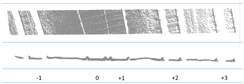
Figure 1.
Varying point density across neighboring rail tracks. Top view (top), cross section (middle), and rail track number (bottom). The mobile mapping system was mounted on a platform driving at track “0”. It is our aim to find the centerlines of all tracks.
The point cloud data can be used for rail track and wires detection, asset management of poles, signs and towers. The promising results on 3D modeling of rail tracks [4] raised the question whether it would be possible to automatically extract the centerline of railroads, with an accuracy better than 1.5 cm standard deviation which is considered to be the accuracy of current semi-automatic or manual measurements. Additional question was if centerline generation is also possible on data where the MMS system is located at a track next to the track of interest. This is of practical importance as it is fairly impossible to drive at every single track of a whole country within a given timeframe without interfering with the regular train schedule. In addition, tracks may be inaccessible when other trains are blocking the entrance. As shown in Figure 1, the distribution of points over the different tracks is far from constant. Average point densities at the track bed quickly decrease from 5000 p/m2 in track “0” to 500 p/m2 in track −1, to less than 100 p/m2 in track “+2” and about 40 p/m2 in track “+3”. In addition, clearly visible is the existence of large data gaps due to occlusions by the rail track itself.
In this paper, we present two approaches to generate center lines of rail tracks. Both are based on a rail track extraction algorithm as a first step. The first approach is based on a direct calculation using detected rail track points. The second approach generates 3D models per pair of rails by fitting parametric models to the detected rail track points, where implicitly the center lines are determined by the origins of these fitted models. It is of interest to analyze which approach gives more accurate results, in order to propose an alternative to existing semi-automated approaches.
The contribution of this paper is two-fold:
- -
- To compare a data-driven and a model-driven approach to centerline extraction;
- -
- To evaluate the accuracy of centerlines obtained by the two methods.
2. Literature Review
In the past, several researchers have focused on object extraction at or near the railway environment. This section on related literature first focusses on object detection near rail tracks, followed by a paragraph on object modeling and curve fitting approaches.
Kaleli and Akgul [5] efficiently made use of the constant forward viewing angle of cameras mounted on a locomotive to determine the left and right rail track. The assumption was that the acquisition platform was at the same track as the objects of interest. Zhu and Hyyppa [6] focused on the railroad environment using a combination of mobile and airborne laser data. Their objects of interest included towers, poles, terrain, trees and nearby building facades and roofs. Modeling of the rail track itself was not part of their focus. Beger et al. [7] has been one of the rare papers on calculation of the center lines using airborne laser scanner data in combination with high resolution imagery, based on earlier work of [8]. They have used imagery to mask the rail tracks in the laser data. Next, tracks are detected and center lines have been determined. Although geometric accuracy results have not been reported, the completeness results indicated that the vast majority of center points felt within 15 cm of reference centerlines. Oude Elberink et al. [4] has described a preliminary method to detect and model rail tracks in MLS data based on local and global properties of the rail environment. The detection rate for the classified points was about 95%, which seems to be more than enough for modeling the rail tracks. A limitation of that approach was the inability to detect track points near switches, and also no efforts were made to determine the centerline. Yang and Fang [9] have extracted rail tracks in MLS data by combining geometric and radiometric information. Using mainly a data-driven approach they have reached an overall detection rate of about 95%. The disadvantage of such data-driven approach is the direct relation between point density and the detection rate. The authors also concluded that at switch locations the correctness of extraction is lower than for single road tracks.
Fitting parametric models to point clouds is a well-known processing step in 3D modeling, for which many techniques have been used [10]. Examples can be found for building models [11,12], industrial installations [13], and indoor scenes [14]. Next to fitting a parametric model to the detected rail points, also a curve fitting step is applied to the fitted models in order to ensure a smooth rail track model. In [15], a Bezier curve fitting approach has been applied, which was improved for more curvy situations in [4] by a Fourier series curve fitting. Curve fitting approaches were used in [16,17] to calculate accurate road center lines by smoothening detected segments. [18] has shown the use of static Terrestrial Laser Scanning (TLS) data for fitting predefined rail track models for monitoring purposes at train stations. The quality of their data was extremely high, making it possible to fit 3D models with an accuracy of better than 3 mm relative to the point cloud.
This contribution contains the description of the detailed determination of center lines of rail tracks from mobile laser scanning data, even if the data is acquired from a sensor system at a neighboring rail track. Compared to [7], our results should be more detailed because of the higher density data, inclusions of a model fitting step to bridge data gaps as well as to reduce the influence of data noise.
3. Methodology of Center Line Extraction
3.1. Overview of the Methods
The centerline of a rail way track is an imaginary line in between two parallel rails, as shown in Figure 2. In the terminology of this paper, a track consists of a pair of rails.
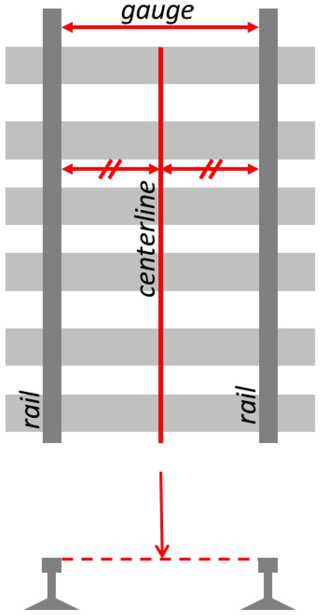
Figure 2.
Schematic presentation of centerline, gauge and rails.
MLS data delivers a dense description of the rail way environment, represented by hundreds or even thousands of 3D points per m2. Our method is designed to automatically reconstruct the position of the centerline using two approaches, as shown in Figure 3. They both start by detecting the points that hit the rail way tracks. The first is a data driven approach that calculates imaginary points in between points on two parallel rail tracks, followed by a curve fitting algorithm to get a smooth centerline. The second approach generates a 3D model of the rail tracks, taking into account parallelism and constraints to the smoothness and slope of rail way design. Based on the location of the 3D models, the centerline is implicitly defined as the line in the middle of the pair of rails.
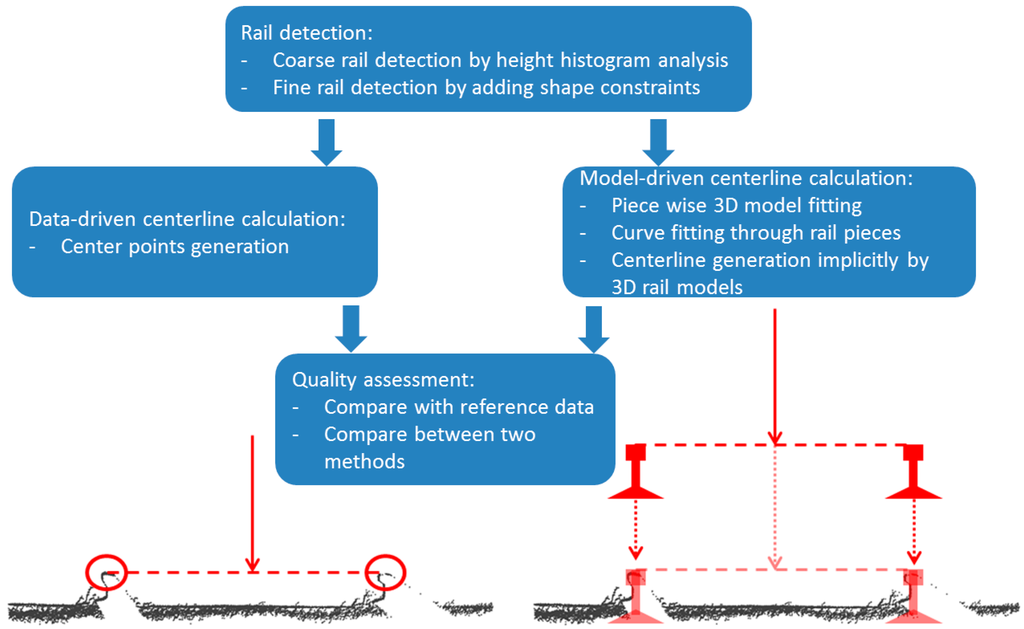
Figure 3.
Schematic workflow from rail detection to data-driven and model-driven centerline calculation.
3.2. Initial Rail Track Detection by Grid Wise Height Histogram Analyses
Generally, the rail track environment is an extremely standardized area, in terms of types and shapes of objects, open spaces, and distances between objects. This knowledge is integrated in the design of our method to detect and model rail tracks. For finding the majority of rail tracks, it can be assumed that the track itself is at or near the ground, that the space just above the tracks is empty, and that there may be contact wires and other wires at a certain height above the track. For detecting rail tracks in a mobile laser scanning point cloud, this can be implemented by checking whether these elements are presents in a certain area. We perform a coarse track detection by analyzing the height histogram of laser points in a 1 by 1 m neighborhood. In the lowest 0.5 m a search for points on a rail track is performed if the space above is rather empty. The height histogram analysis starts by taking the 10-th percentile point within each 1 × 1 m grid as DTM height. Next, if there are rails in this 1 square meter, there should be a rather empty space in between 0.5 and 4.5 m above this DTM height. If that is the case, then the terrain points are further analyzed by checking whether there are a few points that are slightly higher than the other terrain points. These points are initially classified as rail track points.
The result of this step is a coarse indication which points are at the rail track, based on the relative height to the ground and potential wires. There are situations where points may be either incorrectly detected as rail track (false positives) or not detected (false negatives). In order to remove false positives and to reduce the number of false negatives, we incorporate more shape knowledge of the rail track in the fine detection stage. A preliminary approach was described in [4]. One of the limitations of that approach was the implication of the RANdom Sample Consensus (RANSAC) line fitting approach which selects the best fitted line within a certain local neighborhood. As the neighborhood was defined by a regular grid of 1 × 1 m, only one rail track could be found within every m2: this meant that at switches part of the points on tracks were not selected. In this paper, we directly calculate point based features without the need to keep only the RANSAC inliers of a local fitted line. As a direct consequence, points on tracks near switches can still be detected automatically. As the point-based feature calculation is relatively expensive, the coarse track detection applied in this step helps reducing the computation time by eliminating the places where definitively no rail tracks are present.
3.3. Fine Rail Track Detection by Point Based Attribute Calculation
In this refinement stage, shape knowledge is used that a rail track locally is linear and two rails of a track are parallel. Therefore, we assume that points on rail tracks also show this pattern of linearity and parallelism. Per point the direction of nearby initially detected rail points is calculated, followed by an attribute that counts how many points are parallel at a given gauge distance.
For calculating the direction attribute for every coarsely detected rail point, nearby detected rail track points have been selected, e.g., within 1 m radius. Per point, the line is found iteratively such that most of the neighboring points is passing through that line within 3 cm distance. The line direction is taken as the direction attribute. Next, for every rail point we construct a parallel buffer at the gauge distance, and count the number of rail points that fall inside that buffer. Additional condition is that those points should have a similar direction value as well. If the number of points in the parallel buffer exceeds a threshold value, the point is classified as refined rail track point.
Due to the scanning configuration, it cannot be assumed that the points are symmetrically distributed over the tracks and over the rails per track. One side of a rail may be occluded for the scanner. This may have an influence on the determination of the centerline: the distribution of points may lean slightly towards the position of the scanner, causing that the centerline is not exactly in the middle of two point clouds of parallel tracks. Two different approaches are presented in 3.4 and 3.5 and aim to minimize the influence of this possibly asymmetric distribution of points.
3.4. Centerline Determination Directly from Detected Points
The data-driven approach selects only the top points of the detected tracks, assuming that the asymmetry in distribution is less systematic, even almost absent, at the top of the rail. For every point, the local direction of the track is known from the “direction” attribute, and it is known which points are at the parallel track within a certain radius. A line is fitted to points at the parallel track which contain the same direction value. Next, the perpendicular direction is determined and used to construct an across track line projected through the processed point. The midpoint of that projection is stored in a vector of center points, see Figure 4. The consequence is that for every detected rail track point one center point is generated, based on fitting a line through points at the parallel track. Additional property is that the center points are determined by parallel points with a distance of the gauge ±10 cm in-between the rail points. This means that even at switch locations center points have been determined by a pair of corresponding rail track pieces. The switch itself is recognized automatically as centerlines of one track will approach and even cross the rail track points of the track that joins or split from the first track. In our implementation, a minimum threshold of 0.6 m between center points and rail track points is used for single tracks, as by definition the distance should be around half the gauge distance, i.e., 0.70–0.75 m. If center points and rail tracks points are within 0.6 m, this can only mean a situation where the centerline is from another track than the track points, as shown in Figure 5.
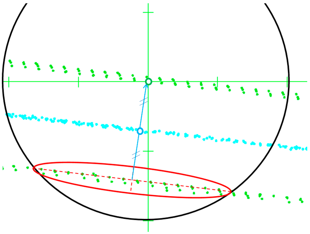
Figure 4.
Within a radius of 2 m (black circle), points are selected at the parallel track (red ellipse). The average direction of those points is used to construct a perpendicular line through the current rail track point (green dot). The center point is generated on that line (blue dot), exactly in between the rail track point and line through the selected parallel track points.
Next, points are grouped into segments. This holds for both the center points and the rail track points. The working of the segmentation is based on component growing algorithm using the maximum distances between points, constraining the point attributes of the local direction and their label, e.g., switch, left/right track and center points. Data gaps in along-track direction can be covered now that we can locally calculate the direction of the rail way. This enables us to group collinear segments. We limit the maximum data gap to cover to 8 m in track direction, in order to avoid possible incorrect grouping of different rail ways. At switch locations, our algorithm will stop the component growing as during the modeling stage we restrict to model parts in between two switches to reduce the degree of freedom. Rail track points and their corresponding center points at switch locations are grouped in a separate connected component. The result after this step is a labelled and segmented point cloud, where the segments correspond to groups of points on normal rail tracks, center points or switch points.
The generated center points have been used as input for an interpolation algorithm for our first approach to reconstruct the centerlines. Per rail track, all center points are collected and split into regular intervals, e.g., 2.0 m, along the rail track. For each interval one position is stored at the middle location of a straight RANSAC line fitted through the majority of points in that interval. If an interval appears to have no center points due to a local data gap, center points are interpolated at a straight line from the previous known center location until the next interval after the gap. The second approach for center line reconstruction, discussed in the next section, is based on 3D rail track modeling, making use of the detected rail track points and a parametric track model.
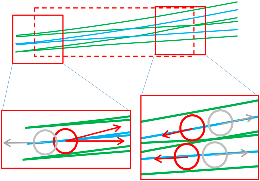
Figure 5.
Switch detection (dashed red box) by checking distances between rail track points and center points. Red circles indicate locations where rail track points are closer than e.g., 60 cm to the center points. Grey circles indicate normal situations where center points and track points are more than 60 cm apart.
3.5. Centerline Determination by 3D Modeling of the Rail Tracks
The model-driven approach calculates 3D models by fitting parametric track models to the detected rail track points. For this approach not only the top of the track is considered but also the foot of the track. For this, all points directly below the detected rail top are included in the detected rail track data as well. The 3D rail model is generated by fitting parametric pieces to point segments along the rail, followed by interpolating a smooth and continuous rail model between the pieces. The following sections describe the steps in this process.
3.5.1. Defining a Parametric Model of a Rail Piece
The parametric model consists of a pair of two simplified rail pieces, as shown in Figure 6. It is defined by eight shape parameters and six orientation parameters. The shape parameters are considered fixed throughout the track, and are obtained from standard railway specifications. The orientation parameters define the position and rotations of the local coordinate system of the model with respect to the global coordinate system of the point cloud, and are estimated for each piece. Compared to our previous model [4], where the left and the right rail were modelled independently, the current model allows modeling both rails simultaneously. This guarantees that the left and right pieces always have the same orientation, and that the final model has a constant gauge distance throughout the rail track.
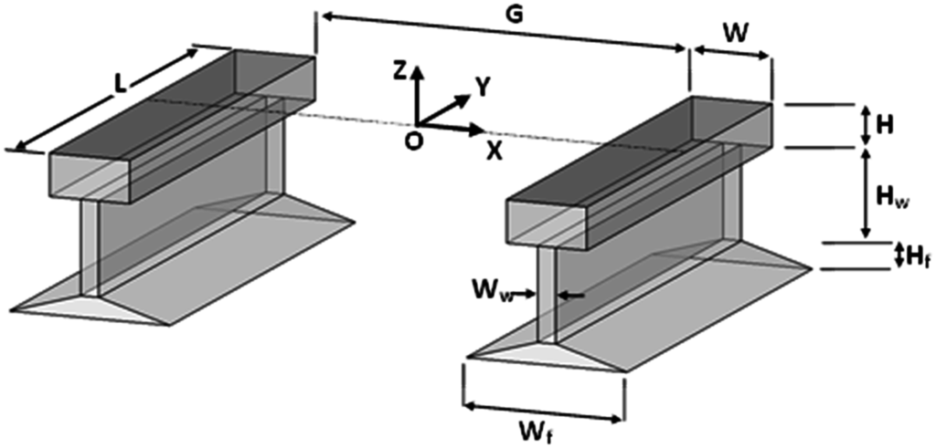
Figure 6.
Parametric model of a pair of two rail pieces. Position and the orientation parameters of the local coordinate system need to be determined.
3.5.2. Estimating the Parameters of a Piece Model
To fit the parametric pieces to the points, first the points detected on both rails are partitioned into small segments of size L (length of the model) along the main axis of the track. For this purpose, the center points generated in the previous step are used as the approximate axis of the track.
The common approach to parametric model fitting is by least-squares estimation of the model parameters, minimizing a measure of distance between the model and the data [19,20]. However, the least-squares estimation method is largely influenced by the missing points and outliers, which are difficult to avoid in the detection step. For this reason, we adopt a Markov Chain Monte Carlo (MCMC) algorithm to estimate the parameters of each piece by sampling the joint probability distribution of the orientation parameters. Formally, for a given set of points Xj in segment j, the aim is to find a model Ɵj that maximizes the probability p(Ɵj|Xj), where Ɵj = [xoj, yoj, zoj, ωj, ϕj, κj]T is the vector of six orientation parameters of the model. Using Bayes’ rule:
where p(Xj|Ɵj) is the evidence for the model provided by the points, p(Ɵj) is the model prior, and is a normalization factor that does not affect the choice of Ɵj. We define the evidence as:
where is the mean distance between the points in segment j and the model Ɵj , and c is a constant. The point-model distance is defined as the perpendicular distance from a point to its corresponding planar patch in the model. To find the corresponding patch, the point is orthogonally projected to each of the patches of the model, and the projected point is tested whether it is contained within the boundary of the patch. The patch that contains the orthogonal projection of the point is selected as the corresponding patch, and its perpendicular distance from the point is calculated. Points that do not project to any of the patches (these are usually points that are far away from the model) are excluded from the calculation of in Equation (2).
p(Ɵj|Xj) = ηp(Xj|Ɵj)p(Ɵj)
The prior p(Ɵj) is used to incorporate our prior knowledge of the model parameters. We expect that the rotation parameters of each rail piece are only slightly different from the previous piece, and that the position of a piece is close to the center of its corresponding point segment. To include this knowledge, we define the prior as a normal distribution centered around the expected rotation and position parameters of the piece model:
where µj is the mean vector and ∑j is the covariance of the parameters in Ɵj. The mean vector contains the expected rotation (i.e., the rotation of the previous piece) and position (i.e., the center of the point segment) of the piece. For the first piece in each track we set ω1 = 0 and ϕ1 = 0, while κ is obtained as the direction of the approximate centerline. The covariance of the prior distribution ∑j is defined by assuming large variances for the expected orientation parameters and no correlation between them. The large variances ensure that the Markov chain does not get stuck at the mean of the prior distribution.
p(Ɵj) ~ N(µj, ∑j)
For the MCMC sampling the Metropolis-Hastings algorithm [21] is used. The algorithm starts at a random initial point and recursively provides samples Ɵt, t = 1,…,n from the target distribution p(Ɵj|Xj). The samples are drawn from a proposal distribution, which is chosen as a Gaussian with variances larger than the prior distribution. An estimate of the expectation of model parameters is then obtained by the ergodic mean of the samples: , where m specifies the number of so-called burn-in samples. Further details about the Metropolis-Hastings algorithm can be found in [22].
3.5.3. Interpolating a Smooth and Continuous Rail Model
The rail pieces obtained by the MCMC sampling do not necessarily form a continuous and smooth rail track. The estimated orientation parameters are defined at the local origins (of the coordinate systems of the pieces) at intervals of approximately L (length of a piece). To obtain a continuous and smooth model of the rail tracks, the orientation parameters should be interpolated in between these local origins. As rail tracks typically consist of straight segments and circular curves, we choose a Fourier series as the interpolation function:
where Ɵi(t), i = 1,..,6 is i-th orientation parameter at an intermediate location t in the interval [1, m], m being the number of rail pieces, ak, bk, w are the unknown coefficients of the interpolation function and n is its order. The interpolation coefficients are estimated for each parameter separately. By evaluating Equation (4) with the known Ɵi of all pieces, a system of equations is obtained, which is then solved for the unknown coefficients. The estimated coefficients minimize the sum of squared differences between the piece parameter and the interpolated value. The order of the Fourier series defines the flexibility of the fitted curve. However, higher order Fourier series may result in oscillation and waviness in the final model. By experiment we found that the third order Fourier series is sufficient to fit a smooth curve to the orientation parameters accurately.
Once the interpolation coefficients are estimated for each orientation parameter, we can reconstruct a continuous and smooth model of the rail track by connecting very small rail pieces using the interpolated orientation parameters. The centerline of the reconstructed rail track is simply obtained as the set of interpolated position parameters along the rail track.
4. Results
4.1. Dataset Description
To evaluate the methods, MLS data were acquired in two study areas. The first dataset was acquired at the Blerick train station near Venlo, and the second dataset was acquired at the train station of Sittard, both cities located in the south of the Netherlands. In Figure 7, laser data of two areas are shown. The data has been captured by Fugro using the RAIL-MAP system. This system contains a GNSS/INS system, a panoramic camera and two laser scanners. The system is dedicated and certified for use on railways. It can be mounted on a train and operate at regular track speeds, such that the train schedule will not be disrupted. The scanners are based on the measurement of phase shift. Each scanner is capable of registering up to 1 million points per second. Both scanners send the laser wave in a slightly inclined plane to reduce shadowing effects. The range accuracy is in the order of 1–3 mm, whereas the positional accuracy of the system as a whole is in the order of 1 cm. All areas contain several parallel rail tracks. Green arrows indicate the tracks at which the system has acquired the data. In Figure 7 area “Blerick” is shown, containing at least 6 parallel rail tracks where the system was mounted on a vehicle on the rightmost rail track. The rightmost track is at an across distance of between 25 and 30 m from the left track. One switch is located in the right part of this dataset. This size of the area is 350 × 40 m, containing 5.8 Million points. In Figure 7 the dataset of “Sittard”, 600 × 80 m containing about 25 Million points, is shown with 9 parallel rail tracks on which on two of the tracks the MMS-vehicle has driven to acquire data.
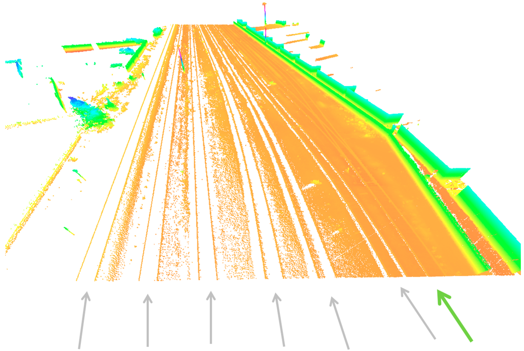
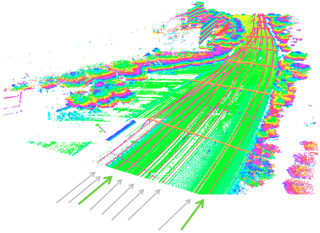
Figure 7.
Point cloud from area near station Blerick (top) and Sittard (bottom). Data has been acquired on tracks indicated by the green arrows.
Reference data has been used for testing the positional accuracy of the extracted centerlines. This reference data has been captured by Fugro with the RiLa system. This is a system carrier two laser scanners recording only the tracks directly below the sensor (RiLa, 2015), determining track geometry with an absolute accuracy of 1.5 cm. For the reference data of Sittard it was known at forehand that some of the reference centerlines would have an unknown systematic offset of a few centimeters. For Sittard we therefore calculate and eliminate the systematic error per rail track and focus on the standard deviation to the reference data.
4.2. Rail Track Detection
In Figure 8, part of the Blerick area is shown where points in green are roughly classified as rail track points. The points colored by segment in the lower figure are the refined rail track classification results. It can be seen that all of the false positives (indicated by red arrows) have been removed in the refinement step. The downside of this strict removal is that also some of the true positives are removed when the results become uncertain. This can be seen on the fourth parallel track, highlighted in the red ellipse. Three of the parallel tracks can be identified, plus the track where the system was driving. On the fourth parallel track, classification results become noisier and the refined classification step is not able to reliably detect points anymore. The reason is that we assume the rails are slightly elevated above the ground whereas on those rails there are no points on the ground; therefore rail points have not been detected. The parallel rail track can never be found in this case, when points from one of the two parallel rails have not been extracted in the rough classification. Although this may be a limitation of our algorithm, it is not considered to be a practical problem. In practice there will be enough possibilities to capture data on at least one of the other rail tracks instead of only the outer left one. An alternative solution is to integrate Airborne Laser Scanning (ALS) data to the MLS data to get the position of the terrain at the occluded areas in the MLS data. Once the terrain height is known from the ALS data, the detailed position of the rail tracks will come from the MLS points on the rail track.
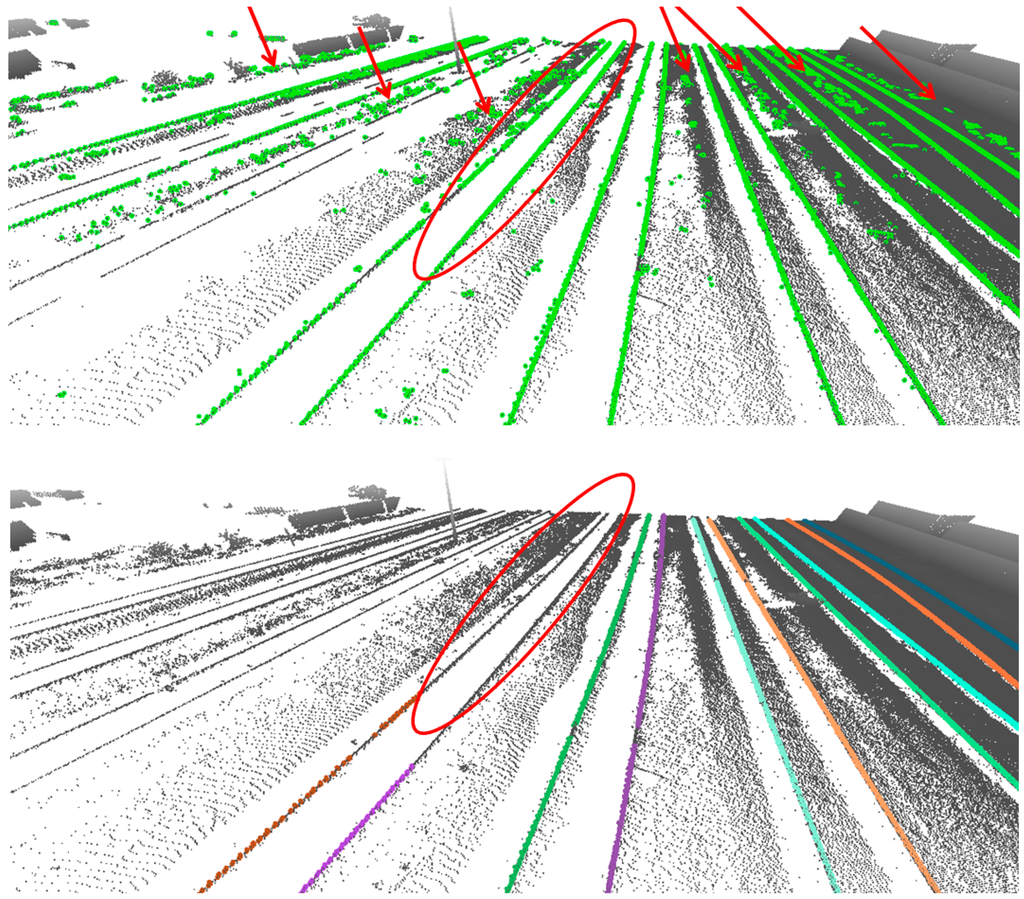
Figure 8.
Coarse (top) and fine (bottom) rail track detection in Blerick. MLS data has been captured at the most right rail track.
In the following figures, results of track detection and center line generation are shown. The upper row views of Figure 9 are constructed by an orthogonal projection of the points to a tilted plane, the bottom row are perspective views on a part of the data. It can be seen in the bottom row that center points can be generated even at locations where no rail points were detected on a path crossing the rail tracks.
Our second approach models 3D rail tracks by piece-wise fitting of parametric models followed by interpolation. The origins of the fitted pieces are the locations of the center lines. As a side-result, the 3D models are also generated. Results of the models are shown in Figure 10, together with the original point cloud and the locations of the generated center points. Rail models are represented by a wireframe model. Positions and orientations of the rail models are determined every 20 cm along the curve. Therefore, also the center points have been generated at intervals of 20 cm.
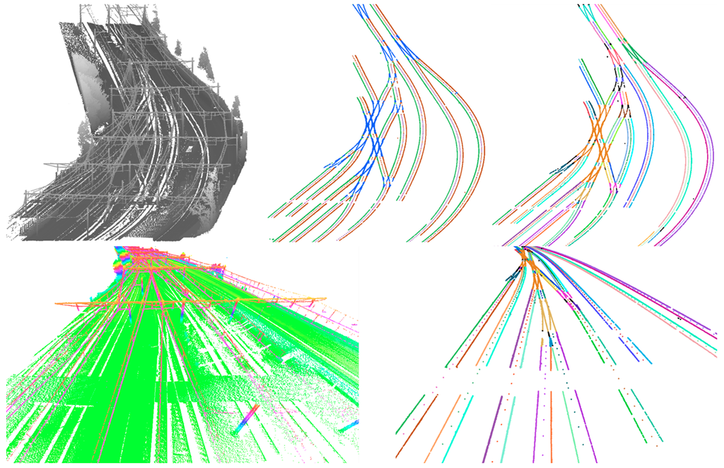
Figure 9.
Rail track detection and centerline extraction from Sittard area. Top and bottom left: original point cloud; top center: points labelled by left/right rail piece, center points and switches; top and bottom right: points colored by connected component, center points derived at intervals of 2 m.
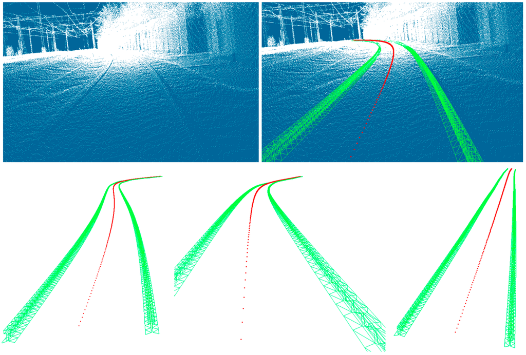
Figure 10.
3D Models and centerlines overlaid on raw point cloud data.
4.3. Accuracy Analysis of Center Line Extraction
Each generated center point is perpendicularly projected onto the corresponding reference centerline. In order to analyze whether potential discrepancies have a stochastic or systematic appearance, the signed distance has been calculated. Per rail track we analyze the behavior of the residuals between generated and reference center lines, by calculating the root means square error (RMSE), the bias and standard deviation per track. This is done for both the data-driven approach and the model-driven approach, i.e., after rail track fitting. The reference data itself has an expected standard deviation of 1.5 cm per center point. For both of our approaches the results are visualized in Figure 11.
Point colors indicate the magnitude of the residuals at the generated center points. Grey lines represent the direction and magnitude of the residuals between generated center points and the corresponding reference centerline. The length of the lines is magnified by a factor 20 to enhance the interpretation of the figures.

Figure 11.
Residuals between generated centerlines and reference data for our data-driven approach (left) and the model-driven approach (right) in Blerick. Grey lines represent the direction and magnitude of the residuals (magnified by a factor 20).
Analysis of the behavior of the residuals in done in two directions:
- -
- Along track direction; to analyze systematic patterns caused by curve fitting in our second approach and/or curve fitting in the reference data.
- -
- Across track direction; to analyze the capability to generate center lines at parallel rail tracks next to the current rail track. Both systematic and stochastic errors are analyzed. The scanning angle may cause systematic effects for parallel tracks far away, and the decreasing point density may result in higher standard deviation values.
In along track direction one may see a small systematic pattern at the most right line, just after the curve for both methods in Figure 11. This is the lane where the system was driving. Residuals are between 2 and 3 cm at those locations, at other check points residuals are below 2 cm. The standard deviation of all residuals per track is listed in the figure varying from 1.0 to 2 cm. Note that in these values the effects of noise in the reference data is also included, meaning that both approaches have a standard deviation of better than 2 cm. In other words, the geometric quality of our results is comparable to the quality of the reference data.
In across track direction it can be seen that the standard deviation is increasing from 1.2 to 1.6 cm for approach 1 and 1.3–2 cm for approach 2 when moving further away from the sensor position. Although the pattern is not that strong, it is still arguable that the standard deviation increases from right to left. The bias does not show a clear pattern in across track direction. This means that our method is capable of generating centerlines at parallel tracks, with a slight decrease of precision for decreasing point densities.
For Sittard, the standard deviation of the residuals between reference data and generated center lines ranges from 1.3 to 2.7 cm, see Figure 12. The systematic offset (italic values in the figure) varies up to 5 cm per track. This can be caused by offsets in the reference data which have been produced on a track-wise base, or misalignments in the MLS system between position sensors and ranging sensors or a combination of these two causes. For Fugro this has been a reason to further analyze the chain of measurements in both the MLS system and the reference measurements to reduce the influence of potential systematic errors.
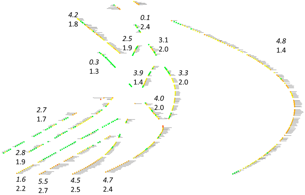
Figure 12.
Residuals between centerlines from data-driven approach and reference data in Sittard: top value is the systematic offset, bottom value represent the standard deviation of the residuals per track. Grey lines represent the direction and magnitude of the residuals (magnified by a factor 20).
The influence of the modeling and Fourier series interpolation function is checked by comparing the center lines from the data-driven approach with the ones after 3D modeling and curve fitting. As the detected rail points are the same for both approaches, differences can only be explained by differences in the further processing steps. Differences are shown in Figure 13, where the maximum difference occurs at the most curved area in the datasets. The geometric differences of the center line location between the two approaches is mostly below 1 cm but can reach up to 2.7 cm in curved situations. This is a direct consequence of the use of the curve fitting algorithm, and how well the fitted curve fits to the rail track.
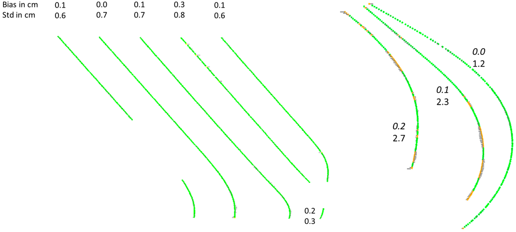
Figure 13.
Differences between data-driven and model-driven approach in Blerick (left) and Sittard (right).
5. Conclusions
The fact that a pair of rail tracks is parallel and locally linear are the most essential properties that have been used in the rail track and center points’ determination. These properties reduce the number of initially false detected rail points from the rough detection stage. Our approach can deal with local data gaps, as the scene constraints of rail way tracks are strong enough to bridge several meters without data. In cases of data gaps longer than 8 m at the rail track or its supporting ground surface, our algorithm cannot recognize connections between detected rail segments. In practice, it resulted in the correct reconstruction of four neighboring rail tracks, where the fifth contains too many data gaps due to self-occlusion by the rail track.
The aim of this research was to analyze whether we can accurately and automatically determine centerlines of rail tracks, even if the platform is at another rail track. We have shown that it is indeed possible to generate centerlines as long as rail tracks can be identified. Two approaches have been presented in this paper: the first determines the center position directly between points of a pair of rails. The second approach models the rail track by fitting a parametric model to the extracted rail points.
Both of our approaches prove that the geometric accuracy of the extracted centerlines is between 1 and 3 cm. The geometric differences of the center line location between the two approaches is mostly below 1 cm but can reach up to 2.7 cm in curved situations.
The geometric quality of the reference data is comparable with the quality of our results. Although this makes it challengeable to draw hard conclusions on the exact accuracy of our method, it proves that our approach is a very attractive alternative knowing that it is based on a fully automated procedure.
Future work includes automated extraction and modeling of other objects in a railway environment such as the platforms, catenary wires and towers. Next, existing 2D geo-information for the rail tracks will be updated and converted into 3D.
Acknowledgments
The authors would like to deeply thank Martin Kodde and Rikkert Wienia from Fugro GeoServices not only for providing RAIL-MAP data and reference data, but also for their valuable input on the working of the systems and the practical importance of this method.
Author Contributions
Next to the overall paper writing and organization, Sander Oude Elberink designed the method for rail point classification and data-driven center points generation. Kourosh Khoshelham performed the parametric modeling and curve fitting for the model-driven centerline extraction.
Conflicts of Interest
The authors declare no conflict of interest.
References
- Petrie, G. Mobile mapping systems: An introduction to the technology. GeoInformatics 2010, 13, 32–43. [Google Scholar]
- Puente, I.; González-Jorge, H.; Martínez-Sánchez, J.; Arias, P. Review of mobile mapping and surveying technologies. Measurement 2013, 46, 2127–2145. [Google Scholar] [CrossRef]
- Vaaja, M.; Kukko, A.; Kaartinen, H.; Kurkela, M.; Kasvi, E.; Flener, C.; Hyyppä, H.; Hyyppä, J.; Järvelä, J.; Alho, P.; et al. Data processing and quality evaluation of a boat-based mobile laser scanning system. Sensors 2013, 13, 12497–12515. [Google Scholar] [CrossRef] [PubMed]
- Oude Elberink, S.; Khoshelham, K.; Arastounia, M.; Díaz Benito, D. Rail track detection and modelling in mobile laser scanner data. ISPRS Ann. Photogramm. Remote Sens. Spat. Inf. Sci. 2013, 1, 223–228. [Google Scholar] [CrossRef]
- Kaleli, F.; Akgul, Y.S. Vision-based railroad track extraction using dynamic programming. In Proceedings of the 2009 IEEE 12th International Conference on Intelligent Transportation Systems, St. Louis, MO, USA, 4–7 October 2009; pp. 1–6.
- Zhu, L.; Hyyppa, J. The use of airborne and mobile laser scanning for modeling railway environments in 3D. Remote Sens. 2014, 6, 3075–3100. [Google Scholar] [CrossRef]
- Beger, R.; Gedrange, C.; Hecht, R.; Neubert, M. Data fusion of extremely high resolution aerial imagery and lidar data for automated railroad centre line reconstruction. ISPRS J. Photogramm. Remote Sens. 2011, 66, S40–S51. [Google Scholar] [CrossRef]
- Neubert, M.; Hecht, R.; Gedrange, C.; Trommler, M.; Herold, H.; Krüger, T. Extraction of railroad objects from very high resolution helicopterborne lidar and ortho-image data. Int. Arch. Photogramm. Remote Sens. Spat. Inf. Sci. 2008, 38, 25–30. [Google Scholar]
- Yang, B.; Fang, L. Automated extraction of 3-d railway tracks from mobile laser scanning point clouds. IEEE J. Sel. Top. Appl. Earth Obs. Remote Sens. 2014, 7, 4750–4761. [Google Scholar] [CrossRef]
- Tang, P.; Huber, D.; Akinci, B.; Lipman, R.; Lytle, A. Automatic reconstruction of as-built building information models from laser-scanned point clouds: A review of related techniques. Autom. Constr. 2010, 19, 829–843. [Google Scholar] [CrossRef]
- Maas, H.-G.; Vosselman, G. Two algorithms for extracting building models from raw laser altimetry data. ISPRS J. Photogramm. Remote Sens. 1999, 54, 153–163. [Google Scholar] [CrossRef]
- Verma, V.; Kumar, R.; Hsu, S. 3D building detection and modeling from aerial lidar data. In Proceedings of the 2006 IEEE Computer Society Conference on Computer Vision and Pattern Recognition, New York, NY, USA, 17–22 June 2006; pp. 2213–2220.
- Rabbani, T.; Heuvel, F.V.D. Methods for fitting CSG models to point clouds and their comparison. In Proceedings of the 7th IASTED International Conference on Computer Graphics and Imaging, Kauai, HI, USA, 17–19 August 2004; pp. 279–284.
- Lai, K.; Fox, D. Object recognition in 3d point clouds using web data and domain adaptation. Int. J. Robot. Res. 2010, 29, 1019–1037. [Google Scholar] [CrossRef]
- Diaz Benito, D. Automatic 3d Modelling of Train Rails in a Lidar Point Cloud. M.Sc. Thesis, University of Twente, Enschede, The Netherlands, 2012. [Google Scholar]
- Miao, Z.; Wang, B.; Shi, W.; Wu, H. A method for accurate road centerline extraction from a classified image. IEEE J. Sel. Top. Appl. Earth Obs. Remote Sens. 2014, 7, 4762–4771. [Google Scholar] [CrossRef]
- Miao, Z.; Shi, W.; Zhang, H.; Wang, X. Road centerline extraction from high-resolution imagery based on shape features and multivariate adaptive regression splines. IEEE Geosci. Remote Sens. Lett. 2013, 10, 583–587. [Google Scholar] [CrossRef]
- Soni, A.; Robson, S.; Gleeson, B. Extracting rail track geometry from static terrestrail laser scans for monitoring purposes. Int. Arch. Photogramm. Remote Sens. Spat. Inf. Sci. 2014, XL-5, 553–557. [Google Scholar] [CrossRef]
- Lowe, D.G. Three-dimensional object recognition from single two-dimensional images. AI 1987, 31, 355–395. [Google Scholar]
- Khoshelham, K.; Li, Z.L. A model-based approach to semi-automated reconstruction of buildings from aerial images. Photogramm. Rec. 2004, 19, 342–359. [Google Scholar] [CrossRef]
- Hastings, W.K. Monte carlo sampling methods using markov chains and their applications. Biometrika 1970, 57, 97–109. [Google Scholar] [CrossRef]
- Gilks, W.R.; Richardson, S.; Spiegelhalter, D. Markov Chain Monte Carlo in Practice; Chapman and Hall/CRC: Boca Raton, FL, USA, 1995. [Google Scholar]
© 2015 by the authors; licensee MDPI, Basel, Switzerland. This article is an open access article distributed under the terms and conditions of the Creative Commons Attribution license (http://creativecommons.org/licenses/by/4.0/).