Article

Polarimetric Calibration of CASMSAR P-Band Data Affected by Terrain Slopes Using a Dual-Band Data Fusion Technique

1
The State Key Laboratory of Information Engineering in Surveying, Mapping and Remote Sensing (LIESMARS), Wuhan University, Wuhan 430079, China
2
School of Environmental Science and Spatial Informatics, China University of Mining & Technology, Xuzhou 221008, China
*
Author to whom correspondence should be addressed.
Remote Sens. 2015, 7(4), 4784-4803; https://doi.org/10.3390/rs70404784
Submission received: 22 December 2014 / Revised: 13 April 2015 / Accepted: 14 April 2015 / Published: 20 April 2015
(This article belongs to the Special Issue Remote Sensing Dedicated to Geographical Conditions Monitoring)

Abstract

:
For airborne synthetic aperture radar (SAR) polarimetric calibration (PolCAL) based on distributed targets, it is important to ensure the removal of both the polarimetric distortion and terrain slope effect. This paper proposes a new technique for PolCAL in mountainous areas, without the use of corner reflectors (CRs). The technique based on dual-band data fusion consists of two steps. First, the polarization orientation angle shift (POAS), as a priori asymmetry information, is derived from X-band interferometry and applied to P-band fully-polarimetric data. Second, the crosstalk and cross-polarization (cross-pol) channel imbalance are iteratively determined using the POAS after dual-band data fusion. The performance and feasibility of the technique was evaluated by CRs. It was demonstrated that the proposed technique is capable of deriving the distortion parameters and performs better than the methods presented in Quegan and Ainsworth et al. The signal-to-noise ratio (SNR) and pedestal height have been investigated in polarimetric signatures. The proposed technique is useful for PolCAL in mountainous areas and for monitoring systems without CRs in long-term operation.

Graphical Abstract

1. Introduction

Fully-polarimetric SAR data are useful for understanding the polarization reflection properties of observed objects in many applications, such as geographical condition monitoring and environmental change study. In order to further utilize fully-polarimetric data, polarimetric calibration (PolCAL), which focuses on the removal of the radar antenna system distortion effect, is a fundamental pre-processing step [1]. PolCAL has two different applications in both the short and long term. The short-term application is to estimate the system distortion parameters for converting un-calibrated data to calibrated data. The long-term application is to monitor the radar antenna system distortion and to prevent undesirable effects. In either case, it is necessary to rely on distributed targets or point targets in the calibration site. Distributed targets in the calibration site should meet scattering reciprocity and reflection symmetry assumptions [2,3,4,5], such as the Amazon rainforest over flat terrain [6,7,8,9]. In addition, calibration can also be achieved by deploying one or more corner reflectors (CRs) as point targets [10,11,12,13,14] in the calibration site. For extensive and long-term SAR data acquisition, both spaceborne SAR and airborne SAR systems, such as PALSAR and Pi-SAR [15,16,17,18,19], should undertake PolCAL constantly.
The Chinese Academy of Surveying and Mapping Synthetic Aperture Radar (CASMSAR) system, which is China’s first airborne SAR mapping system, was developed in 2009 [20,21]. The system is normally operated with dual-band high-resolution SAR sensors, single-pass cross-track interferometry in the X-band and concurrent fully-polarimetric (quad-polarization) measurement in the P-band (Figure 1a), and its main parameters are shown in Table 1. CASMSAR has operated more than 200 flights in China since 2009. Most of the flights were conducted in mountainous areas of western China, where deploying CRs is difficult due to the rugged terrain [22,23,24,25]. In such terrain, relying on distributed targets becomes a practical choice for PolCAL. However, terrain slopes and aspects in mountainous areas can result in distributed target reflection asymmetry. The asymmetry is usually caused by terrain slopes and aspects in airborne SAR acquisition and by terrain slopes and aspects and Faraday rotation in spaceborne SAR acquisition [26,27,28]. Recently, several new PolCAL methods based on distributed targets have been proposed to solve the asymmetry problem. Ainsworth et al. [29] used an a posteriori calibration method to preserve the orientation angle of asymmetric targets. Kimura et al. [30] proposed a method to remove the Faraday rotation effect for calibration by the use of a priori information about the polarization orientation angles of built-up areas in the calibration site.
A new technique for PolCAL using a priori asymmetry information of distributed targets from the dual-band data fusion is proposed and evaluated in this paper. The rest of the paper is organized as follows. In Section 2, the calibration model based on distributed targets is determined by adding the polarization orientation angle shift (POAS). The method used to derive the a priori POAS is introduced in Section 3. The method used to estimate the distortion parameters is also presented. In Section 4, the proposed PolCAL scheme and some practical details are presented. In Section 5, the performance of the proposed PolCAL technique is analyzed and validated by comparison with results from deployed CRs (see Figure 1b), and the experimental results with four datasets are presented. Finally, Section 6 gives the conclusions.
Figure 1. (a) Antennas mounted under the aircraft body; (b) Corner reflector deployed in the calibration site.
Remotesensing 07 04784 g001
Table 1. The main parameters of the CASMSAR system.
FrequencyPolarizationBaselineGround ResolutionIncidence Angle
X9.6 GHzHH2.198 m0.5/1.0/2.5/5.0 m37°–63°
P600 MHzHH, HV, VH, VVN/A1.0/2.5/5.0 m33°–53°

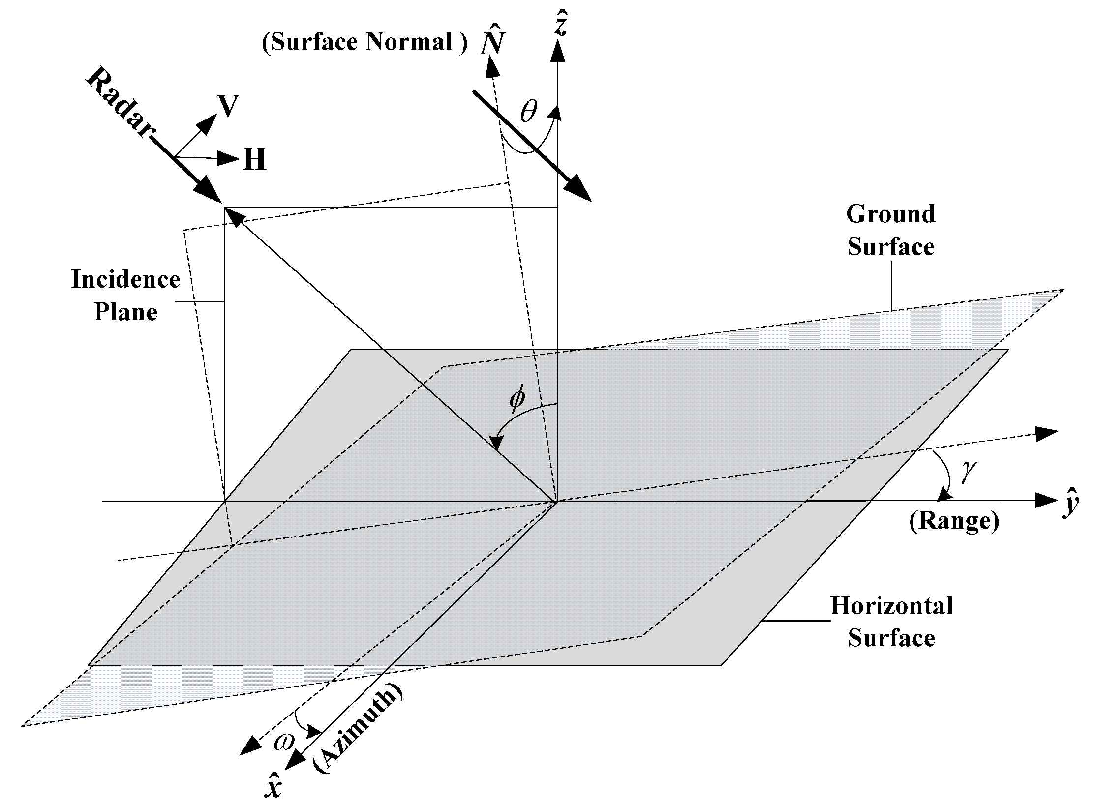
2. Polarimetric Distortion Affected by Reflection Asymmetry

True measurements of backscatter are distorted by polarimetric transformation errors (crosstalk and channel imbalance) on reception and transmission, in addition to additive system noise. The relationship between the observed scattering matrix O and the true scattering matrix S can be expressed by the following equation:
O = R S T + N
where R is the received distortion matrix, T is the transmitted distortion matrix and N is the system noise matrix. According to [29], the matrices in Equation (1) are all 2 × 2 complex matrices. Without the consideration of the noise contribution, Equation (1) is equivalent to:
[ O HH O HV O VH O VV ] = [ r HH r HV r VH r VV ] [ Z HH Z HV Z VH Z VV ] [ t HH t HV t VH t VV ]
where Z is equal to scattering matrix S of (1) without rotation and subscripts H and V refer to the horizontal and vertical polarization states. If true measurements of backscattering are affected by terrain slopes and aspects, the measured scattering matrix after rotation is:
[ Z HH Z HV Z VH Z VV ] = [ cos θ sin θ sin θ cos θ ] [ S HH S HV S VH S VV ] [ cos θ sin θ sin θ cos θ ]
where Z denotes scattering matrix S after rotation by θ and θ is the POAS. Combining Equation (2) and Equation (3), one obtains:
[ O HH O HV O VH O VV ] = [ r HH r HV r VH r VV ] [ Z HH Z HV Z VH Z VV ] [ t HH t HV t VH t VV ] = [ r HH r HV r VH r VV ] [ cos θ sin θ sin θ cos θ ] [ S HH S HV S VH S VV ] [ cos θ sin θ sin θ cos θ ] [ t HH t HV t VH t VV ] .
Quegan and Ainsworth converted these scattering matrices (O, S) to vector format [29], According to [29], one can rewrite (4) as:
[ O HH O HV O VH O VV ] = ( t VV r VV ) [ k 2 a v k w k a v w z k 2 a k w z k a w u k 2 a u v k k a v u z k 2 a u k z k a 1 ] [ Z HH Z HV Z VH Z VV ] = ( t VV r VV ) [ M ] [ Z HH Z HV Z VH Z VV ] = ( t VV r VV ) [ M ] [ cos 2 θ sin θ cos θ sin θ cos θ sin 2 θ sin θ cos θ cos 2 θ sin 2 θ sin θ cos θ sin θ cos θ sin 2 θ cos 2 θ sin θ cos θ sin 2 θ sin θ cos θ sin θ cos θ cos 2 θ ] [ S HH S HV S VH S VV ] = ( t VV r VV ) [ k 2 a v k w k a v w z k 2 a k w z k a w u k 2 a u v k k a v u z k 2 a u k z k a 1 ] [ cos 2 θ sin θ cos θ sin θ cos θ sin 2 θ sin θ cos θ cos 2 θ sin 2 θ sin θ cos θ sin θ cos θ sin 2 θ cos 2 θ sin θ cos θ sin 2 θ sin θ cos θ sin θ cos θ cos 2 θ ] [ S HH S HV S VH S VV ] .
Equation (5) can be written in the form:
O = Y M P S
where u, v, w, and z are the four crosstalk components, the values of k and α characterize the co-pol and cross-pol channel imbalance, Y is the absolute calibration factor, M is the antenna distortion matrix, and P is the polarization orientation angle distortion matrix. The corresponding definitions in terms of the received and transmitted matrix are as follows: Y = tVVrVV, k = rHH/rVV, α = rVVtHH/rHHtVV, u = rVH/rHH, v = tVH/tVV, w = rHV/rVV, z = tHV/tHH.

3. Polarimetric Calibration Using the POAS

3.1. Deriving an a priori POAS

θ is geometrically related to the topographical slopes and the radar look angle [31]. A schematic diagram about θ is given in Figure 2. For a horizontal surface, its surface normal N ^ is in the incidence plane ( y ^ , z ^ ), and the orientation angle is not shifted. However, for a tilt ground surface, its surface normal is out of the incidence plane. θ is the angle that rotates the incidence plane about the line of sight for return to the surface normal. According to [31], θ due to the topographical slope effect can be expressed as:
tan θ = tan ω tan γ cos ϕ + sin ϕ
where tan ω is the azimuth slope, tan γ is the slope in the ground range direction and ϕ is the radar look angle. This equation shows that the orientation angle shift is mainly induced by the azimuth slope and is also a function of the range slope and the radar look angle. For an estimation of θ, three parameters are required. Due to the concurrent X-band operation in CASMSAR, θ can be calculated by the use of a digital elevation model (DEM) derived from X-band SAR interferometry.
Figure 2. Schematic diagram of inducing θ in the geometry.
Remotesensing 07 04784 g002

3.2. Derivation of the Calibration Model

For the a posteriori calibration model, Ainsworth made the first attempt to construct it for preserving orientation angle information. To construct the a priori model, combining [29] and [31], the covariance matrix can be obtained from the observed scattering matrix O conjugate multiplication. The covariance matrix can be expressed as:
C = O O H = Y M P S ( S P M Y ) H = ( Y X F K P ) E ( P K F X Y ) H
With X = [1 v w vw; z 1 wz w; u uv 1 v; uz u z 1], F = diag (α, 1, α, 1), K = diag (k2, k, k, 1).
To construct non-linear equations for expressing the calibration problem, a new equation can be obtained by inverting Equation (8) and dropping the absolute calibration factor Y due to the absolute radiometric calibration being irrelevant to PolCAL. It can be expressed as:
E ( P M ) 1 C ( ( M P ) H ) 1 = ( P K F X ) 1 C ( ( X F K P ) H ) 1
where superscript H represents the transpose and conjugate, X is the crosstalk matrix and E is the true covariance matrix. F and K are the matrices of the cross-pol and the co-pol channel imbalance, respectively. Most of the well-known PolCAL methods depending on the a priori information of distributed targets pose two kinds of assumptions:
(1)
Reciprocity SHV = SVH, which is the distributed targets’ constant physical property for a monostatic system.
(2)
Reflection symmetry 〈Sij×Sji〉= 0, which implies that the true co-pol and cross-pol returns are uncorrelated, unless the target’s orientation angle is changed.
Based on the above-mentioned assumptions, the assumed cases can be converted to the corresponding components of the true covariance matrix. The assumed true covariance matrix is:
E = [ E HHHH E HHHV E HHVH E HHVV E HVHH E HVHV E HVVH E HVVV E VHHH E VHHV E VHVH E VHVV E VVHH E VVHV E VVVH E VVVV ] = [ E HHHH 0 0 E HHVV 0 G G   0 0 G   G 0 E VVHH 0 0 E VVVV ]
where superscript * is the conjugate symbol, G shows that HV and VH are identical and the eight elements of zeroes of the covariance matrix E imply the reflection symmetry.

3.3. The Crosstalk and Cross-Pol Channel Imbalance Estimation

By inserting Equation (10) into Equation (9), it is then possible to derive eight equations from the eight zero elements of the covariance matrix E. Due to the covariance matrix E being a Hermitian conjugate matrix, we can only select four elements to construct non-linear equations. If expanding all of the terms, 256 items will be expressed in every equation, such as:
E HVHH = [ E ] ( r o w 1 , c o l 2 ) = [ P 1 M 1 C ( M T ) 1 ( P T ) 1 ] ( r o w 1 , c o l 2 ) = ( sin 2 θ sin 2 θ ( C VHVH constant term + u C HHVH + v C VVVH + u C VHHH + v C VHVV first order + u v C HVHH + second order and higher ) / 2 16 terms + sin 2 2 θ (- C HHVH + ) / 4 + 15 × 16 terms 16 × 16 = 256 terms   ) / Δ HVHH D HVHH / Δ HVHH  =  0 E HVVV  = D HVVV / Δ HVVV 0 E VHHH  = D VHHH / Δ VHHH 0    E VHVV = D VHVV / Δ VHVV  =  0
where row and col represent the row and column number in matrix E, respectively. D is the numerator of the equation, and Δ is the denominator. The four corresponding denominators in the four equations are as follows:
Δ HVHH k ( k ) 2 α ( u w 1 ) ( v z 1 ) * ( u w 1 ) ( v z 1 ) Δ VHHH k ( k ) 2 | a | 2 ( u w 1 ) ( v z 1 ) ( u w 1 ) ( v z 1 ) Δ HVVV k ( u w 1 ) ( v z 1 ) ( u w 1 ) ( v z 1 ) Δ VHVV k α ( u w 1 ) ( v z 1 ) ( u w 1 ) ( v z 1 )
In Equations (11) and (12), the cross-pol and the co-pol channel imbalance (k, α) only exist in the denominators. In addition, the items about the crosstalk parameters (u, v, w, z) of the denominators are the same and are second order. Therefore, we assume that the value of the numerators are zero, DHVHH = 0, DVHHH = 0, DHVVV = 0, and DVHVV = 0. The four crosstalk parameters can be estimated from the four nonlinear equations (DHVHH = 0, DVHHH = 0, DHVVV = 0, and DVHVV = 0) with respect to u, v, w, and z. For the process similar to Equation (11), the reciprocity elements of Equation (10) can be written as:
E HVHV E VHVH     E HVHV  = D HVHV / Δ HVHV     E VHVH  = D VHVH / Δ VHVH .
Following Equation (13), the ratio of EHVHV and EVHVH can be expressed as:
E HVHV E VHVH  =  D HVHV / Δ HVHV D VHVH / Δ VHVH  =  D HVHV /( | k | 2 ( u w 1 ) ( v z 1 ) * ( u w 1 ) ( v z 1 ) ) D VHVH /( | a | 2 | k | 2 ( u w 1 ) ( v z 1 ) * ( u w 1 ) ( v z 1 ) )  =  | a | 2 D HVHV D VHVH  =  1
DHVHV and DVHVH can be calculated by the use of the estimated crosstalk parameters. Finally, the cross-pol channel imbalance can be derived using the following equation:
a = D VHVH / D HVHV exp ( i arg ( D VHHV ) )

3.4. The Co-Pol Channel Imbalance Estimation

Once the crosstalk and the cross-pol channel imbalance are removed, the next thing to consider is how the co-pol channel imbalance is determined. Most methods need an in-scene trihedral CR to estimate the co-pol channel imbalance. However, in a number of recent studies, some novel methods have been proposed to determine the co-pol channel imbalance without the use of a CR. These methods usually rely on some special distributed targets to impose the additional information. For example, one method uses a combination of dense rainforest and rough surfaces to determine the co-pol channel imbalance [6]. Another method selects only bare soil to impose the zero helix component of bare soil to construct the co-pol channel imbalance equation [32]. Although these methods can achieve a co-pol channel imbalance estimation, we do not discuss these methods in depth here, because these are not the focus of this paper. In this paper, the co-pol channel imbalance is estimated and updated from a trihedral CR in the calibration site. In mountainous areas without CRs, we treat the latest result of the co-pol channel imbalance estimation from the CRs as a constant to complete the calibration.

3.5. The Relation among the Proposed Method, Quegan Method and Ainsworth Method

Since the proposed method used the same definitions (Y, u, v, w, z, k, α) as the Quegan method and the Ainsworth method, the basic models of the three methods are semblable. However, the main difference among the three methods focuses on reflection symmetry information and specific estimation.
Quegan directly follows reflection symmetry for all distributed targets. Moreover, the estimation process is non-iterative in the Quegan method. The crosstalk parameters are estimated by:
u = ( C VVVV C VHHH C VVHH C VHVV ) / Γ v = ( C HHHH C VHVV C VHHH C HHVV ) / Γ w = ( C HHHH C HVVV C HVHH C HHVV ) / Γ z = ( C VVVV C HVHH C VVHH C HVVV ) / Γ
The co-pol channel imbalance is estimated by:
| α | = ( | α 1 α 2 | 1 + ( | α 1 α 2 | 1 ) 2 + 4 | α 2 | 2 ) / 2 | α 2 | arg ( α ) = arg ( C VHHV )
where Γ=CHHHHCVVVV-|CHVVV|2, Π=CHVVHzCHHVHwCVVVH, α1=(CVHVHuCHHVHvCVVVH)/Π and α2*/(CHVHVzCHHHVwCVVHV). Given the above, the Quegan method is unable to use asymmetric targets. The estimated parameters are inaccurate due to the unstable observed value from covariance matrix and a non-iterative process.
Ainsworth proposed an a posteriori method to preserve the orientation angle of asymmetric targets. The definition about α in the paper [29] is the square root of the proposed method and the Quegan method. For the convenience of comparison, we apply the aforementioned definition in here. In an iterative estimation process, the co-pol channel imbalance is first estimated by:
a  = C VHVH / C HVHV exp ( i arg ( C VHHV ) )
Then, the crosstalk parameters are derived by:
χ = [ ς ] [ δ ] + [ τ ] [ δ ]
where δ ( u , v , w , z ) T , A = ( C HVHH / α * + C VHHH / | α | 2 ) / 2 , B = ( C HVVV + C VHVV / a ) / 2 , ς = [ 0 0 D VVHH α D HHHH D HHHH D VVHH / α 0 0 0 0 D VVVV α D HHVV D HHVV D VVVV / α 0 0 ] , τ = [ 0 D HVHV / α D HVVH 0 0 D VHHV / α D VHVH 0 D HVHV 0 0 α D HVVH D VHHV 0 0 α D VHVH ] and χ = ( D HVHH A , D VHHH A , D HVVV B , D VHVV B ) T . After using the described method, the orientation angle information is preserved, even in asymmetric targets. The estimated parameters are accurate in the case of low crosstalk due to an iterative process. However, in the case of high crosstalk, the crosstalk value is underestimated and is mistaken as a part of the cross-pol channel imbalance due to the removal of the cross-pol channel imbalance in advance. Moreover, the estimated u and v are improperly approximately equal to z and w, respectively. These weaknesses have been described in [33,34].
The proposed method used the a priori orientation angle information of asymmetric targets for calibration. An iterative estimation process is proposed in the subsequent section. The order of the solution is consistent with the direction of the real distortion.

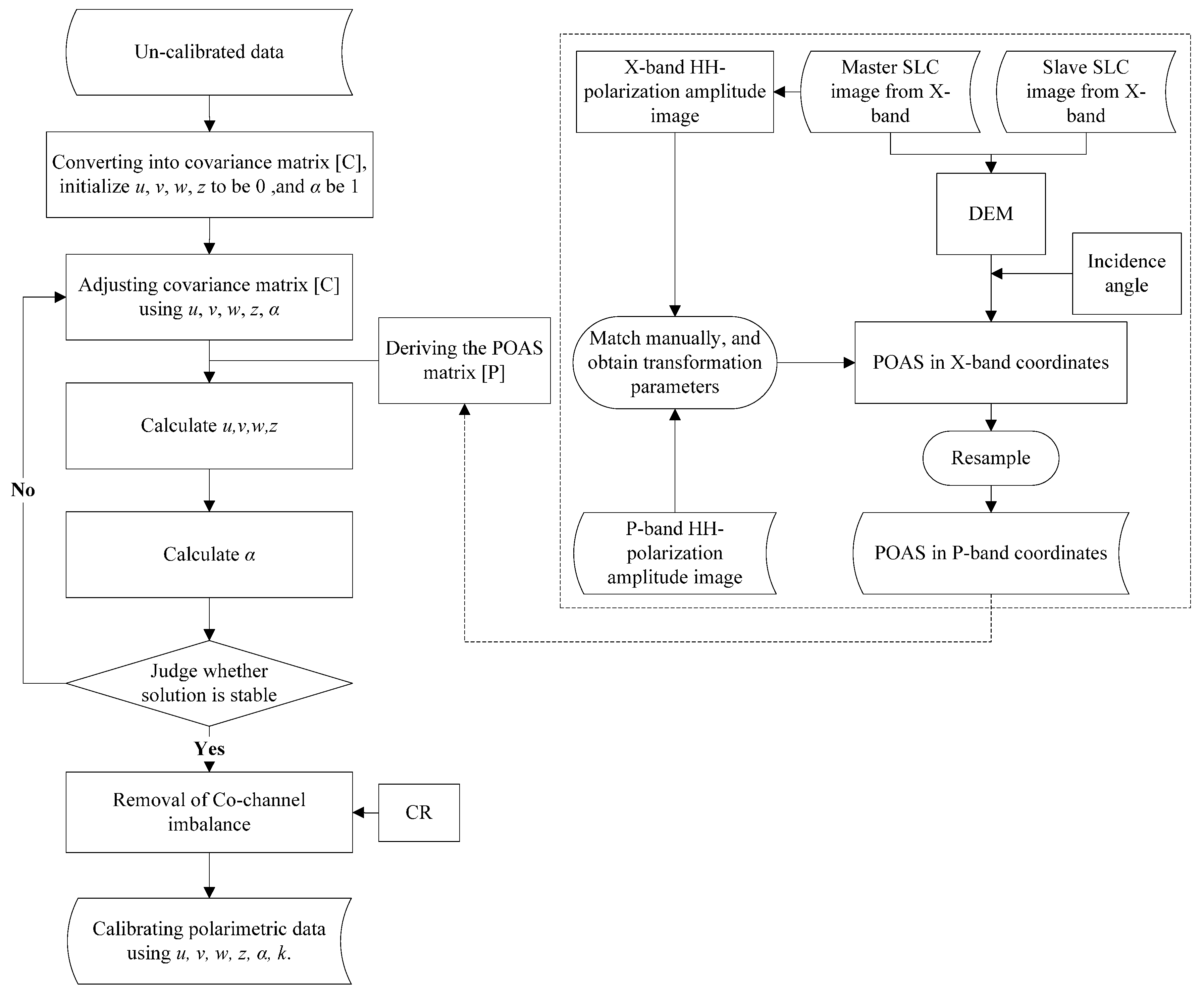
4. The Proposed PolCAL Scheme

Whether in a calibration site or not, once the un-calibrated data are acquired, the proposed technique is implemented in several steps. Firstly, the POAS of the P-band is derived through dual-band registration. Secondly, the crosstalk and cross-pol channel imbalance are calculated iteratively by assuming the reflection symmetry and reciprocity of the distributed targets. Finally, the co-pol channel imbalance is removed using the latest estimation from the CRs in the calibration site. The detailed process flow of the scheme is shown in Figure 3.

4.1. Process of Deriving the POAS

To derive an accurate POAS for P-band data, it is necessary to undertake several steps in advance. A detailed flowchart of the method is shown in the dashed box in the right part of Figure 2. The process of deriving the POAS is carried out as follows.
Step (1) A DEM is generated from the X-band data using single-pass dual-antenna interferometry.
Step (2) The POAS is calculated by Equation (7). The azimuth slope and the range slope are derived from the DEM. The incidence angle can be acquired from the metadata.
Step (3) The P-band HH-polarization amplitude image is used as the reference image for the image registration. Correspondingly, the X-band single HH-polarization amplitude image from the master SLC interferometric synthetic aperture radar (InSAR) data is treated as the target image. The two sets of corresponding control points are manually selected and matched. The transformation parameters between the two images are estimated using a two-order polynomial model.
Step (4) Because the DEM and X-band master image have the same coordinates, the POAS data are transformed and re-sampled using the calculated registration parameters between the P-band image and the X-band image.
Figure 3. Process flow of the proposed polarimetric calibration (PolCAL) technique. POAS, polarization orientation angle shift (POAS); CR, corner reflector.
Remotesensing 07 04784 g003

4.2. Solving the Crosstalk and Cross-Pol Channel Imbalance

To reduce the complexity of the solution, without introducing any serious errors, Equation (11) is simplified to 80 items by dropping all of the second-order and higher terms. After linearization with respect to u, v, w and z, the four parameters can be estimated from solving the linear equations (DHVHH = 0, DVHHH = 0, DHVVV = 0, DVHVV = 0). Using the crosstalk parameters that are estimated, DHVHV and DVHVH are obtained, and the cross-pol channel imbalance can be subsequently determined by DHVHV and DVHVH. It should be noted that DHVHV and DVHVH are calculated by the use of the estimated crosstalk parameters, without ignoring the second-order and higher terms.
In order to improve the numerical stability, the crosstalk and cross-pol channel imbalance are corrected iteratively. The calculation process is terminated when the crosstalk and channel imbalance converge. We set ||crosstalknewcrosstalkold|| ≤ 1010 or 100 iterations as the convergence conditions.

5. Experiments

The CASMSAR system has undertaken more than 200 flights in China since 2009 and has carried out a series of missions. The missions have included system calibration, topographic mapping in the Qinling Mountain Area and in the Hengduan Mountain Area and the Yushu earthquake disaster emergency response. In this study, a calibration experiment for a mountainous site with CRs was executed to validate the proposed technique. The effectiveness of the proposed technique was tested using CASMSAR data with an array of trihedral CRs. We treated the distortion parameters obtained by the trihedral CRs as the ground validation. We then used the proposed technique to estimate these parameters and compared them with the ground validation and the results of the Quegan method [4] and the Ainsworth method [29]. The CASMSAR test data were acquired in Xichang, Sichuan Province, China, in the Hengduan Mountain Area, on 25 October 2010.

5.1. Result and Evaluation of Deriving the POAS

There are two HH-polarization amplitude images shown in Figure 4a. As the reference image, the P-band image is shown in the right part of Figure 4a. The X-band image is treated as the target image and is shown in the left part of Figure 4a. In Figure 4a, seven trihedral CRs are deployed in the middle of the image along the range. We selected these trihedral CRs as a part of the ground control points (GCPs) for matching, and they are numbered as GCP 1 to 7. In addition, we also manually selected the other three feature points as GCP 8 to 10. After the 10 pairs were manually selected, the transformation model and the registration errors were computed to evaluate the registration accuracy. The registration errors consist of the error in the x- and y-directions, the root-mean-square error (RMSE) and the total RMSE. These errors are listed in Table 2. Table 2 shows that this registration process has a good accuracy and can be used to derive the POAS. As a result of using the same transformation model, the DEM from the X-band interferometry is used for the registration of the P-band image and to generate the POAS for the P-band. Finally, the results are shown in Figure 4b,c.
Figure 4. (a) Manual matching, with the left amplitude image acquired in the X-band HH-polarization, and the right amplitude acquired in the P-band HH-polarization; (b) Overlapped image of the X-band single-pass interferometric DEM image and the P-band HH amplitude image; (c) The POAS derived from the X-band interferometric DEM. The near range is at the top of image.
Remotesensing 07 04784 g004
Table 2. Evaluation measurements of the GCPs from Figure 3a in pixels.
GCPs#1#2#3#4#5#6#7#8#9#10
Error in x0.0033−0.02030.0316−0.0159−0.0033−0.00470.00280.0000−0.0001−0.0000
Error in y0.0041−0.02550.0397−0.0200−0.0041−0.00590.00350.0000−0.0001−0.0000
RMSE0.00520.03250.05070.02550.00530.00760.00450.00000.00010.0000
Total RMSE: 0.021011 pixels; Unit: Pixel.

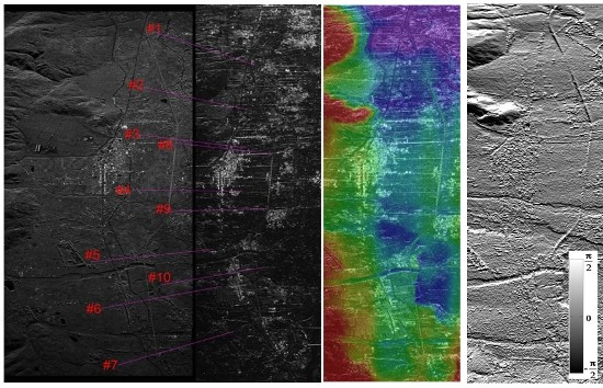
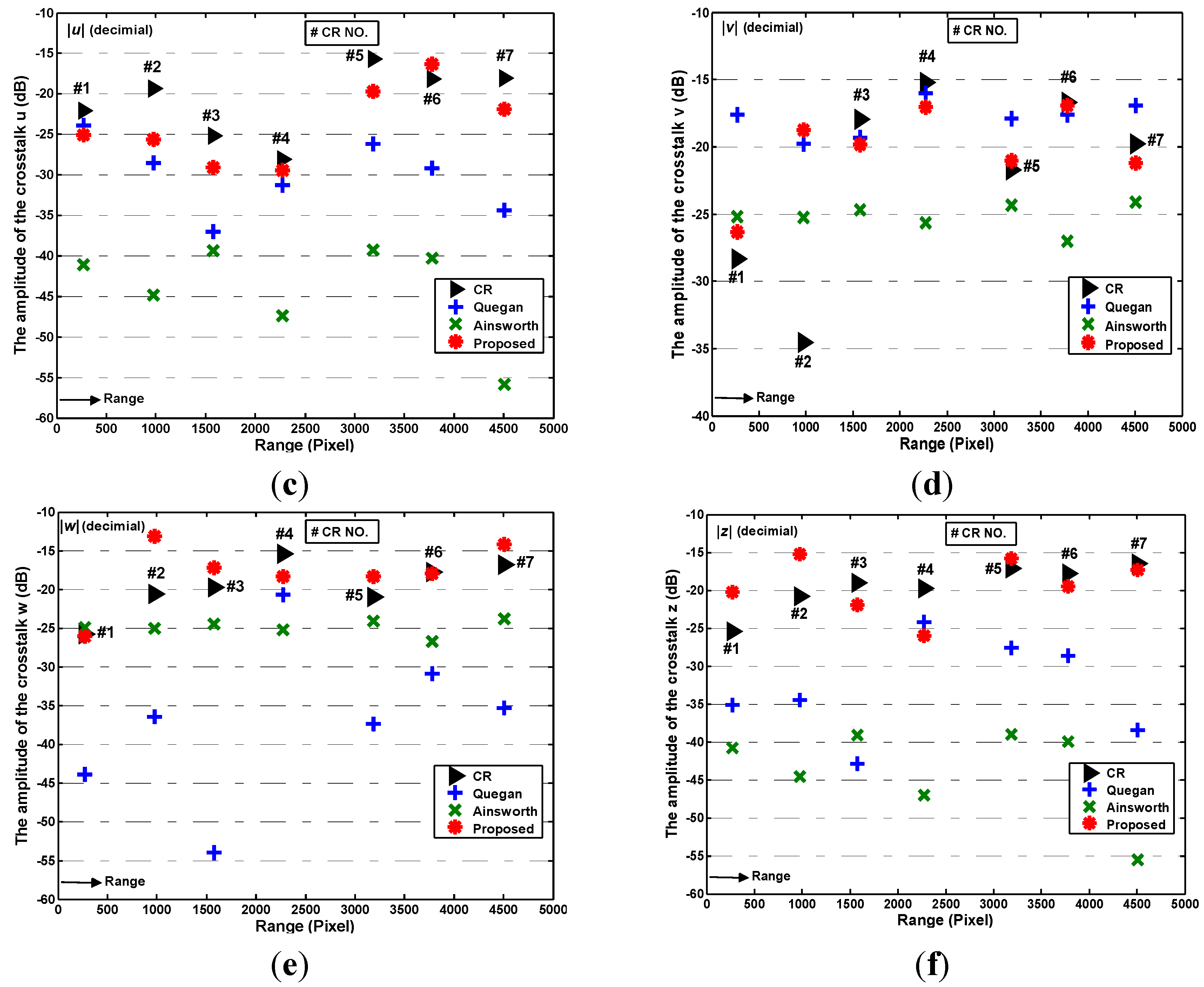
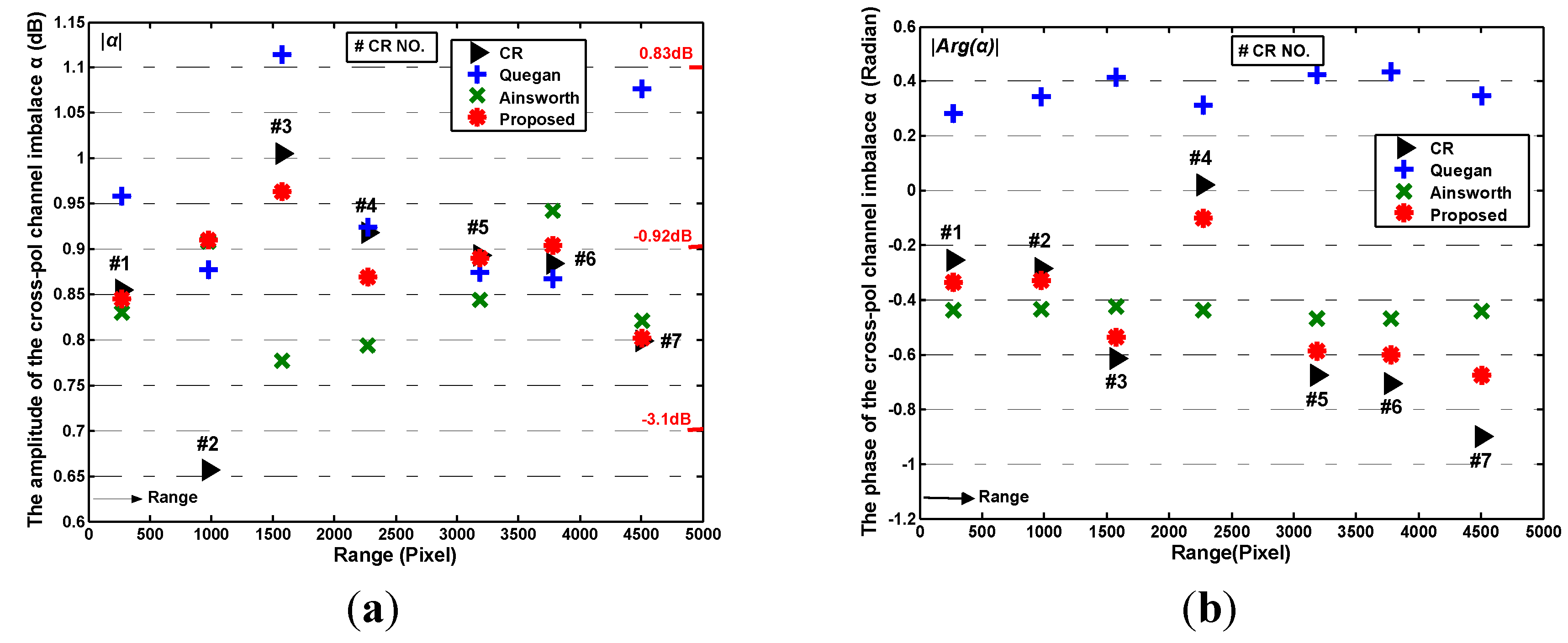
5.2. Result and Evaluation of the Crosstalk and Cross-Pol Channel Imbalance Estimation

Figure 5 shows that the results of the proposed method present a better performance than the Quegan method [4] and the Ainsworth method [29]. Using the proposed method, the estimated value of all of the points is close to the ground validation, except for CR 2. For both the crosstalk and the cross-pol channel imbalance, the worst result appears in CR 2. On the other hand, using the CR method, the estimated amplitude of the cross-pol channel imbalance in CR 2 is far from the other six points. In the RGB images of Table 3, we can see that the surroundings of CR 2 are complicated and the focus is unclear. Additionally, the biggest POAS is displayed in CR 2 due to being affected by a severe slope from Table 3. We assume that CR 2 was wrongly deployed, so that CR 2 is excluded from the ground validation. After excluding CR 2, the difference between the estimated average amplitude value of the crosstalk and the ground validation is only 1.6 dB. In addition, the amplitude difference of the cross-pol channel imbalance is 0.018, and the phase difference is 0.089 in radians. In Figure 5, the highest accuracy of the Quegan method is displayed in CR 4. The main reason for this is that this CR is deployed in a flat area, and most pixels of this azimuth are little affected by the terrain. In Table 3, the smallest slope and POAS are located in CR 2. However, the total accuracy of the Quegan method is low. In addition to the terrain effect, the observed value averaging and the calibration target selection may also have impacted the accuracy, but these issues are not the main focus of this paper. We can see that the Ainsworth method obtains very poor results. The major reason for this is that the order of the solution is the reverse of the direction of the real distortion. Moreover, using the Ainsworth method, the estimated u is approximately equal to z. Likewise, v is approximately equal to w. These weaknesses are shown in Figure 5c–f.
Figure 5. Comparison of the four methods. (ab) The amplitude and phase of α; (cf) The amplitude of u, v, w, and z.
Remotesensing 07 04784 g005aRemotesensing 07 04784 g005b
Table 3. Position information of the CRs (GCPs #1–7) in Figure 4a.
CR ##1#2#3#4#5#6#7
Pauli RGB Remotesensing 07 04784 i001 Remotesensing 07 04784 i002 Remotesensing 07 04784 i003 Remotesensing 07 04784 i004 Remotesensing 07 04784 i005 Remotesensing 07 04784 i006 Remotesensing 07 04784 i007
Land coverBare soilBare soil/CroplandBare soil/CroplandBare soil/CroplandGrass/Bare soil/Cropland/Bare soilBare soil/Buildings
Slope in range0.77974.87561.01643.0743−18.8959−4.2253−22.3820
Slope in azimuth−16.3805−24.8712−13.7515−1.5374−10.0782−6.794216.3032
Incidence26.687330.045332.933836.263140.646243.477246.9358
POAS−33.9289−47.3621−24.8353−2.7980−11.0384−9.125916.1233
Unit: Degree.

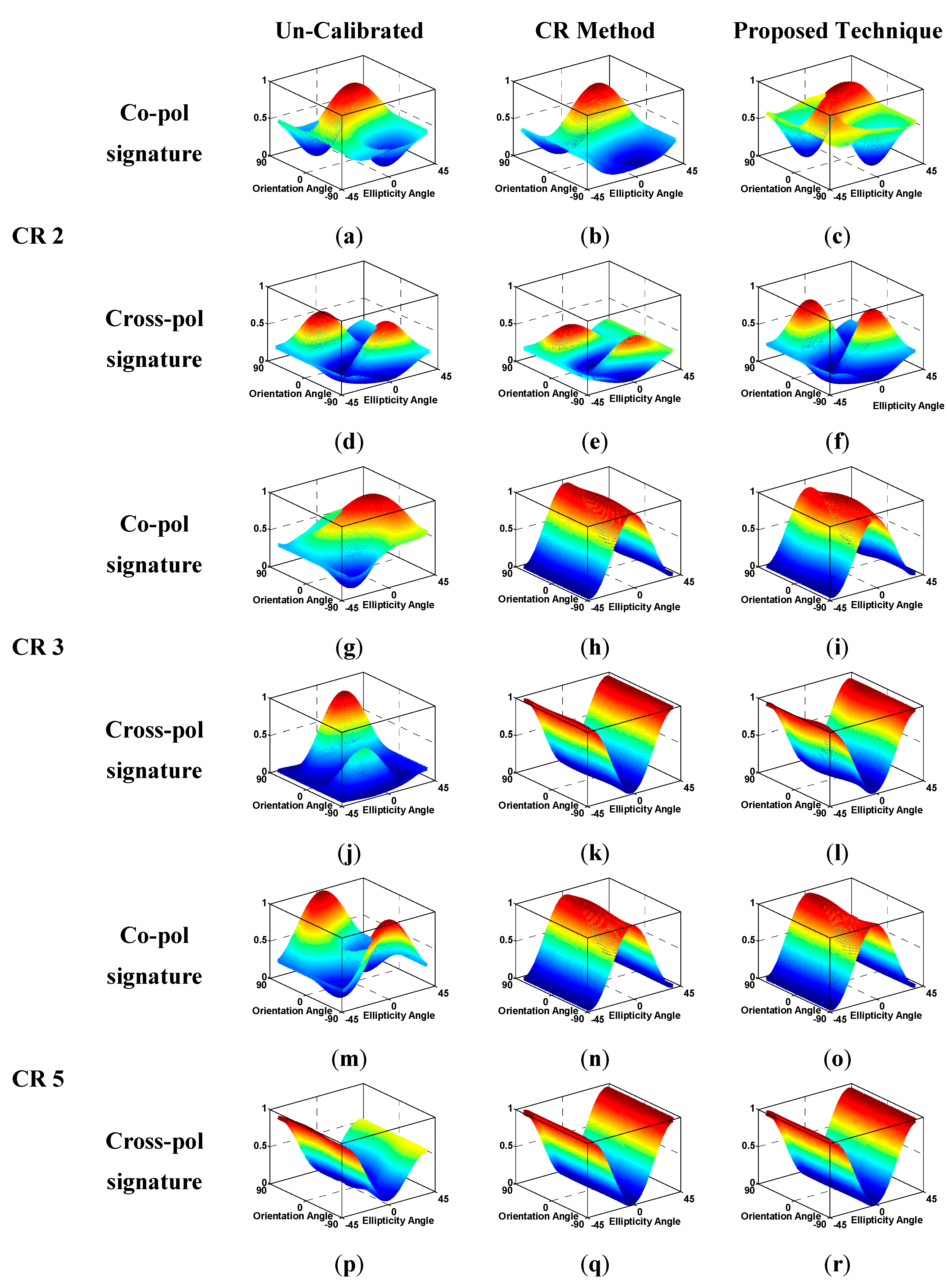
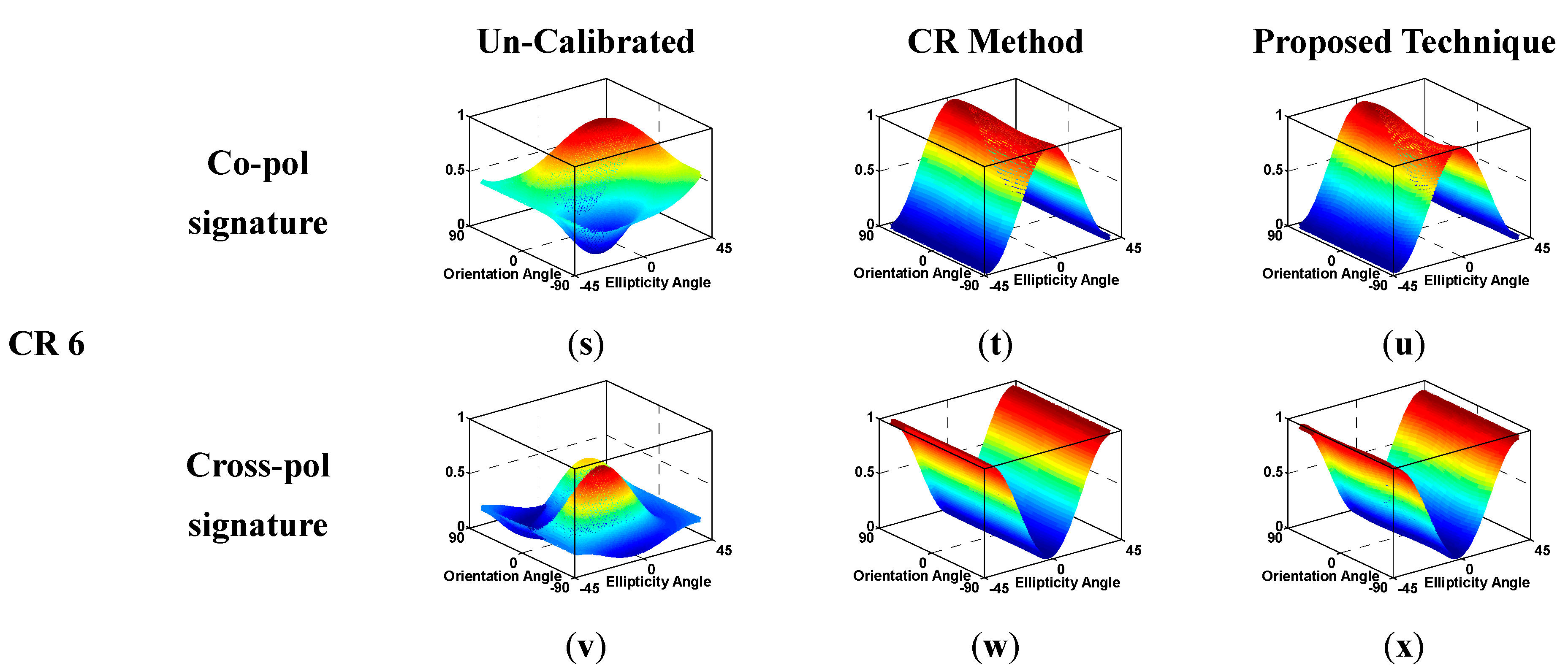
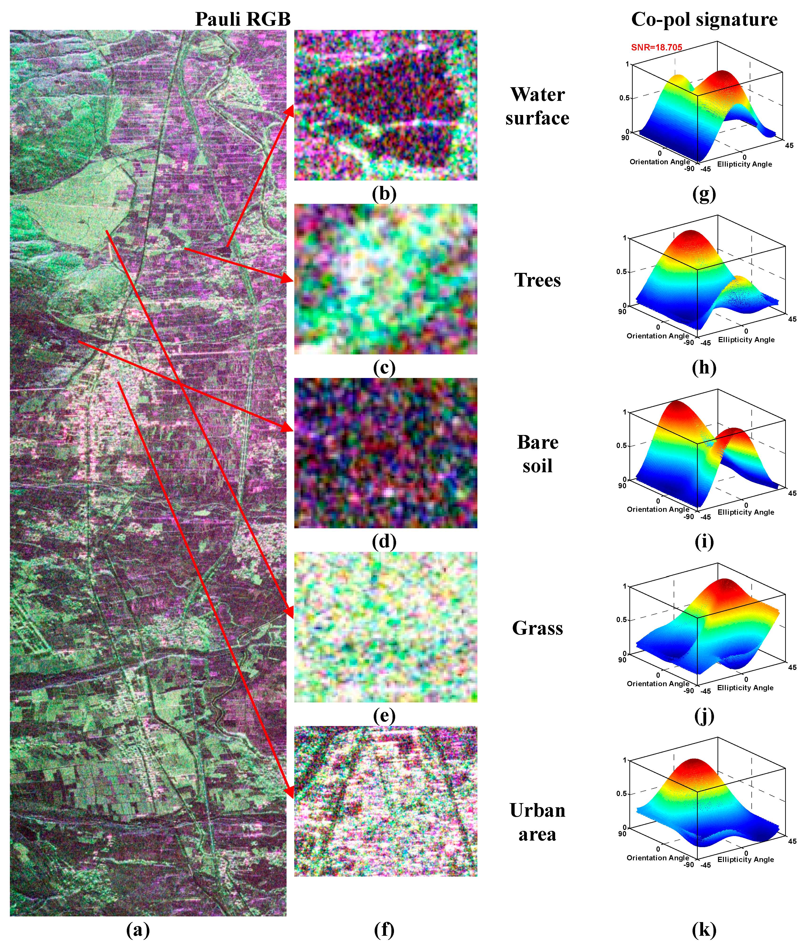
5.3. Polarimetric Signature Response

To evaluate the calibration results, the polarimetric signatures are visually displayed in Figure 6 and Figure 7. Firstly, the polarimetric signatures from several CRs are used to show the difference between the proposed technique and the CR method. Finally, combining the RGB image through Pauli decomposition and polarimetric signatures from several typical distributed targets, we could evaluate the results of the proposed technique in an upper bound of the noise floor.
Figure 6. Polarimetric signatures of the four CRs in several cases. (ac) The Co-pol signature of CR 2; (df) The Cross-pol signature of CR 2; (gi) The Co-pol signature of CR 3; (jl) The Cross-pol signature of CR 3; (mo) The Co-pol signature of CR 5; (pr) The Cross-pol signature of CR 5; (su) The Co-pol signature of CR 6; (vx) The Cross-pol signature of CR 6. From left to right, the signatures represent the results of un-calibrated, CR method and the proposed technique, respectively.
Remotesensing 07 04784 g006aRemotesensing 07 04784 g006b
We selected four different CRs (CR 2, 3, 5, 6) as representative samples. In the preceding discussion, the deployment of CR 2 was questioned, so we selected it as a sample in this section. From Figure 5, CR 3 provides the worst results in all of the parameters for the crosstalk and cross-pol channel imbalance. CR 5 presents the best cross-pol channel imbalance and the worst crosstalk. CR 6 presents the best crosstalk and a good cross-pol channel imbalance. Column 1 of Figure 6 shows the original un-calibrated polarimetric signature of the four trihedral CRs. It is clear that all of the signatures show noticeable distortions in Column 1. Column 2 of Figure 6 shows the measured polarimetric signatures of the four CRs after the CR method calibration. In Figure 6a–f, the polarimetric signatures again show that the deployment of CR 2 has serious problems, and CR 2 should be excluded from the ground validation. However, all of the other points are perfectly corrected and are close to the ideal polarimetric signature. We can see that the CR method has the best performance, and its results are close to the ground validation. When the signatures in Column 3 of Figure 6 are compared with the corresponding original un-calibrated signatures of the trihedral CRs, we can see that these signatures show a significant improvement, and they are closer to the ideal polarimetric signatures, but are not as good as the results from the CR method calibration. Comparing these to the polarization signatures after CR method calibration, it is clear that both results are in good agreement. From Figure 5, we can see that the signature of CR 3 shows the worst result in Figure 6, on account of the bad parameters. The error in CR 3 represents the largest residual error of the proposed calibration technique. Even though the largest difference between the estimated crosstalk value and the ground validation in CR 5 is 4 dB, the polarimetric signatures still show good accuracy. The reason for this is that the cross-pol channel imbalance is accurately estimated and plays a dominant role in the distortion. In Figure 6s–z, the best crosstalk result is estimated in CR 6, but the polarimetric signatures show worse results than in CR 5. This phenomenon occurs due to the estimated cross-pol channel imbalance in CR 6 being worse than in CR 6.
Figure 7. (af) RGB images by Pauli decomposition. (gk) Col-pol signatures of the five typical distributed targets.
Remotesensing 07 04784 g007
Five different land cover types (water surface, trees, bare soil, grass, urban area) are selected as typical distributed targets from the RGB image through Pauli decomposition after calibration in Column 1 and Column 2 of Figure 7. To avoid terrain effects, these objects are located in a flat area. According to [35], we can get a rough estimate of noise power from a Bragg scatterer, such as a water surface or a dry lake bed. Due to weak return and the nonzero signal in the HV measurements from actual targets, this estimate is not equal to noise, but is regarded as an upper bound to the noise floor. Using water surface in Figure 7b, the estimated signal-to-noise ratio (SNR) is 18.705 dB and considered as a high level. Column 3 of Figure 7 shows the co-pol signature of the five typical targets due to the available pedestal. The higher SNR means the lower pedestal height of the col-pol response from the Bragg scatterer. In Figure 7g, the nearly zero pedestal height of the col-pol signature shows that this proposed technique does not introduce low SNR, and this SNR should be acceptable. If there is a high SNR, the pedestal implies the randomness of scatterers. In Figure 7h–k, the col-pol signatures of the other targets have different pedestal heights that are consistent with the randomness of these targets. This proposed technique does not damage the relationship between pedestal height and randomness.

6. Discussion

In the above sections, we presented a PolCAL technique for airborne polarimetric P-band SAR data in rugged areas that makes use of concurrent X-band interferometric data (DEM). The deployed corner reflectors were used to validate the proposed method and to compare with other methods. In this section, we discuss the technique in several following points: different penetration capability influence, the co-pol channel imbalance estimation and the portability of the technique.
For the different penetration capabilities from X-band and P-band, we need to solve two problems: how to complete registration and how to extract the POAS in vegetated areas. In order to complete registration between X-band and P-band images, we could select only the artificial targets, such as buildings and roads [36]. From Figure 8b,c, CR 5 is not affected by the different bands, and the roads are displayed by similar bright lines. In the areas without artificial targets, the registration would become more difficult. In Figure 8, the main difference of the two-band HH-polarization images are displayed in an area with trees due to the different penetration capability. However, we only need to select one image as the calibration site, rather than all images for calibration. Additionally, the only image should be selected based on more feature points in this image. According to the above, we could usually avoid the differences between X-band and P-band in vegetated areas and complete registration. However, for the POAS extraction in vegetated areas, the proposed method would not acquire accurate asymmetry information using different bands. Because of the disadvantage, our future work will focus on the development of the PolCAL technique to obtain and process asymmetry information in vegetated areas.
Figure 8. (a) Optical image from Google Earth. (b) X-band HH-polarization amplitude image. (c) P-band HH-polarization amplitude image. CR 5 is displayed inside the red circle; bright points indicate the CR.
Remotesensing 07 04784 g008
Most methods relying on distributed targets solved only the crosstalk and x-pol channel imbalance, such as the Quegan method [4] and the Ainsworth method [29]. For the co-pol channel imbalance estimation, several methods without CR have been proposed [6,32]. However, these methods usually obtained worse accuracy than using the CR method and were limited in some special distributed targets. Due to the inaccuracy and limitation, we do not recommend these methods and take advantage of the latest result of the co-pol channel imbalance estimation from the CRs. In other words, the crosstalk and the x-pol channel imbalance would also be updated automatically without CRs, but the old co-pol channel imbalance would be kept until the available CRs return. Besides, the calibration parameters are usually varied from near range to far range. To control the entire image, the crosstalk and x-pol channel imbalance are estimated by the distributed targets from near range to far range. However, the co-pol channel imbalance is estimated by the CR. More accurate estimation needs more CRs. A single dihedral corner meets the minimum requirements.
The portability of the proposed technique focuses on how other source DEM should be conducted so as to extract the POAS of the corresponding polarimetric data. POAS is mainly induced by the azimuth slope and is also a function of the range slope and the radar look angle. Using the other DEM, the azimuth slope and the range slope could be firstly estimated when the radar sight direction and flight direction are known. Then, the radar look angle needs to be changed and kept consistent with the observed polarimetric data. By following the mentioned steps, the other DEM could be used to estimate the POAS of the corresponding polarimetric data. However, the different resolution might introduce some errors, especially in the fusion of low-resolution DEM and high-resolution polarimetric image [37]. In addition, the shadow effect should be considered among data acquired in rugged areas. Multi-direction acquisitions and multi-source data fusion might be able to eliminate the shadow effect and acquire complete coverage of DEM in rugged and mountainous areas.

7. Conclusions

In this paper, we have proposed a new technique to provide PolCAL and monitoring for the CASMSAR system in mountainous areas, without the use of CRs. The other multi-band airborne SAR systems with fully-polarimetric interferometry, which are similar to the CASMSAR system, could also apply this technique. The DEM generated from interferometry in the X-band can provide a priori asymmetry information (the POAS) for the fully-polarimetric P-band data. The synchronicity and the manual registration is capable of ensuring a high accuracy in the dual-band fusion. Using the POAS, the calibration model relying on distributed targets is determined and segmented into two parts for solving. The crosstalk and cross-pol channel imbalance are iteratively determined, and the proposed method was found to be closer to the results from using CRs than the results of the Quegan [4] and Ainsworth [29] methods. The displayed polarimetric signatures from several CRs show that the proposed technique could be similar to using the CR method. Additionally, this proposed technique maintained high SNR and did not damage the randomness of several typical distributed targets. Our future work will focus on the development of the PolCAL technique to obtain and process asymmetry information in vegetated areas.

Acknowledgments

The authors would like to acknowledge the support of the National Natural Science Foundation of China (Grants 61371199 and 91338111), the National High-Technology Research and Development Program (Grant 2011AA120404) and the Fundamental Research Funds for the Central Universities (Grant 2042014kf0079). The authors would also like to thank Xiangguo Lin of the Chinese Academy of Surveying and Mapping for his careful reading and all of the anonymous reviewers for their very valuable comments.

Author Contributions

Pingxiang Li and Jie Yang conceived of the research theme and undertook the research. Lu Liao designed the experiments, analyzed the results and wrote the manuscript. Fenfen Hua was responsible for the DEM generation. Jie Yang modified the manuscript. All of the authors have seen and approved the final manuscript.

Conflicts of Interest

The authors declare no conflict of interest.

References

  1. Freeman, A. SAR calibration: An overview. IEEE Trans. Geosci. Remote Sens. 1992, 30, 1107–1121. [Google Scholar] [CrossRef]
  2. Freeman, A.; van Zyl, J.J.; Klein, J.D.; Zebker, H.A.; Shen, Y. Calibration of stokes and scattering matrix format polarimetric SAR data. IEEE Trans. Geosci. Remote Sens. 1992, 30, 531–539. [Google Scholar] [CrossRef]
  3. Quegan, S. A unified algorithm for phase and cross-talk calibration of polarimetric data-theory and observations. IEEE Trans. Geosci. Remote Sens. 1994, 32, 89–99. [Google Scholar] [CrossRef]
  4. Klein, J.D. Calibration of complex polarimetric SAR imagery using backscatter correlations. IEEE Trans. Aerosp. Electron. Syst. 1992, 28, 183–194. [Google Scholar] [CrossRef]
  5. Sarabandi, K. Calibration of a polarimetric synthetic aperture radar using a known distributed target. IEEE Trans. Geosci. Remote Sens. 1994, 32, 575–582. [Google Scholar] [CrossRef]
  6. Shimada, M. Model-based polarimetric SAR calibration method using forest and surface-scattering targets. IEEE Trans. Geosci. Remote Sens. 2011, 49, 1712–1733. [Google Scholar] [CrossRef]
  7. Shimada, M.; Freeman, A. A technique for measurement of spaceborne SAR antenna patterns using distributed targets. IEEE Trans. Geosci. Remote Sens. 1995, 33, 100–114. [Google Scholar] [CrossRef]
  8. Zink, M.; Rosich, B. Antenna elevation pattern estimation from rain forest acquisitions. In Proceedings of CEOS Working Group on Calibration/Validation—SAR Workshop, London, UK, 24–26 September 2002.
  9. Attema, E.; Brooker, G.; Buck, C.; Desnos, Y.-L.; Emiliani, L.; Geldsthorpe, B.; Laur, H.; Laycock, J.; Sanchez, J. ERS-1 and ERS-2 antenna pattern estimates using the Amazon Rain Forest. In Proceedings of CEOS SAR Workshop RADARSAT Data Quality, Saint-Hubert, QC, Canada, 4–6 February 1997.
  10. Van Zyl, J.J. Calibration of polarimetric radar images using only image parameters and trihedral corner reflector responses. IEEE Trans. Geosci. Remote Sens. 1990, 28, 337–348. [Google Scholar] [CrossRef]
  11. Sarabandi, K.; Pierce, L.E.; Ulaby, F.T. Calibration of a polarimetric imaging SAR. IEEE Trans. Geosci. Remote Sens. 1992, 30, 540–549. [Google Scholar] [CrossRef]
  12. Christensen, E.L.; Skou, N.; Dall, J.; Woelders, K.W.; Jorgensen, J.H.; Granholm, J.; Madsen, S.N. EMISAR: An absolutely calibrated polarimetric l- and c-band SAR. IEEE Trans. Geosci. Remote Sens. 1998, 36, 1852–1865. [Google Scholar] [CrossRef]
  13. Horn, R.; Scheiber, R.; Buckreuss, S.; Zink, M.; Moreira, A.; Sansosti, E.; Lanari, R. E-SAR generates level-3 SAR Products for ProSmart. In Procedings of the Geoscience and Remote Sensing Symposium, IEEE 1999 International, Hamburg, Germany, 28 June–2 July 1999.
  14. Satake, M.; Kobayashi, T.; Uemoto, J.; Umehara, T.; Kojima, S.; Matsuoka, T.; Nadai, A.; Uratsuka, S. Polarimetric calibration of PI-SAR2. In Proceedings of the 2013 Asia-Pacific Conference on Synthetic Aperture Radar (APSAR), Tsukuba, Japan, 23–27 September 2013.
  15. Touzi, R.; Shimada, M. Polarimetric PALSAR calibration. IEEE Trans. Geosci. Remote Sens. 2009, 47, 3951–3959. [Google Scholar] [CrossRef]
  16. Matsuoka, T.; Umehara, T.; Nadai, A.; Kobayashi, T.; Satake, M.; Uratsuka, S. Calibration of the high performance airborne SAR system (PI-SAR2). In Proceedings of the 2009 IEEE International Geoscience and Remote Sensing Symposium (IGARSS 2009), Cape Town, South Africa, 12–17 July 2009.
  17. Satake, M.; Matsuoka, T.; Umehara, T.; Kobayashi, T.; Nadai, A.; Uemoto, J.; Kojima, S.; Uratsuka, S. Calibration experiments of advanced x-band airborne SAR system, PI-SAR2. In Proceedings of the 2011 IEEE International Geoscience and Remote Sensing Symposium (IGARSS), Seoul, Korea, 24–29 July 2011.
  18. D’Aria, D.; Ferretti, A.; Monti Guarnieri, A.; Tebaldini, S. SAR calibration aided by permanent scatterers. IEEE Trans. Geosci. Remote Sens. 2010, 48, 2076–2086. [Google Scholar] [CrossRef]
  19. Iannini, L.; Tebaldini, S.; Guarnieri, A.M. Long term relative polarimetric calibration by natural targets. In Proceedings of the 2013 IEEE International Geoscience and Remote Sensing Symposium (IGARSS), Melbourne, Australia, 21–26 July 2013.
  20. Zhang, J.; Zhao, Z.; Huang, G.; Lu, Z. CASMSAR: An integrated airborne SAR mapping system. Photogramm. Eng. Remote Sens. 2012, 78, 1110–1114. [Google Scholar]
  21. Zhang, J.; Wang, Z.; Huang, G.; Zhao, Z.; Lu, L. CASMSAR: The first Chinese airborne SAR mapping system. In Proceedings of the Earth Observing Systems XV, San Diego, CA, USA, 3–5 August 2010.
  22. Zhang, J.; Cheng, C.; Huang, G. Block adjustment of POS-supported airborne SAR images. In Proceedings of the International Radar Symposium, IRS 2011, Leipzig, Germany, 7–9 September 2011.
  23. Huang, G.; Yang, S.; Wang, N.; Zhang, J.; Zhao, Z. Block combined geocoding of airborne InSAR with sparse GCPs. Acta Geod. Cartogr. Sin. 2013, 42, 397–403. [Google Scholar]
  24. Zhao, Z.; Zhang, J.; Huang, G.; Hua, F.; Yang, S.; Deng, S. High-resolution airborne SAR interferometry mapping application in Huashan Mountain. In Proceedings of the 2010 Second IITA International Conference on Geoscience and Remote Sensing (IITA-GRS), Qingdao, China, 28–31 August 2010.
  25. Yang, S.; Huang, G.; Zhao, Z. A method for generation of SAR stereo model with image simulation. Geomat. Inf. Sci. Wuhan Univ. 2012, 37, 1325–1328. [Google Scholar]
  26. Lee, J.S.; Schuler, D.L.; Ainsworth, T.L.; Krogager, E.; Kasilingam, D.; Boerner, W.M. On the estimation of radar polarization orientation shifts induced by terrain slopes. IEEE Trans. Geosci. Remote Sens. 2002, 40, 30–41. [Google Scholar] [CrossRef]
  27. Gail, W.B. Effect of Faraday rotation on polarimetric SAR. IEEE Trans. Aerosp. Electron. Syst. 1998, 34, 301–307. [Google Scholar] [CrossRef]
  28. Wright, P.A.; Shuan, Q.; Wheadon, N.S.; Hall, C.D. Faraday rotation effects on l-band spaceborne SAR data. IEEE Trans. Geosci. Remote Sens. 2003, 41, 2735–2744. [Google Scholar] [CrossRef]
  29. Ainsworth, T.L.; Ferro-Famil, L.; Lee, J.S. Orientation angle preserving a posteriori polarimetric SAR calibration. IEEE Trans. Geosci. Remote Sens. 2006, 44, 994–1003. [Google Scholar] [CrossRef]
  30. Kimura, H. Calibration of polarimetric PALSAR imagery affected by Faraday rotation using polarization orientation. IEEE Trans. Geosci. Remote Sens. 2009, 47, 3943–3950. [Google Scholar] [CrossRef]
  31. Lee, J.S.; Schuler, D.L.; Ainsworth, T.L. Polarimetric SAR data compensation for terrain azimuth slope variation. IEEE Trans. Geosci. Remote Sens. 2000, 38, 2153–2163. [Google Scholar] [CrossRef]
  32. Shi, L.; Yang, J.; Li, P. Co-polarization channel imbalance determination by the use of bare soil. ISPRS J. Photogramm. Remote Sens. 2014, 95, 53–67. [Google Scholar] [CrossRef]
  33. Zhang, H.; Lu, W.; Zhang, B.; Chen, J.; Wang, C. Improvement of polarimetric SAR calibration based on the Ainsworth algorithm for Chinese airborne POLSAR data. IEEE Geosci. Remote Sens. Lett. 2013, 10, 898–902. [Google Scholar] [CrossRef]
  34. Xing, S.-Q.; Dai, D.-H.; Liu, J.; Wang, X.-S. Comment on “orientation angle preserving a posteriori polarimetric SAR calibration”. IEEE Trans. Geosci. Remote Sens. 2012, 50, 2417–2419. [Google Scholar] [CrossRef]
  35. Freeman, A. Effects of Noise on Polarimetric SAR Data. In Proceedings of the 13th Annual International Geoscience and Remote Sensing Symposium, Tokyo, Japan, 18–21 August 1993.
  36. Zhang, J.; Lin, X. Semi-automatic extraction of straight roads from very high resolution remotely sensed imagery by a fusion method. Sens. Lett. 2013, 11, 1229–1235. [Google Scholar] [CrossRef]
  37. Zhang, J. Trends in geo-information fusion for the next 5 years. Int. J. Image Data Fusion 2014, 5. [Google Scholar] [CrossRef]

