Article

A Comparison of Novel Optical Remote Sensing-Based Technologies for Forest-Cover/Change Monitoring

Department of Plant Sciences, University of Cambridge, Downing Street, Cambridge CB2 3EA, UK
*
Author to whom correspondence should be addressed.
Remote Sens. 2015, 7(3), 2781-2807; https://doi.org/10.3390/rs70302781
Submission received: 22 December 2014 / Revised: 11 February 2015 / Accepted: 4 March 2015 / Published: 10 March 2015

Abstract

:
Remote sensing is gaining considerable traction in forest monitoring efforts, with the Carnegie Landsat Analysis System lite (CLASlite) software package and the Global Forest Change dataset (GFCD) being two of the most recently developed optical remote sensing-based tools for analysing forest cover and change. Due to the relatively nascent state of these technologies, their abilities to classify land cover and monitor forest dynamics have yet to be evaluated against more established approaches. Here, we compared maps of forest cover and change produced by the more traditional supervised classification approach with those produced by CLASlite and the GFCD, working with imagery collected over Sierra Leone, West Africa. CLASlite maps of forest change from 2001–2007 and 2007–2014 exhibited the highest overall accuracies (79.1% and 89.6%, respectively) and, importantly, the greatest capacity to discriminate natural from planted mature forest growth. CLASlite’s comparative advantage likely derived from its more robust sub-pixel classification logic and numerous user-defined parameters, which resulted in classified products with greater site relevance than those of the two other classification approaches. In light of today’s continuously growing body of analytical toolsets for remotely sensed data, our study importantly elucidates the ways in which methodological processes and limitations inherent in certain classification tools can impact the maps they are capable of producing, and demonstrates the need to understand and weigh such factors before any one tool is selected for a given application.

Graphical Abstract

1. Introduction

Remote sensing is becoming an increasingly indispensable tool in ecology and conservation biology [1,2,3,4], with growing traction particularly in forest monitoring. The opening of the U.S. Geological Survey’s Landsat archive, which harbours more than 2 million satellite images of the Earth’s surface dating back to 1972 [5], has revolutionised standards for the availability of Earth observation data and helped to facilitate the rise of forests as today’s most common large-area monitoring target [6]. Airborne light detection and ranging (LiDAR) technologies that emit laser pulses to obtain information in three dimensions, along with associated developments in LiDAR analytical techniques, have improved capacities to measure forest stand structure [7] and facilitated the production of high-resolution aboveground carbon density maps [8,9,10]. Very High Resolution (VHR) products (e.g., aerial photos, IKONOS, GeoEye, QuickBird) can feature sub-meter spatial resolutions that allow for the delineation of complex spatial heterogeneities in forest structure based on multi-scale segmentation [11] or texture-based [12,13] analytical approaches. The launch of many new Earth observation systems, greater access to their products, and the continued development of computational technologies for remotely sensed data are supporting satellite imagery-based global forest-cover analyses at ever higher spatial, temporal, and thematic resolutions, and testify to sustained progress in remote sensing-based forest monitoring today [14,15].
However, a number of challenges still impede the more widespread use of remote sensing technologies for natural resource monitoring, two of which we address here. First, end-users in natural resource monitoring fields may lack a technical understanding of remotely sensed datasets and their associated analyses, and thus rely upon remote sensing scientists to design and implement remote sensing-based projects [16,17]. The high level of expertise necessary to handle remotely sensed data and products is considered an outstanding challenge facing today’s ecologists and conservation biologists that has limited their ability to take full advantage of remote sensing technologies as real assets [18]. Secondly, globally (or even regionally) consistent maps of land-cover change remain unavailable because of a lack of consensus on appropriate analytical approaches [6]. Conservation planning, which often requires information on processes that occur over a range of scales, is a field for which broadly consistent data layer coverage is of high importance [19]. Indeed, the success of increasing numbers of international and national habitat monitoring systems today directly depends upon efficient and long-term biodiversity monitoring at the habitat and landscape levels [18,20].
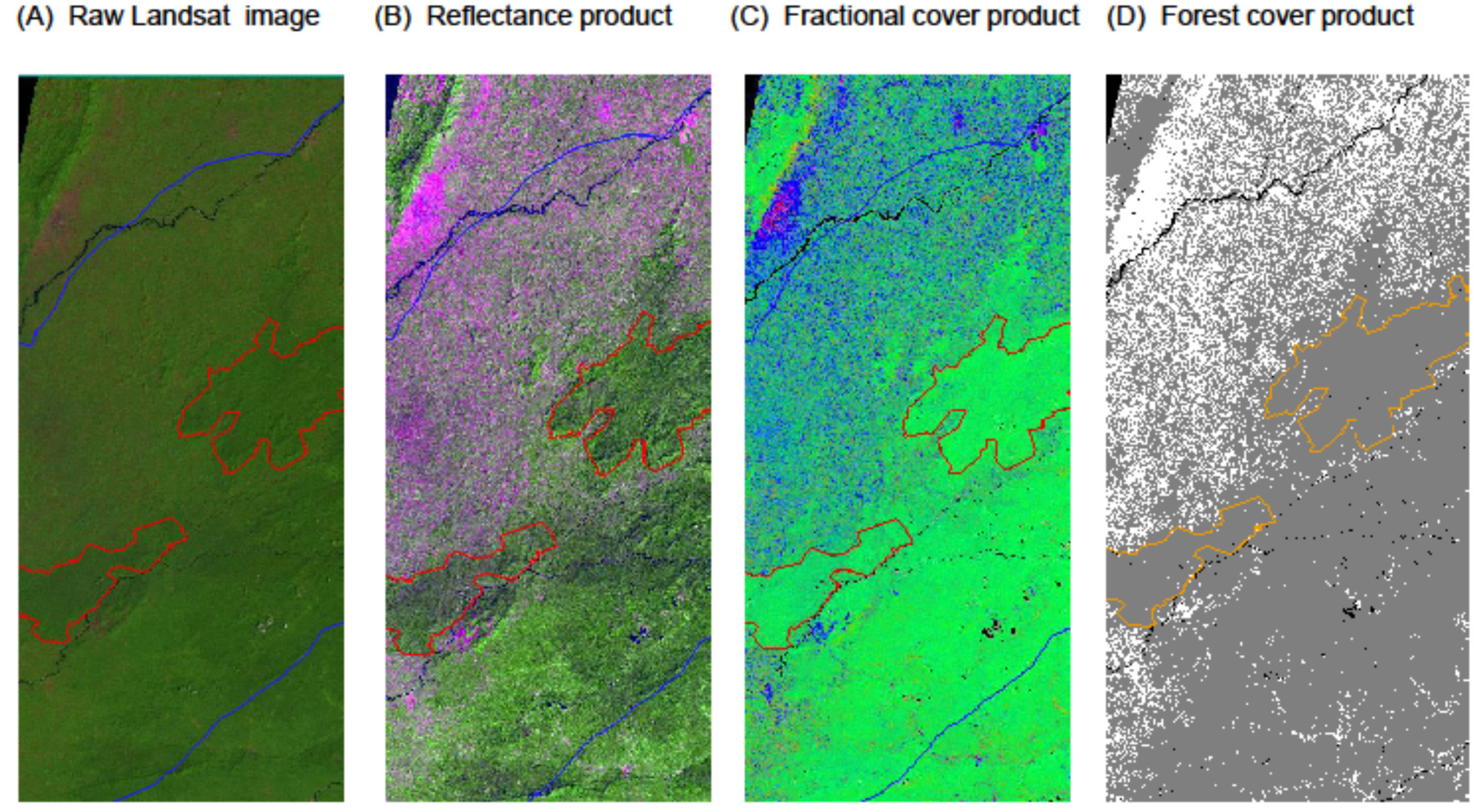
Two of the most recent technologies that have emerged in the field of remote sensing for forest monitoring address these challenges of inaccessibility to non-expert users and limited availability of globally consistent products. The Carnegie Landsat Analysis System lite (CLASlite) is a semi-automated analysis environment in which users can process radiometric data from nine different satellite systems—including the Landsat series—to produce maps of deforestation and forest disturbance. CLASlite administers the following semi-automated central functions to achieve such products: (1) Image calibration of raw satellite imagery to apparent surface reflectance; (2) fractional cover analysis of surface reflectance data into proportional estimates of photosynthetic and non-photosynthetic vegetation cover as well as bare substrate using an Automated Monte Carlo Unmixing (AutoMCU) model that draws from a representative library of reflectance spectra; (3) forest-cover classification of fractional cover data based on proportional cover of photosynthetic vegetation and bare substrate; and (4) change detection between multi-temporal fractional cover data to determine deforestation and forest disturbance over time (Figure A1). CLASlite’s AutoMCU spectral mixture analysis algorithm is reported to be capable of detecting changes in forest cover in increments as small as 1% of a Landsat pixel, which corresponds to roughly 10 m2 [21]. Thus, CLASlite offers the potential to overcome current challenges in detecting cryptic forms of tropical forest degradation such as surface fire and sub-canopy disturbances that often occur at such smaller scales [22]. The CLASlite software package became globally and freely available in December 2013; individuals may download CLASlite upon completion of an online training course [23]—the world’s first for deforestation and forest degradation mapping—that is specifically designed to empower those with limited training in remote sensing. CLASlite users have already demonstrated CLASlite’s suitability for analysing deforestation and logging in tropical regions [24,25,26].
The second product, the Global Forest Change dataset (GFCD), was made available for free public download in February 2014 and is the first medium- to high-resolution (30 m) downloadable data product detailing global forest extent, loss, and gain from 2000–2012 [27]. The GFCD is based on time-series analyses of 654,178 growing season scenes captured by the Enhanced Thematic Mapper Plus (ETM+) spectrometer on board the Landsat 7 satellite and processed in parallel using the Google Earth Engine cloud environmental analysis platform. Each Landsat scene used in the GFCD is a computationally generated mosaic of cloud-free 30 m × 30 m Landsat pixels. Considering all vegetation taller than 5 m in height as trees and defining forest loss as the removal of all trees within a pixel, the GFCD stratified pixels from Landsat growing season data into <25%, 26%–50%, 51%–75%, and 76%–100% tree-cover (in year 2000) classes and quantified the area of forest lost from 2000–2012 within each tree-cover class. Per-band metrics employed by the GFCD to characterise forest cover and change included pixel reflectance and mean reflectance values at maximum, minimum, and selected percentile values over time. Data used to train the Landsat metrics were derived from high spatial-resolution data (e.g., QuickBird imagery) and various existing percent tree cover datasets. Validation for accuracy was performed against reference change data obtained from image interpretation of time-series Landsat, Moderate Resolution Imaging Spectroradiometer (MODIS), and high spatial-resolution Google Earth™ imagery, as well as reference canopy height change LiDAR data obtained from NASA’s Geoscience Laser Altimetry System (GLAS) instrument on board the IceSat-1 satellite [27]. As a “globally consistent and locally relevant” record of forest change [27], the GFCD forms the basis of Global Forest Watch, a freely available forest monitoring and alerting database with demonstrated impacts on timely conservation action and response [28].
It is clear that both CLASlite and the GFCD harbour not only valuable utility in modern forest conservation efforts, but also the immediate potential to remove some of the barriers preventing remote sensing technologies from fully integrating with conservation communities. However, because both CLASlite and the GFCD are both relatively nascent technologies, opportunities to assess their relative capacities to classify land cover and monitor forest dynamics remain. Comparing the classification abilities of CLASlite and the GFCD is of critical importance given the array of new land-cover data, products, and tools that are available—and still being developed—today. No single technology will be optimal for all applications; rather, its suitability will depend heavily upon the requirements of the user with respect to, for example, thematic coverage, and spatial and temporal detail [29]. Because CLASlite and the GFCD differ with respect to these features as well as their inherent methodological and analytical frameworks, it is of special interest to investigate the ways in which these differences might afford either forest monitoring technology certain advantages over the other when assessing the dynamics of complex forested landscapes in ways that are meaningful to conservationists. Especially relevant to conservation studies today are technologies that can differentiate natural mature forest from mature tree growth with obvious anthropogenic origins, such as palm plantations. Technologies with the ability to make this distinction would be vital resources for zero net deforestation targets, which value both the protection of native forests and the planting of new ones, and zero gross deforestation targets, which are particularly concerned with gross loss of forest area over time and broadly aim for no deforestation anywhere [30]. Remote sensing technologies that can map tree plantations separately from native forests will also contribute to more effective monitoring and a greater understanding of the impacts of land conversion due to growth in commercial agriculture [31,32], and critically inform carbon credit schemes such as the United Nation’s Reducing Emissions from Deforestation and Forest Degradation (REDD) Programme [33,34].
To deepen our assessment of the relative utilities of CLASlite and GFCD in forest monitoring, we further compared their classification abilities with those of supervised classification, a more established and traditional pixel-based land classification technique. Supervised classification is predicated upon user knowledge of the realities of a given study site; clusters of training pixels in a satellite image that are representative of any number of user-defined land-cover categories of interest are first identified by the user, then used to train a specified classification algorithm to locate and identify similar pixels in the remainder of the image [35]. While the a priori input of information has been identified as the main disadvantage of the supervised approach due to its potentially difficult, subjective, and time-consuming nature [36], the site-specific scope of our study as well as our use of high-resolution Google Earth™ imagery to promote the accurate identification of training pixels (see Section 2.3 for more detailed methodology) mitigated these concerns. Other common classification methods such as unsupervised classification and object based image analysis (OBIA) were considered less optimal for this study when compared with the supervised approach. Unsupervised classification, in which a classification algorithm is used to automatically assign image pixels into a user-defined number of classes, still requires significant post-classification labelling and has been shown to produce suboptimal results when compared to supervised classification [37]. Meanwhile, OBIA involves segmenting an image into clusters of neighbouring pixels—or “objects”—that share similar spectral properties (i.e., digital values) as well as other semantically significant properties (e.g., size, shape, geography) [38]. However, OBIA is considered a more appropriate tool when segmenting and extracting features from VHR data, in which pixels are substantially smaller than the objects of classification interest (e.g., individual tree crowns) [39]. Not only are per-pixel based classification methods such as supervised classification considered more appropriate when using Landsat imagery [40], as was the case with our study, but supervised land classification is also considered a classic and the most widely used quantitative land-cover mapping approach [41,42]—a ubiquity which further supported our decision to employ supervised classification as a representative traditional classification approach, against which the more contemporary classification technologies of CLASlite and the GFCD could be compared.
In this study, we tested the inherent abilities of these three classification methodologies—supervised classification, CLASlite and the GFCD—to create accurate forest cover and change maps for a region of Sierra Leone in West Africa which included Gola Rainforest National Park (hereafter Gola) since 2000. We expected that the different classification approaches fundamentally employed by the three methods would result in disparate map products, and aimed to ascertain the extent to which these differences reflected a greater utility of one approach over the others when monitoring forest dynamics over Gola. To quantify relative utility among these three classification approaches, we used the metric of extent of agreement between the predicted forest cover and loss maps generated by each of the three tools, and independently identified truth regions of forest cover and loss over the Gola area. The assessed value of each land classification approach was also heavily dependent upon its ability to make the difficult yet critical distinction between mature natural forest and mature anthropogenic plantations/agricultural areas, which is a growing urgency in the conservation sciences today. Thus, another key aim of our study was to create a methodology to test the ways in which the different classification algorithms and outputs inherent in the given framework of each classification approach (e.g., the binary forest/non-forest maps of CLASlite and the GFCD versus maps of any user-defined number of classes from the supervised classification) would be able to achieve this task.

2. Experimental Section

2.1. Study Area

Land cover and change classification was conducted on satellite images of Gola and its neighbouring land, located near the south-eastern border of Sierra Leone with Liberia. Covering an area of 710 km2, Gola represents the largest remaining area of lowland moist evergreen high forest in Sierra Leone [43] and forms part of the western Upper Guinean forest ecosystem, a recognised global biodiversity hotspot [44]. Gola holds most of the region’s endemic, threatened, and near-threatened mammals and birds [45]. While Gola has been protected through conservation programs since 1989, encroachment by smallholder agriculturalists serves as the primary threat and driver of deforestation in the region due to a high proportion of the population engaging in subsistence agriculture; however, illicit gold and diamond mining activities, expansion of human settlements, sporadic farming, poaching, industrial agriculture (e.g., oil palm or coffee plantations), logging and woodcutting for domestic firewood also negatively impact the integrity of the reserve [46].
The natural vegetation type is predominantly moist evergreen lowland forest [43]. The area has a seasonal climate, with annual rainfall around 2500–3000 mm and a dry season lasting from November to April. The altitude of the park is 70–410 m. Other vegetation types within the park include moist semi-deciduous forest, freshwater inland swamp forest, secondary and disturbed forest, farmbush, herbaceous swamps, and floodplains [47]. Land cover outside of the park includes secondary and disturbed forest, farmbush and shrubland/savannah, plantation, and agriculture [48].

2.2. Landsat Satellite Imagery

To determine land cover and change in and surrounding Gola, 30 m resolution Landsat satellite images of Gola taken in 2001, 2007, and 2014 were downloaded from the United States Geological Survey Global Visualisation Viewer (GloVis) website [49]. Imagery from Landsat satellites are popular data sources for documenting changes in land cover and use over time due to their long history, reliability, and availability [15], while their 30 m resolution is considered adequate for characterising landscape patterns [50] and differentiating natural from human-induced land change [51]. The region of interest was covered by two Landsat image tiles representing Gola’s eastern and western portions, resulting in the use of six total Landsat images for this study—two from each of the three years of interest. Only images acquired in January and February were selected for use, as these months fall within the study area’s dry season when there is a greater probability of cloud-free images. Landsat imagery from 2001 and 2014 were selected, as these years were the only years closest to the respective 2000 and 2012 starting and ending years of the GFCD for which we could find adequately cloud-free imagery during January/February. Also, the year 2007 was the year closest to the midway point between 2001 and 2014 for which we could find adequately cloud-free imagery during January/February. Only images with relatively low reported cloud cover (<10%) were selected (Table A1), and all automatically received systematic, radiometric, geometric, and topographic corrections through GloVis prior to download. Satellite imagery were delivered with a projection of UTM Zone 29N using the WGS 1984 Datum.

2.3. Method 1: Supervised Land Classification

All image processing was conducted in ENVI 5.0 Classic (Exelis Visual Information Solutions, Inc., Boulder, Colorado). First, original digital number (DN) data stored for each pixel in each of the six raw Landsat image scenes of interest over Gola (Table A1) were automatically converted into top-of-atmosphere reflectance values using CLASlite v.3.1 (Carnegie Institution for Science, Stanford, California). On each of the resulting reflectance images, polygonal pixel clusters, or Regions of Interest (ROIs) belonging to six land-cover classes of interest were identified using careful visual interpretation and spectral assessments of the raw Landsat image and corroborated with high-resolution Google Earth™ imagery. The six classes were: (1) non-vegetation (e.g., bare substrate, exposed rocks, urban areas, villages), (2) mature forest (i.e., non-planted intact mature tree stands), (3) other vegetation (e.g., all other vegetative cover such as grassland and swampland, as well as tree stands with obvious anthropogenic influences such as palm plantations and agricultural land), (4) water, (5) clouds, and (6) cloud shadow. More specifically, the mature forest category comprised groups of trees identifiable through Google Earth™ imagery featuring spectral signatures characteristic of healthy and mature vegetation (as outlined in [24]). Any groups of trees whose anthropogenic influences were immediately apparent, such as recognisable monocultures or linear/otherwise unnaturally shaped plantations, were deliberately excluded from the mature forest category, and the other vegetation category was trained to include such tree stands instead. Image-edge pixels representing the boundaries of Landsat images were identified as a seventh land-cover category for ease of subsequent image processing.
More than 10,000 pixels were selected for each of ROI classes 1-3 in order to encapsulate the spectral variation within these land-cover types. Roughly 1500 pixels were identified for each of classes 4–6. All ROIs were distributed as evenly as possible over each of the six Landsat scenes. The spectral properties of the ROIs were then used to train ENVI’s Maximum Likelihood algorithm, an effective and commonly used classifier [52,53], to classify the remaining area of each scene. This algorithm assumes a normal distribution of reflectance values for each user-defined class within each spectral band of the original satellite image, and assigns each pixel to a specific class based on the probability of it belonging to that class. Due to geographic overlap between the eastern and western Landsat scenes, each of the three resulting classified maps of eastern Gola (which encompassed a greater extent of the study region) was mosaicked atop the classified map of western Gola from the same year, and clipped to a 25 km boundary around Gola. Final products from this process were three classified land-cover maps over Gola and its surrounding 25 km region from 2001, 2007, and 2014.
Forest-cover change from 2001–2007 and 2007–2014 was determined by identifying differences between the 2001, 2007, and 2014 classified maps using thematic change analysis in ENVI. Default ENVI refinement parameters setting smoothing kernel size to 3 (i.e., 3 × 3 pixels) and aggregate minimum size to 9 pixels were employed to remove “salt-and-pepper” effects. Pixels in the land-cover change maps of 2001–2007 and 2007–2014 were classified as deforested if they changed from a state of mature forest into either of the other vegetation or non-vegetation categories. Deforestation pixels were then aggregated within Gola’s boundary and within the 25 km buffer surrounding Gola, exclusive of Gola itself.

2.4. Method 2: Land Classification in CLASlite

All six raw Landsat scenes of the eastern and western portions of Gola from 2001, 2007, and 2014 (Table A1) were classified individually into forest cover using CLASlite. Default parameters for the first three of CLASlite’s four built-in steps were altered for some Landsat scenes in order to fully mask true water and cloud cover, as well as to ensure that the forest-cover products were accurately resolving the fractional cover values of forested areas from those of non-forested areas (Table A2). Resulting products included six each of intermediate reflectance, fractional cover, and forest-cover maps of Gola (i.e., three years for each of the eastern and western portions of the region) (Figure A1), as well as uncertainty and error maps associated with each of the fractional cover products (Figure A2). The two 2001 CLASlite-derived forest-cover maps of eastern and western Gola were mosaicked together in ArcMAP 10.0 (ESRI, Redlands, California) for subsequent comparison with land-cover maps derived from the other two land-classification methods.
To determine forest-cover change between 2001–2007 and 2007–2014, the six forest-cover products were analysed using CLASlite’s automated change-detection algorithm to produce two maps, one each for the eastern and western portions of the study region, detailing total forest-cover change in two distinct intervals between 2001 and 2014. Default parameters involving the removal of deforestation and forest disturbance artefacts as well as the aggregation of disturbance pixels with nearby deforestation pixels were preserved (Table A2). The two maps were then mosaicked into one map of forest-cover change over the entire region as recommended by [24] and clipped to the 25 km region surrounding Gola in ArcMAP. As in the supervised classification, deforestation pixels were aggregated within Gola’s boundary and within the 25 km buffer zone surrounding Gola, exclusive of Gola itself.

2.5. Method 3: Land Classification Using the GFCD

Raster files over the Gola region of tree canopy cover (in year 2000), year of gross forest-cover loss extent (in which each pixel is assigned a value of 0, representing no forest loss, or a value from 1 to 12, representing loss detected primarily in the year 2001–2012, respectively), and a data mask delineating bodies of water were downloaded from the GFCD website [54]. As in the other two classification approaches, all raster files were clipped to the 25 km region surrounding Gola, in ArcMAP. To determine early 2001 forest cover for comparison with the other two land-classification approaches, pixels with >50% tree canopy cover in the year-2000 canopy cover map were reclassified as forest (based on [27] having related “forest gain” to percent tree crown cover densities >50%), with all other pixels being reclassified either as non-forest or water. To determine the area of forest lost from 2001–2007 and 2007–2012, pixels from the year of gross forest-cover loss extent raster file were stratified into two categories: those for which forest loss had been detected primarily between the beginning of 2001 to the end of 2006 (i.e., pixels with values of 1–6) and those for which forest loss had been detected primarily between the beginning of 2007 to the end of 2012 (i.e., pixels with values of 7–12). As in the other analyses, deforestation data were aggregated within Gola’s boundary and within the 25 km buffer surrounding Gola.
It should be noted here that, at time of manuscript submission, the GFCD featured forest change only up to 2012, although the Landsat scenes classified using the supervised and CLASlite approaches featured an end-date of early 2014—the period nearest to 2012 for which adequately cloud-free Landsat scenes were available on GloVis.

2.6. Accuracy Assessment

Relative accuracies of land-cover classification maps in this study were assessed by comparing per-class agreement and overall agreement of the predictions with simple randomly distributed “reference” or “truth” ROIs over the region of interest. Land-cover classification maps based on truthing units derived from a simple random sampling scheme can provide satisfactory results even over spatially diverse areas [55]. First, 25 points randomly distributed within Gola and its 25 km surrounding buffer region were overlain on the raw early 2001 Landsat images. Each point and the area immediately surrounding it were interpreted as representing one of three land-cover classes of truthing interest (mature forest, other vegetation, or non-vegetation, all as described above in Section 2.3) using careful visual interpretation and spectral assessments of the raw Landsat image and corroborated with references to high-resolution Google Earth™ imagery.
Classification of these “truth” pixels continued as such until each of the three land-cover classes was represented by roughly 2500 pixels worth of polygonal truth ROIs, a truthing pixel number threshold used by [48] in their land-cover classification of Gola. Establishing 25 initial sampling locations was more than sufficient to surpass the 2500 threshold pixel number per class. These “truth” ROIs were then compared to the three generated 2001 land-cover maps to derive a contingency matrix and four accuracy measures: overall accuracy (the degree of agreement between truth pixels and classified maps, or the proportion of all pixels that are correctly classified), Kappa coefficients (a metric of overall accuracy that compensates for agreement arising by chance), producer’s accuracy (the probability that a pixel in a reference truthing class is correctly classified into that class on the generated map, i.e., a measure of omission error), and user’s accuracy (the probability that a pixel classified into a given category on the generated map actually belongs to that category in the reference truthing dataset, i.e., a measure of commission error).
Although neither CLASlite nor the GFCD were designed to explicitly classify for an other vegetation land-cover category [24,27], an intended goal of this study was to test the ways in which the fundamental and inherent binary forest/non-forest classification outputs of CLASlite and the GFCD might handle the classification of this more ambiguous land-cover class, which lies at the blurry nexus of the forest/non-forest distinction. In other words, we were interested in quantifying the extent to which areas regarded as forest by the CLASlite and GFCD algorithms were truly areas of unplanted mature natural forest, or mature tree growth with clear anthropogenic origins/influences such as palm plantations. To this aim, we conducted two sets of accuracy assessments with the CLASlite and GFCD land-cover maps. First, we compared forest and non-forest areas on the classified maps with the forest and non-vegetation reference/truth regions, which allowed us to determine CLASlite’s and the GFCD’s basic capacities to distinguish vegetative from non-vegetative cover. Second, we compared forest and non-forest areas on the classified maps with the forest and other vegetation reference/truth regions, to ascertain the extent to which each classified product was classifying reference/truth areas of mature planted forest (a component of the other vegetation truthing category) as forest. Because an advantage of the supervised classification framework is that it inherently allows for the creation of any number of user-defined classes beyond the binary forest/non-forest paradigms of CLASlite and the GFCD, we capitalised upon this benefit by comparing the mature forest, other vegetation, and non-vegetation classes of the supervised classification product directly with the three reference/truth classes of mature forest, other vegetation, and non-vegetation, respectively.
As with the 2001 land-cover maps, to evaluate the accuracy of the three generated land cover-change maps, a set of 25 points independent from those used to validate the land-cover maps was randomly distributed within Gola and its 25 km surrounding buffer region. Using spectral assessments and corroboration with high-resolution Google Earth™ imagery, these points and their immediate surroundings were identified, through concurrent display on raw Landsat images of the region from 2001, 2007, and 2014, as representing regions that had either experienced deforestation (defined as mature forest changing to anything other than mature forest) or no change from 2001–2007 and 2007–2014. Pixels that were found to belong to other change classes (e.g., afforestation, conversion of other vegetation to non-vegetation) were excluded from identification. As with the accuracy assessment of the 2001 land-cover maps, classification of truth pixels continued until both the change/deforestation and no change classes were represented by roughly 2500 pixels. Resulting truth ROIs were then compared to the three classified change maps to generate a contingency matrix, as well as the four accuracy measures of overall accuracy, Kappa coefficients, producer’s accuracy, and user’s accuracy.

3. Results

3.1. Comparing Early 2001 Land-Cover Classifications

Supervised classification, CLASlite and the GFCD produced subtly different land-cover maps of Gola and its surroundings (Figure 1). Within Gola’s boundaries, all three methods detected near-complete vegetation cover (greater than 99% of total land), with supervised classification further discriminating vegetation cover into constituent mature forest (87.6%) and other vegetation (12.3%) proportions (Table 1). Within the 25 km region immediately outside of the reserve, supervised classification detected 98.1% vegetation cover (approximately equally divided between mature forest and other vegetation), compared to 96.2% by the GFCD and 90.5% by CLASlite (Table 1).
Figure 1. Land-cover maps of Gola and its surrounding 25 km region in early 2001 derived from three classification techniques. The top row of zoomed-in panels depicts a palm plantation; the bottom row of zoomed-in panels depicts a small town and its surrounding area. The two panels in the left-most column are Landsat reflectance images represented in R = Band 5 (1.55–1.75 μm), G = Band 4 (0.77–0.90 μm), and B = Band 3 (0.63–0.69 μm). For the Carnegie Landsat Analysis System lite (CLASlite) and Global Forest Change dataset (GFCD) maps, only the Non-vegetation and Forest categories from the figure key apply.
Remotesensing 07 02781 g001
Overall accuracy in distinguishing between mature forest and non-vegetation was highest for the CLASlite and GFCD maps (99.5% and 93.2%, respectively; Kappa coefficients > 0.85 in both cases; Table 2). However, their overall accuracies decreased to 66.6% and 62.5% respectively (Kappa = 0.29 and 0.20) when truthed against categories of mature forest and other vegetation. CLASlite classified a lower percentage of the other vegetation truth pixels as forest when compared to the GFCD (72.6 vs. 81.4%, respectively), although the limited abilities of both classification approaches to exclude areas of other vegetation from being categorised as mature forest was mirrored by their relatively low producer’s accuracies for the other vegetation class and user’s accuracies for the mature forest class (Table 2). Overall classification agreement for the supervised classification land-cover map was 77.3%, with a Kappa coefficient of 0.66 (Table A3). Most classification confusion from this approach derived from the other vegetation class as well; about half of other vegetation truth pixels were classified as mature forest, resulting in a relatively low producer’s accuracy value for the other vegetation class (Table A3). In the supervised classification map, both vegetation classes (mature forest and other vegetation) also featured relatively low user’s accuracies compared to the very high (96.4%) user’s accuracy of the non-vegetation class (Table A3).
Table 1. Summary area statistics for the three land-cover maps of Gola and its surrounding 25 km region in early 2001 resulting from supervised classification in ENVI, classification in the Carnegie Landsat Analysis System lite (CLASlite), and classification derived from the Global Forest Change dataset (GFCD). Values represent both total area coverage (km2) and percentage of total land area of four different land-cover types plus cloud cover (other vegetation and cloud cover were only distinguished in the supervised classification). Total area of Gola is 710 km2, while the 25 km region around Gola, excluding Gola, represents an area of roughly 7900 km2.
Land-Cover ClassInside Gola Boundary Within 25 km Region around Gola (excluding Gola)
Supervised CLASlite GFCD Supervised CLASlite GFCD
Area (km2)% Area (km2)% Area (km2)% Area (km2)% Area (km2)% Area (km2)%
Unclassified (water/no data)0.30.0 0.20.0 0.00.0 14.20.2 48.70.6 31.60.4
Non-vegetation0.80.1 3.60.5 0.80.1 134.61.7 704.58.9 267.73.4
Mature forest624.487.6 709.899.5 709.599.9 4121.552.0 7190.890.5 7610.496.2
Other vegetation87.512.3 ---- ---- 3650.246.1 ---- ----
Cloud cover0.00.0 ---- ---- 3.70.0 ---- ----
Table 2. Contingency matrices assessing the accuracy of two land-classification maps of Gola and its surrounding 25 km region in early 2001 derived by classification via the Carnegie Landsat Analysis System lite (CLASlite) and the Global Forest Change dataset (GFCD). Matrix A details the accuracy assessed when the two land-cover classes of mature forest and non-vegetation are used as truth classes against each of the two land-cover classes of the derived classification maps. Matrix B details the accuracy assessed when the two land-cover classes of mature forest and other vegetation are used as truth classes. Values in the “Truth Class” rows represent percentage of total pixels in the truth class classified as a given land-cover type on the derived maps, with 2960 total pixels identified in the mature forest truth class, 2776 total pixels in the non-vegetation truth class, and 2522 total pixels in the other vegetation class. All accuracy values are presented as percentages. Kappa coefficients are reported ± one standard error. Cells containing dashes instead of numeric values indicate values that were not considered in accuracy assessments.
CLASlite GFCD
ForestNon-ForestUnclassified (Water/No Data) ForestNon-Forest
(A)Truth Class 1: Mature forest99.80.20 1000
Truth Class 2: Non-vegetation0.599.30.2 14.185.9
User’s accuracy99.599.8-- 88.5100
Producer’s accuracy99.899.3-- 10085.9
Overall accuracy99.5 93.2
Kappa coefficient0.99 ± 0.002 0.86 ± 0.007
(B)Truth Class 1: Mature forest99.80.20 1000
Truth Class 2: Other vegetation72.627.40 81.418.6
User’s accuracy61.999.0-- 59.0100
Producer’s accuracy99.827.4-- 10018.6
Overall accuracy66.6 62.5
Kappa coefficient0.29 ± 0.01 0.20 ± 0.008

3.2. Comparing Land-Cover Change Estimates for 2001–2007 and 2007–2014

The three different classification methods also produced different representations of land-cover change over Gola and its surrounding 25 km buffer over time (Figure 2). Supervised classification estimated the highest deforestation rates (referring to areas that had transitioned from the mature forest class to either of the other two land-cover classes, and representing just forest loss without accounting for afforestation) from 2001 to 2014, both inside Gola (0.7% yr−1) and in the 25 km region around Gola (1.5% yr−1) (Table 3). Both the CLASlite and GFCD maps estimated near zero annual deforestation rates from 2001 to 2014 and from 2001 to 2012, respectively, inside Gola’s boundary, with the CLASlite map estimating slightly more deforestation in the 25 km region around Gola than the GFCD map over the same time periods (0.4% yr−1 vs. 0.3% yr−1) (Table 3).
Table 3. Change statistics derived from forest cover-change maps of Gola and its surrounding 25 km region from 2001 to 2014* resulting from three different approaches to classifying land-cover change. Total area of Gola is 710 km2, while the 25 km region around Gola, excluding Gola, represents an area of roughly 7900 km2. Values of total area deforested from the 2001–2014 period are sums of those from the 2001–2007 and 2007–2014* time periods.
Classification Method2001–2007 2007–2014* 2001–2014*
Total Area DeforestedAnnual Deforestation Total Area DeforestedAnnual Deforestation Total Area DeforestedAnnual Deforestation
(km2)(%)(% yr−1) (km2)(%)(% yr−1) (km2)(%)(% yr−1)
Inside Gola BoundarySupervised5.90.80.1 58.18.21.2 64.09.00.7
CLASlite0.40.10.0 0.40.10.0 0.80.10.0
GFCD0.60.10.0 0.50.10.0 1.10.20.0
25 km Region around Gola (excluding Gola)Supervised341.34.30.7 1161.714.72.1 1502.919.01.5
CLASlite187.02.40.4 180.02.30.3 367.04.60.4
GFCD132.41.70.2 180.02.30.4 312.44.00.3
* Note that the end date for the GFCD product only was the end of 2012. Annual deforestation rate calculations were adjusted accordingly.
Overall classification agreement for land-cover change over both time periods was highest for CLASlite (79.1% for 2001–2007 and 89.6% for 2007–2014), followed by supervised classification (65.8% for 2001–2007 and 75.3% for 2007–2014), and the GFCD (58.4% for 2001–2007 and 58.9% for 2007–2012) (Table A4). All maps exhibited greater than 87% (and, in many cases, near or equal to 100%) user’s accuracy values for the deforestation class over both time periods, as well as consistently high (>94%) producer’s accuracy values for the no-change class (Table A4). Producer’s accuracy values for the deforestation class were generally low and varied greatly across methods, with the highest per time period deriving from the CLASlite map (59.5% for 2001–2007 and 76.5% for 2007–2014) and the lowest per time period deriving from the GFCD map (19.8% for 2001–2007 and 17.7% for 2007–2012, Table A4). User’s accuracy values for the no-change class ranged from 53.7% to 84.3% across all maps (Table A4).
Figure 2. Forest cover-change maps of Gola and its surrounding 25 km region derived from three classification techniques and disaggregated into the time periods 2001–2007 (maroon) and 2007–2014 (red) (or 2007–2012, for the GFCD). The top row of zoomed-in panels depicts a palm plantation (the same region depicted in the top-row panels of Figure 1). The bottom row of zoomed-in panels depicts encroachment into Gola National Park. The interior region of Gola is stippled.
Remotesensing 07 02781 g002

4. Discussion

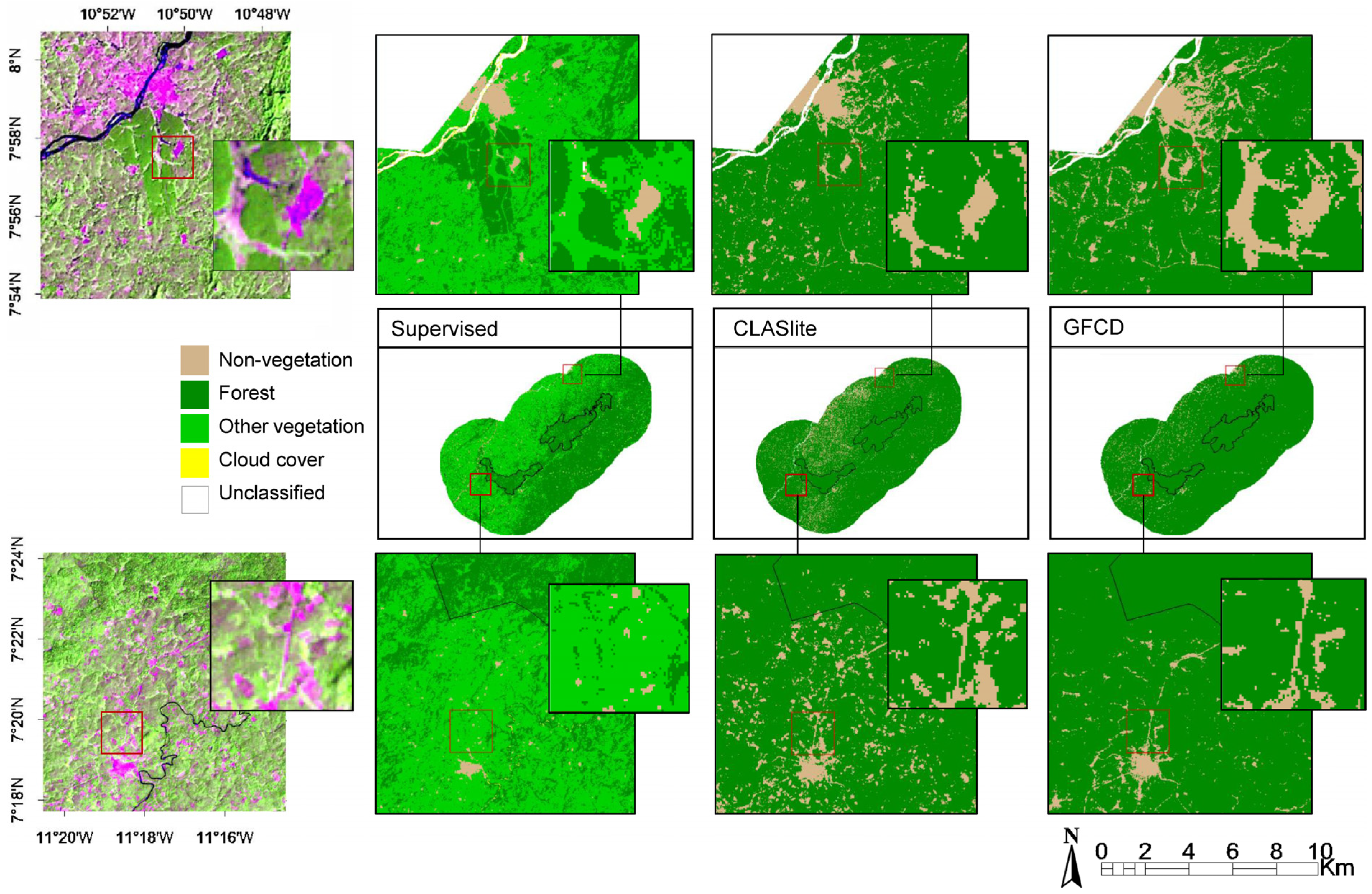
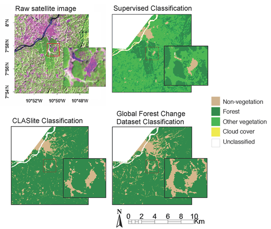
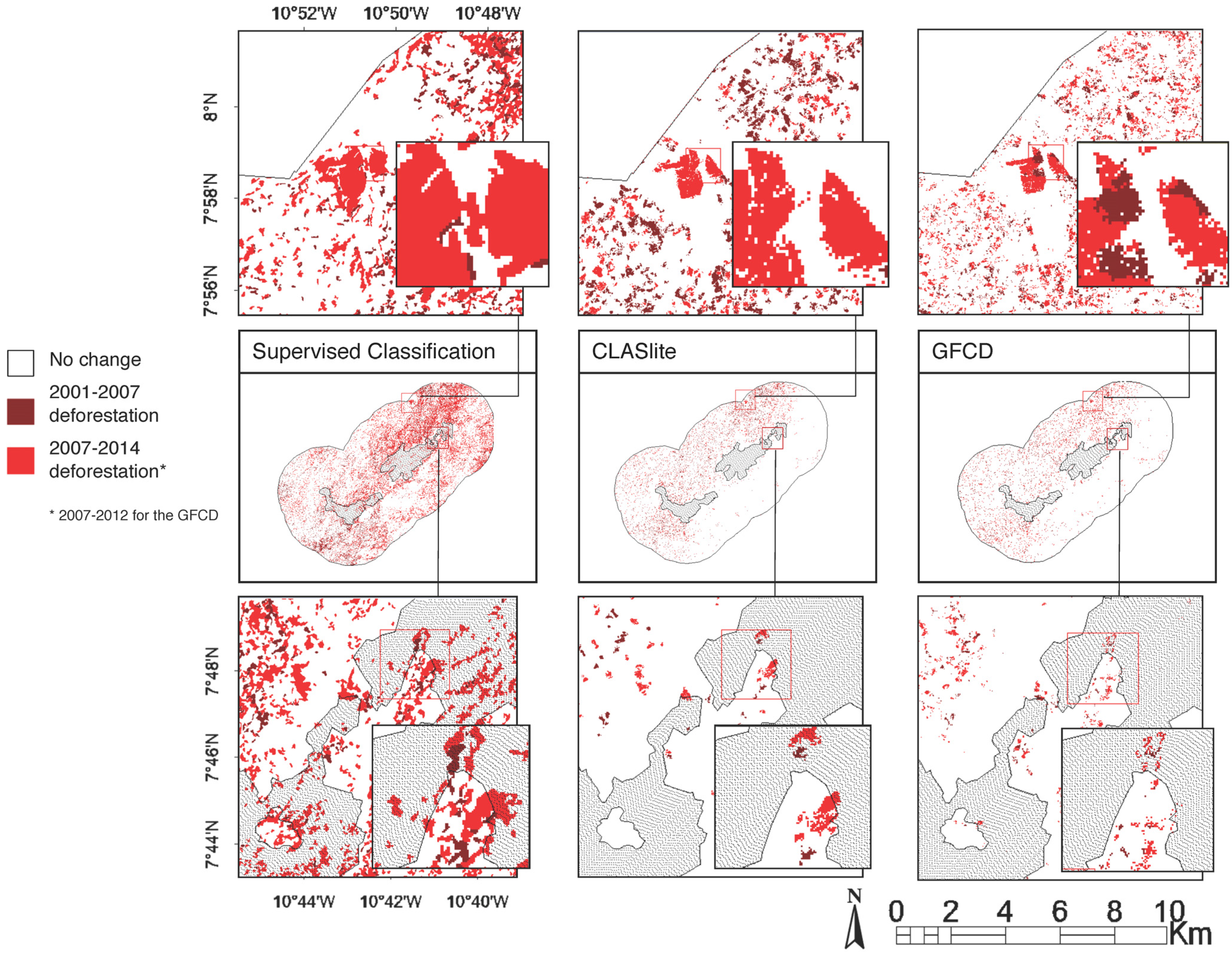
The land cover and change maps generated by the three distinct classification approaches over Gola and its surrounding region shared many similarities. Areas identified as having been deforested by all three approaches had a high degree of correspondence with true deforestation on the ground (see relatively high user’s accuracies for the deforestation categories, Table A4), indicating that the generated maps can serve as credible tools for tracking deforestation events. Direct visual interpretations of the change maps also offer useful preliminary insights into the spatial distributions of deforestation across the region. For instance, deforestation surrounding Gola since 2000 has been greater in Sierra Leone than in neighbouring Liberia to the immediate southeast (central panels of Figure 2), while all maps indicate the presence of encroachment across the boundary of Gola’s northern extension (bottom panels of Figure 2). Both of these findings can be used to inform the mobilisation of targeted ground-level conservation action in the region.
Critically, all three classification approaches employed in this study also exhibited difficulties in delineating anthropogenic from natural tree stands to some extent. At least 50% of other vegetation truth pixels were classified as forest by all three classification approaches, which influenced declines in the overall accuracies of the classified map products (Table 2, Table A3). We expected each of the classification approaches to exhibit at least some classification confusion surrounding this other vegetation class; as a catchment category of sorts for all vegetation other than mature natural forest, it encompassed a diverse array of vegetation types. We also expected this confusion because of known difficulties in using classification approaches based on information from optical sensors to distinguish mature natural forests from plantations, which may be spectrally similar to each other but structurally and functionally different. Still, remote sensing technologies that can distinguish natural forests from planted forests are of high value for conservationists. Thus, a primary aim of our study was to determine which classification approach employed here could best handle this classification challenge, and which of its unique features allowed it do so.
To this end, we found that, of the three classification tools employed in this study, CLASlite not only produced the most accurate land-cover and land cover-change products overall (Table 2, Table A4), but also was more adept at classifying other vegetation (inclusive of palm plantations and agricultural crop land) as non-forest rather than mature forest, especially in direct comparison with the GFCD (
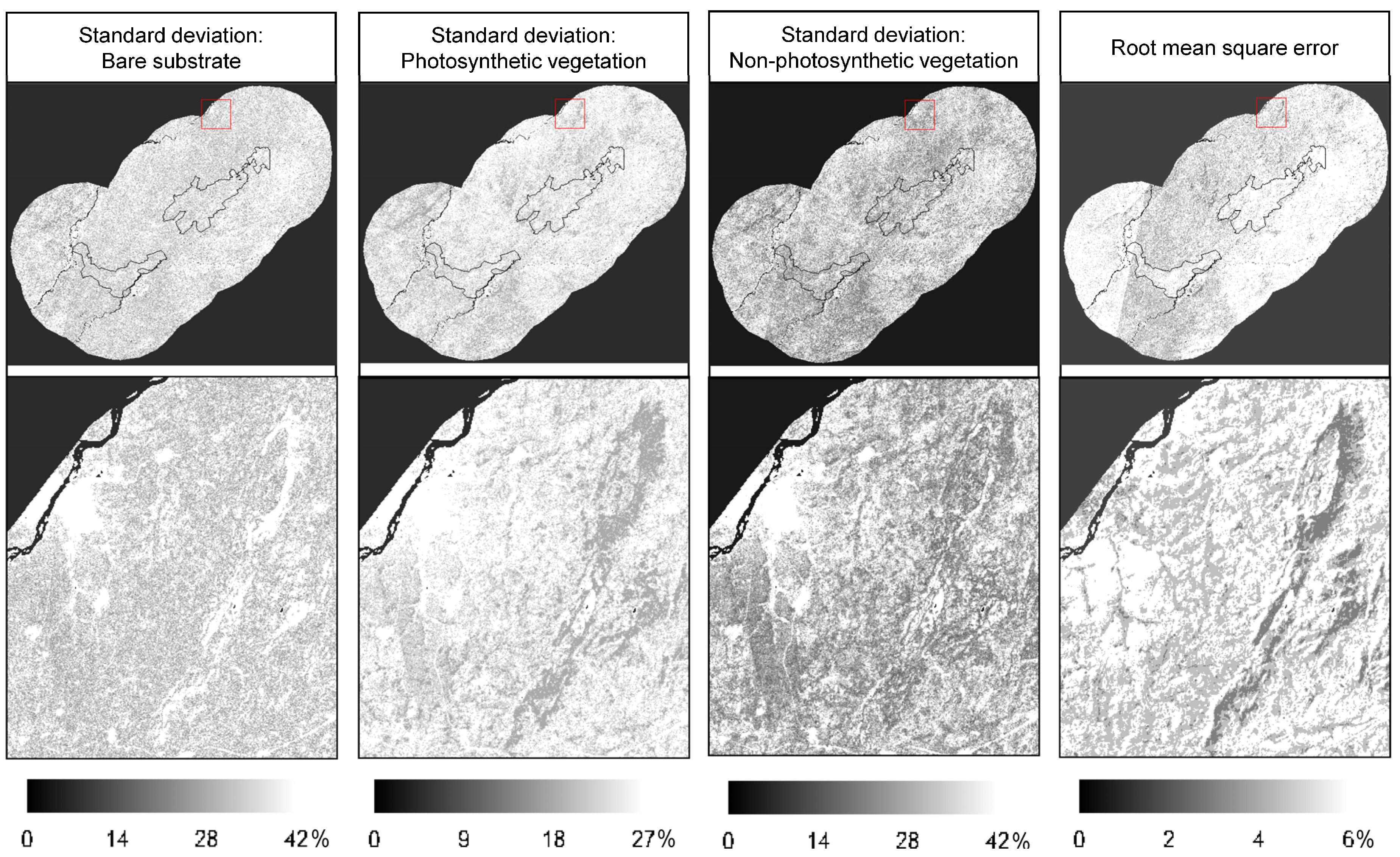
Table 2). Of the classification methodologies studied here, CLASlite featured the most robust sub-pixel analytical framework, an indication that the nature and extent of biophysical information that a classification method identifies at the sub-pixel level is a fundamental determinant of its capacity to discriminate planted from natural mature forest. CLASlite’s AutoMCU algorithm captures the sub-pixel spectral characteristics of an individual pixel by drawing from a vast spectral endmember library to first guess the reflectance spectra of three constituent endmembers (photosynthetic vegetation, non-photosynthetic vegetation, and bare substrate), and then assign fractional cover values to each of the three endmembers within the pixel (Figure A1(C)) [24]. In so doing, CLASlite attempts to account for the likelihood that each pixel has a heterogeneous composition, and consequent decisions on whether a pixel is interpreted as forest or non-forest are based on the degree to which the relative fractional covers of the pixel’s constituent endmembers meet certain user-defined thresholds. A previous study of forest degradation in Indonesian Borneo demonstrated that these thresholds can in fact be altered to exclude certain vegetation types (e.g., younger oil palm and timber plantations) from being classified by CLASlite as forest, as such plantations in the study area were found to be associated with pixels featuring greater percentages of bare substrate than pixels of natural forest [26]. Our study supports this claim that CLASlite’s more robust sub-pixel analytical approach is capable of discerning natural tree stands from planted tree stands—at least to a greater extent than the GFCD, and within the context of the Gola landscape.
In contrast, sub-pixel biophysical measurements were more limited in the GFCD product. Pixels in the GFCD dataset were considered at the sub-pixel level to the extent that a pixel was assigned a fractional tree cover endmember value from 0 to 1. However, we found that this percent tree cover-based definition of forest had limited success in discerning between natural and planted forest in this study; of the three classification approaches, the GFCD categorised the greatest percentage of other vegetation truth regions as forest (Table 2). Attempting to distinguish natural from planted forest based on tree cover can be problematic when plantations might feature tree cover extents that are comparable with that of natural forests. While this distinction is certainly not one of which the GFCD has claimed to be capable [56], it is still a limitation to the application of the GFCD in conservation studies that has been previously noted [57], and that our study corroborates. Although agreed-upon forest definitions in fact are commonly based on percent forest cover [30], our study indicates that such a discrete classification scheme, based on mutual exclusivity in which attempts are made to define natural forest by a single tree cover threshold, may not be particularly useful when attempting to differentiate natural from planted forests.
Supervised classification also utilised a sub-pixel analytical framework to a lesser extent than CLASlite, mirroring its more limited capacity to classify pixels that exist at the ambiguous boundaries of discrete land classes. The supervised classification approach employed here involved training a Maximum Likelihood classifier algorithm to first recognise particular spectral patterns as representative of certain user-defined land-cover classes of interest, then classify unknown pixels into one of the land-cover classes based on the likelihood of that pixel’s spectral signature falling within a normal distribution of the spectral values of a particular land class. Supervised classification’s binning of a pixel into one of several user-defined land classes based on overall spectral profile may fail to capture the more nuanced biophysical meaning behind a pixel, and such classification schemes may also substantially bypass land-change processes such as forest degradation that tend to be heterogeneous on finer, sub-pixel scales [58,59]. Moreover, dividing continuous quantitative information, such as those found in satellite images, into a finite number of discrete land classes that are considered at the outset to be exhaustively defined and mutually exclusive may lend itself to the further loss of information [60]. Such techniques may fail to accurately detect and separate “edge pixels,” for example, that exist near the spectral boundaries of different classes [16,61] as well as pixels that exhibit high reflectance variability [62]. An additional constraint can be imposed when spectral signals from the land area represented by a pixel are influenced by signals from immediately surrounding pixels [63]. These considerations are especially relevant to our study of the Gola landscape, which features a complex and spectrally diverse mosaic of forested and vegetated land having experienced varying degrees of disturbance and recovery [43].
Understanding the biophysical underpinnings of each classification methodology’s approach to sub-pixel measurements leads to an ontologically-based interpretation of CLASlite’s greater accuracy in classifying land cover and change over Gola when compared to the other approaches. Ontologies are agreements about shared conceptualisations [64], and ontological biases in remote sensing can arise from differences in the ways in which data terms are conceptualised, such that land-cover information becomes inherently relative and indeterminate [65]. Each of the three classification maps from this study was a product of different definitions of “forest” and, by extension, “non-forest.” “Forest” pixels in CLASlite were pixels that met user-assigned thresholds in photosynthetic vegetation and bare substrate fractional spectral signatures. The GFCD approach used in this study to generate forest-cover maps defined “forest” as pixels with >50% canopy closure for all vegetation taller than 5 m. Supervised classification defined forest as pixel clusters, separate in spectral space from other pixel clusters, that shared spectral similarities with a set of pre-assigned “truth” pixels representing forested areas in reality. Each of the classified products generated from this study and based on these diverse definitions of “forest” were subject to varying degrees of agreement errors with independently assigned truth pixels. However, CLASlite’s advantage stemmed from its encapsulation of a single pixel’s heterogeneity, allowing for an ontological interpretation of forest pixels that aligns most closely with the biophysical reality of naturally occurring phenomena often comprising spectra from more than one ground material [66]. Meanwhile, the GFCD’s more liberal ontology of what constitutes a forest has already been criticised for its conflation of tropical forests with monoculture plantations and even tall herbaceous crops [57]. Inconsistencies in land-cover nomenclature are broadly recognised as main barriers to forest monitoring strategies [67], and our exploration of how the technical differences among the classification techniques used in this study can be reinterpreted as ontological differences largely underscore this claim. Our study importantly illustrates that understanding the semantics of land-cover categories in any classification methodology is a critical prerequisite to understanding the nature of the land-cover products that can be derived from them.
Finally, it is likely that the relatively high flexibility in parameter setting afforded to the user by CLASlite allowed for the generation of a more superior classified map product over Gola. The GFCD is an already processed and packaged forest cover and change product. ENVI’s supervised classification approach, in contrast, allows for some degree of user input via the selection of the classifier algorithm (e.g., Maximum Likelihood, Minimum Distance, Mahalanobis Distance) used to assign individual pixels to land-cover categories, in addition to the setting of image “clean-up” parameters, which involved image smoothing (i.e., reclassifying pixels with the majority class value of their surrounding pixels to remove “salt-and-pepper” effects) and aggregation (i.e., merging very small and isolated pixel clusters with adjacent, larger regions). In fact, the CLASlite approach included similar image clean-up parameters in the form of artefact removal and pixel aggregation options (Table A2). The option of controlling the degree to which “salt-and-pepper” effects are removed as they pertain to a given study area can greatly influence the nature of the maps generated; by increasing edge densities and creating smaller blocks of any vegetation class [68], salt-and-pepper effects can contribute to the over-segmentation of an image [62], and thus reducing them through the use of filters [52,61,69] can reduce mis-registration errors [70]. However, among other parameter alterations, the CLASlite approach also critically allowed the user to define exact threshold levels for fractional photosynthetic vegetation and bare substrate values when determining forest cover (Table A2). Understandably, the option to define exactly what is considered forest and non-forest based on the local realities of a given study site facilitates the production of classified land cover and change maps that are better tailored to the area of interest.
Our study indicates that CLASlite’s analytical framework as is was able to best distinguish natural from planted tree stands over Gola. Thus, CLASlite as it stands has the potential to serve as a suitable remotely sensed data analysis tool for informing REDD, zero deforestation, high carbon stock forest, and other related policies that might rely upon this very distinction. However, it is important to consider the ways in which the accuracy metrics of the classified CLASlite product as well as the analytical capacities of the CLASlite technology itself can be further improved and extended. For example, it would be of interest to run a separate classifier on CLASlite’s intermediate fractional cover product to quantify threshold values for the three photosynthetic vegetation, non-photosynthetic vegetation, and bare substrate endmembers that would allow for the distinction of more land-cover classes beyond CLASlite’s forest/non-forest binary. Such analyses would certainly extend CLASlite’s capabilities of provisioning map products with even greater site relevance. More thorough interpretations of natural versus anthropogenic influences on forest cover and change might also be achieved by further classifying the forest cover and change CLASlite products based on factors that would likely influence human accessibility to forested areas, such as distance to roads, travel time from nearest city, and topographic features [25], or interpreting CLASlite products alongside remotely sensed radar data, which have been shown to discriminate oil palm plantations from forest stands with high accuracy [33]. Although the GFCD product as applied within the framework of our study was not the most optimal of the land-cover classification tools employed, the product itself still harbours opportunities for extended analyses as well. While the ramifications of the GFCD’s dependence on percent tree cover in defining forest have been explored (notably in [57]), it is perhaps the GFCD’s core identity as a percent tree cover product that lends itself to a wealth of extended and more tailored reinterpretations. For example, sensitivity analyses could be conducted to determine specific percent tree cover thresholds that would allow the GFCD product to distinguish certain vegetation types of interest given a particular landscape. Thus, the revolutionary powers of CLASlite and the GFCD as modern remote sensing technologies lie not only in the fact that they are free for public download and dissemination, and thus can empower vast groups of individuals to conduct informative forest monitoring research, but also in their status as compelling tools that offer vast opportunities for extended applications in a variety of contexts.

5. Limitations

Satellite imagery processing is a practice often riddled with biases and limitations, to the extent that extensively manipulated land-cover information is often, and erroneously, treated as land-cover data [71]. One limitation present in our analysis stems from differences in the acquisition dates of our satellite imagery. First, the end-date of Landsat imagery used in this study (from which the supervised classification and CLASlite products, as well as truthing pixels for accuracy assessment, were generated) was early 2014, while the GFCD product classified deforestation only to the end of 2012. The lack of temporal consistency between the Landsat imagery and the GFCD could have confounded absolute and relative accuracy assessments of the GFCD product and thus our confidence in it. Similarly, variations in land cover and change maps generated from this study could have been direct artefacts of differences in the original satellite imagery used, rather than solely the classification methodology employed. While the same base Landsat scenes of Gola’s dry season (during which cloud-free images were more prevalent) were used in both the supervised and CLASlite classification approaches, the GFCD was originally derived from computationally generated mosaics of cloud-free 30 m × 30 m Landsat pixels taken during the growing season. These differences in the fundamental nature of base satellite imagery used by the classification approaches in our work likely explain at least a portion of the differences in the generated maps. The sensitivity of the classification approaches used in this study to image acquisition time was particularly evident during the supervised classification exercise. Visual cross-comparisons of the regions that the supervised classification method classified as other vegetation within Gola’s administrative boundaries with previously published land-cover maps over Gola reveal the overlap of some of these areas with what has been identified by [48] as patches of semi-deciduous forest within Gola’s largely evergreen forest interior. Because the Landsat images used in this study were obtained from Gola’s dry season, which is coincident with the leaf-off condition of some semi-deciduous tree species of the region [72], it is likely that the supervised classification method was able to distinguish between the different spectral signatures of full-canopy evergreen trees from those of semi-deciduous trees that may have shed at least a portion of their foliage, resulting in relatively high estimates of non-forest vegetation cover where semi-deciduous trees exist. Finally, it is possible that limitations in the quality of “truth” pixels used in our study resulted in map biases. While we attempted to ensure the distribution of truth pixels across the region’s spatial extent through random placement and broadly adhered to truth pixel identification methodologies employed by previous peer-reviewed land-cover classification exercises of Gola, utilising ground-level truth data in our study might have afforded us more confidence in our accuracy assessments [35]. In particular, the sole use of high-resolution imagery to generate truth data may be liable to subjectivity arising from photo interpretation [73] as well as differences in filters applied to the image extent [74].

6. Conclusion

Given the array of new remotely sensed land-cover data, products, and analytical tools that are available—and still being developed—today, critical assessments of the relatively utility of these technologies for forest monitoring efforts are essential. Especially important for conservationists hoping to employ remote sensing tools is the need for technologies that can differentiate natural from planted mature forest. In this study, we explored the ways in which various definitions, assumptions, and algorithms inherent in three optical remote sensing-based land-classification methods, including two of the most recent technologies to have emerged in the field of remote sensing for forest monitoring, affected their land-cover and land cover-change classification abilities for a region of tropical forest in Sierra Leone, West Africa. We found that the CLASlite forest monitoring tool produced forest cover and change maps with greater quantified accuracies than a traditional supervised classification approach and one using the Global Forest Change dataset, and was able to also make the critical distinction between mature planted forest and mature natural forest to a greater extent than the other two approaches. The advantages of CLASlite largely derived from its ability to draw from a vast library of spectral endmembers to robustly resolve spectral signatures beyond the level of the discrete pixel, thus acknowledging the true spectral heterogeneity of forested areas, as well as its greater incorporation of user-defined parameter values. These factors afforded CLASlite the greater capacity to generate forest cover and change maps that held more local relevance than those derived from the other two classification approaches. Moreover, CLASlite features the additional benefit of encouraging a less centralised approach to forest monitoring by empowering conservation and resource policy communities with the tools necessary to perform this task themselves. Overall, by exploring the suite of land cover and change classification products that can result from applying various remote sensing tools for forest monitoring purposes, our study demonstrates the importance of process-oriented, rather than purely product-oriented, approaches to land classification. In other words, the mechanisms and processing chains utilised by various classification technologies, and the ways in which these differences materialise in generated map products, must be fully understood before remote sensing tools are applied to inform our understanding of ecological phenomena and conservation-related initiatives. Finally, we take this opportunity to emphasise the outstanding value in novel technologies such as CLASlite and the GFCD, both of which serve as robust, foundational tools with demonstrated and ever-growing capacities to advance the field of remote sensing for forest monitoring.

Acknowledgments

We thank the Keasbey Memorial Foundation for their funding of G.V.L.’s program of study at Cambridge. We thank Armando Apan (School of Civil Engineering and Surveying, University of Southern Queensland) and Beccy Wilebore (Department of Plant Sciences, University of Cambridge) for their help with ENVI software. D.A.C. benefited greatly from collaborations with the Royal Society for the Protection of Birds in Gola Rainforest National Park, funded by the Cambridge Conservation Initiative. We also thank Mark Mulligan (Department of Geography, King’s College London), Ed Tanner (Department of Plant Sciences, University of Cambridge), Will Simonson (Department of Plant Sciences, University of Cambridge), and three anonymous reviewers for their valuable and constructive comments and suggestions during the preparation of this manuscript.

Author Contributions

D.A.C. and G.V.L. collaborated in conceptualising the research plan and study methodology, interpreting the data, and editing the manuscript. D.A.C. supervised the work required for this paper. G.V.L. implemented the data acquisition and analysis, and prepared the manuscript.

Conflicts of Interest

The authors declare no conflict of interest. The founding sponsors had no role in the design of the study; in the collection, analyses, or interpretation of data; in the writing of the manuscript, and in the decision to publish the results.

References

  1. Kerr, J.T.; Ostrovsky, M. From space to species: Ecological applications for remote sensing. Trends Ecol. Evol. 2003, 18, 299–305. [Google Scholar] [CrossRef]
  2. Gross, J.E.; Goetz, S.J.; Cihlar, J. Application of remote sensing to parks and protected area monitoring: Introduction to the special issue. Remote Sens. Environ. 2009, 113, 1343–1345. [Google Scholar] [CrossRef]
  3. Wang, K.; Franklin, S.E.; Guo, X.; Cattet, M. Remote sensing of ecology, biodiversity and conservation: A review from the perspective of remote sensing specialists. Sensors 2010, 10, 9647–9667. [Google Scholar] [CrossRef] [PubMed]
  4. Nagendra, H.; Lucas, R.; Honrado, J.P.; Jongman, R.H.G.; Tarantino, C.; Adamo, M.; Mairota, P. Remote sensing for conservation monitoring: Assessing protected areas, habitat extent, habitat condition, species diversity, and threats. Ecol. Indic. 2013, 33, 45–59. [Google Scholar] [CrossRef]
  5. Woodcock, C.E.; Allen, A.A.; Anderson, M.; Belward, A.S.; Bindschadler, R.; Cohen, W.B.; Al., E. Free access to Landsat imagery. Science 2008, 320, 1011–1012. [Google Scholar] [CrossRef] [PubMed]
  6. Hansen, M.C.; Loveland, T.R. A review of large area monitoring of land cover change using Landsat data. Remote Sens. Environ. 2012, 122, 66–74. [Google Scholar] [CrossRef]
  7. Lefsky, M.A.; Cohen, W.B.; Parker, G.G.; Harding, D.J. Lidar remote sensing for ecosystem studies. BioScience 2002, 52, 19–30. [Google Scholar] [CrossRef]
  8. Asner, G.P.; Knapp, D.E.; Martin, R.E.; Tupayachi, R.; Anderson, C.B.; Mascaro, J.; Sinca, F.; Chadwick, K.D.; Higgins, M.; Farfan, W.; et al. Targeted carbon conservation at national scales with high-resolution monitoring. Proc. Natl. Acad. Sci. U.S.A. 2014, 111, E5016–E5022. [Google Scholar] [CrossRef] [PubMed]
  9. Asner, G.P.; Mascaro, J.; Muller-Landau, H.C.; Vieilledent, G.; Vaudry, R.; Rasamoelina, M.; Hall, J.S.; van Breugel, M. A universal airborne LiDAR approach for tropical forest carbon mapping. Oecologia 2012, 168, 1147–1160. [Google Scholar] [CrossRef] [PubMed]
  10. Goetz, S.; Dubayah, R. Advances in remote sensing technology and implications for measuring and monitoring forest carbon stocks and change. Carbon Manag. 2011, 2, 231–244. [Google Scholar] [CrossRef]
  11. Lamonaca, A.; Corona, P.; Barbati, A. Exploring forest structural complexity by multi-scale segmentation of VHR imagery. Remote Sens. Environ. 2008, 112, 2839–2849. [Google Scholar] [CrossRef] [Green Version]
  12. Kayitakire, F.; Hamel, C.; Defourny, P. Retrieving forest structure variables based on image texture analysis and IKONOS-2 imagery. Remote Sens. Environ. 2006, 102, 390–401. [Google Scholar] [CrossRef]
  13. Beguet, B.; Guyon, D.; Boukir, S.; Chehata, N. Automated retrieval of forest structure variables based on multi-scale texture analysis of VHR satellite imagery. ISPRS J. Photogramm. Remote Sens. 2014, 96, 164–178. [Google Scholar] [CrossRef]
  14. Kim, D.; Sexton, J.O.; Noojipady, P.; Huang, C.; Anand, A.; Channan, S.; Feng, M.; Townshend, J.R. Remote Sensing of Environment Global, Landsat-based forest-cover change from 1990 to 2000. Remote Sens. Environ. 2014, 155, 178–193. [Google Scholar] [CrossRef]
  15. Turner, W.; Spector, S.; Gardiner, N.; Fladeland, M.; Sterling, E.; Steininger, M. Remote sensing for biodiversity science and conservation. Trends Ecol. Evol. 2003, 18, 306–314. [Google Scholar] [CrossRef]
  16. Kennedy, R.E.; Townsend, P.; Gross, J.E.; Cohen, W.B.; Bolstad, P.; Wang, Y.Q.; Adams, P. Remote sensing change detection tools for natural resource managers: Understanding concepts and tradeoffs in the design of landscape monitoring projects. Remote Sens. Environ. 2009, 113, 1382–1396. [Google Scholar] [CrossRef]
  17. Leidner, A.K.; Turner, W.; Pettorelli, N.; Leimgruber, P.; Wegmann, M. Satellite remote sensing for biodiversity research and conservation applications. In Proceedings of Committee on Earth Observation Satellites (CEOS) Workshop, Munich, Germany, 8–10 October 2012; pp. 1–26.
  18. Corbane, C.; Lang, S.; Pipkins, K.; Alleaume, S.; Deshayes, M.; García Millán, V.E.; Strasser, T.; Vanden Borre, J.; Toon, S.; Michael, F. Remote sensing for mapping natural habitats and their conservation status—New opportunities and challenges. Int. J. Appl. Earth Obs. Geoinf. 2015, 37, 7–16. [Google Scholar] [CrossRef]
  19. Wiens, J.; Sutter, R.; Anderson, M.; Blanchard, J.; Barnett, A.; Aguilar-Amuchastegui, N.; Avery, C.; Laine, S. Selecting and conserving lands for biodiversity: The role of remote sensing. Remote Sens. Environ. 2009, 113, 1370–1381. [Google Scholar] [CrossRef]
  20. Lang, S.; Mairota, P.; Pernkopf, L.; Schioppa, E.P. Earth observation for habitat mapping and biodiversity monitoring. Inter. J. Appl. Earth Obs. Geoinf. 2015, 37, 1–6. [Google Scholar] [CrossRef]
  21. Asner, G.P.; Keller, M.; Pereira, R.; Zweede, J.C.; Silva, J.N. Canopy damage and recovery after selective logging in Amazonia: Field and satellite studies. Ecol. Appl. 2004, 14, S280–S298. [Google Scholar] [CrossRef]
  22. Peres, C.A.; Barlow, J.; Laurance, W.F. Detecting anthropogenic disturbance in tropical forests. Trends Ecol. Evol. 2006, 21, 227–9. [Google Scholar] [CrossRef] [PubMed]
  23. Asner, G.P. Satellites and psychology for improved forest monitoring. Proc. Natl. Acad. Sci. U.S.A. 2014, 111, 567–568. [Google Scholar] [CrossRef] [PubMed]
  24. Asner, G.P.; Tasar, E.; Sousan, S.; Knapp, D. CLASlite Forest Monitoring Technology: Version 3.1 User Guide; Carnegie Institution for Science Department of Global Ecology: Stanford, CA, USA, 2013. [Google Scholar]
  25. Allnutt, T.F.; Asner, G.P.; Golden, C.D.; Powell, G.V.N. Mapping recent deforestation and forest disturbance in northeastern Madagascar. Trop. Conserv. Sci. 2013, 6, 1–15. [Google Scholar]
  26. Bryan, J.E.; Shearman, P.L.; Asner, G.P.; Knapp, D.E.; Aoro, G.; Lokes, B. Extreme differences in forest degradation in Borneo: Comparing practices in Sarawak, Sabah, and Brunei. PLoS ONE 2013, 8, e69679. [Google Scholar] [CrossRef] [PubMed]
  27. Hansen, M.C.; Potapov, P.; Moore, R.; Hancher, M.; Turubanova, S.; Tyukavina, A.; Thau, D.; Stehman, S. V; Goetz, S.J.; Loveland, T.R.; et al. High-resolution global maps of 21st-century forest cover change. Science 2013, 342, 850–853. [Google Scholar] [CrossRef]
  28. World Resources Institute. Global forest watch. In World Resources Institute Annual Review; World Resources Institute: Washington, DC, USA, 2002; pp. 20–21. [Google Scholar]
  29. Tsendbazar, N.E.; de Bruin, S.; Herold, M. Assessing global land cover reference datasets for different user communities. ISPRS J. Photogramm. Remote Sens. 2014. [Google Scholar] [CrossRef]
  30. Brown, S.; Zarin, D. What does zero deforestation mean? Science 2013, 342, 805–807. [Google Scholar] [CrossRef] [PubMed]
  31. Senf, C.; Pflugmacher, D.; van der Linden, S.; Hostert, P. Mapping rubber plantations and natural forests in Xishuangbanna (Southwest China) using multi-spectral phenological metrics from modis time series. Remote Sens. 2013, 5, 2795–2812. [Google Scholar] [CrossRef]
  32. Li, Z.; Fox, J.M. Mapping rubber tree growth in mainland Southeast Asia using time-series MODIS 250 m NDVI and statistical data. Appl. Geogr. 2012, 32, 420–432. [Google Scholar] [CrossRef]
  33. Morel, A.C.; Saatchi, S.S.; Malhi, Y.; Berry, N.J.; Banin, L.; Burslem, D.; Nilus, R.; Ong, R.C. Estimating aboveground biomass in forest and oil palm plantation in Sabah, Malaysian Borneo using ALOS PALSAR data. Forest Ecol. Manag. 2011, 262, 1786–1798. [Google Scholar] [CrossRef]
  34. Griscom, B.W.; Cortez, R. The case for improved forest management (IFM) as a priority REDD+ strategy in the tropics. Trop. Conserv. Sci. 2013, 6, 409–425. [Google Scholar]
  35. Horning, N. Land Cover Classification Methods, Version 1.0; American Museum of Natural History, Center for Biodiversity and Conservation: New York, NY, USA, 2004. [Google Scholar]
  36. Johnson, B.; Xie, Z. Unsupervised image segmentation evaluation and refinement using a multi-scale approach. ISPRS J. Photogramm. Remote Sens. 2011, 66, 473–483. [Google Scholar] [CrossRef]
  37. McDermid, G.J.; Franklin, S.E.; LeDrew, E.F. Remote sensing for large-area habitat mapping. Progr. Phys. Geogr. 2005, 29, 449–474. [Google Scholar] [CrossRef]
  38. Cleve, C.; Kelly, M.; Kearns, F.R.; Moritz, M. Classification of the wildland-urban interface: A comparison of pixel- and object-based classifications using high-resolution aerial photography. Comput. Environ. Urban Systems 2008, 32, 317–326. [Google Scholar] [CrossRef]
  39. Blaschke, T. Object based image analysis for remote sensing. ISPRS J. Photogramm. Remote Sens. 2010, 65, 2–16. [Google Scholar] [CrossRef]
  40. Hussain, M.; Chen, D.; Cheng, A.; Wei, H.; Stanley, D. Change detection from remotely sensed images: From pixel-based to object-based approaches. ISPRS J. Photogramm. Remote Sens. 2013, 80, 91–106. [Google Scholar] [CrossRef]
  41. Horning, N.; Robinson, J.A.; Sterling, E.J.; Turner, W.; Spector, S. Remote sensing for Ecology and Conservation: A Handbook of Techniques; Oxford University Press Inc.: New York, NY, USA, 2010. [Google Scholar]
  42. Zhang, H.; Fritts, J.E.; Goldman, S.A. Image segmentation evaluation: A survey of unsupervised methods. Comput. Vision Image Underst. 2008, 110, 260–280. [Google Scholar] [CrossRef]
  43. Lindsell, J.A.; Klop, E. Spatial and temporal variation of carbon stocks in a lowland tropical forest in West Africa. Forest Ecol. Manag. 2013, 289, 10–17. [Google Scholar] [CrossRef]
  44. The Royal Society for the Protection of Birds. In The Gola REDD Project; The Climate, Community and Biodiversity Alliance: Washington, DC, USA, 2013; pp. 11–140.
  45. Lindsell, J.A.; Klop, E.; Siaka, A.M. The impact of civil war on forest wildlife in West Africa: Mammals in Gola Forest, Sierra Leone. Oryx 2011, 45, 69–77. [Google Scholar] [CrossRef]
  46. Sowa, S.S. Proposed network of protected areas. In National Data Collection Report: Sierra Leone; United Nations Environment Programme World Conservation Monitoring Centre: Cambridge, UK, 2012; pp. 7–39. [Google Scholar]
  47. Klop, E.; Lindsell, J.; Siaka, A. Biodiversity of Gola Forest, Sierra Leone; Royal Society for the Protection of Birds: Sandy, UK, 2008. [Google Scholar]
  48. Vaglio Laurin, G.; Liesenberg, V.; Chen, Q.; Guerriero, L.; Del Frate, F.; Bartolini, A.; Coomes, D.; Wilebore, B.; Lindsell, J.; Valentini, R. Optical and SAR sensor synergies for forest and land cover mapping in a tropical site in West Africa. Inter. J. Appl. Earth Obs. Geoinf. 2013, 21, 7–16. [Google Scholar] [CrossRef]
  49. USGS Global Visualization Viewer. Available online: http://glovis.usgs.gov (accessed on 4 December 2013).
  50. Townsend, P.A.; Lookingbill, T.R.; Kingdon, C.C.; Gardner, R.H. Spatial pattern analysis for monitoring protected areas. Remote Sens. Environ. 2009, 113, 1410–1420. [Google Scholar] [CrossRef]
  51. Giri, C.; Pengra, B.; Long, J.; Loveland, T.R. Next generation of global land cover characterization, mapping, and monitoring. Inter. J. Appl. Earth Obs. Geoinf. 2013, 25, 30–37. [Google Scholar] [CrossRef]
  52. Otukei, J.R.; Blaschke, T. Land cover change assessment using decision trees, support vector machines and maximum likelihood classification algorithms. Int. J. Appl. Earth Obs. Geoinf. 2010, 12, S27–S31. [Google Scholar] [CrossRef]
  53. Churches, C.E.; Wampler, P.J.; Sun, W.; Smith, A.J. Evaluation of forest cover estimates for Haiti using supervised classification of Landsat data. Int. J. Appl. Earth Obs. Geoinf. 2014, 30, 203–216. [Google Scholar] [CrossRef]
  54. Global Forest Change 2000-2012 Data Download. Available online: http://earthenginepartners.appspot.com/science-2013-global-forest/download.html (accessed on 3 March 2014).
  55. Congalton, R.G. A review of assessing the accuracy of classifications of remotely sensed data. Remote Sens. Environ. 1991, 37, 35–46. [Google Scholar] [CrossRef]
  56. Hansen, M.C.; Potapov, P.; Margono, B.; Stehman, S.; Turubanova, S.; Tyukavina, A. Response to comment on “High-resolution global maps of 21st-century forest cover change”. Science 2014, 344, 981. [Google Scholar] [CrossRef] [PubMed]
  57. Tropek, R.; Sedláček, O.; Beck, J.; Keil, P.; Musilová, Z.; Símová, I.; Storch, D. Comment on “High-resolution global maps of 21st-century forest cover change”. Science 2014, 344, 981. [Google Scholar] [CrossRef] [PubMed]
  58. Asner, G.P.; Knapp, D.E.; Balaji, A.; Paez-Acosta, G. Automated mapping of tropical deforestation and forest degradation: CLASlite. J. Appl. Remote Sens. 2009, 3, 033543. [Google Scholar] [CrossRef]
  59. Ellis, E.C.; Wang, H.; Xiao, H.S.; Peng, K.; Liu, X.P.; Li, S.C.; Ouyang, H.; Cheng, X.; Yang, L.Z. Measuring long-term ecological changes in densely populated landscapes using current and historical high resolution imagery. Remote Sens. Environ. 2006, 100, 457–473. [Google Scholar] [CrossRef]
  60. Rocchini, D.; Foody, G.M.; Nagendra, H.; Ricotta, C.; Anand, M.; He, K.S.; Amici, V.; Kleinschmit, B.; Förster, M.; Schmidtlein, S.; et al. Uncertainty in ecosystem mapping by remote sensing. Comput. Geosci. 2013, 50, 128–135. [Google Scholar] [CrossRef]
  61. Hester, D.B.; Cakir, H.I.; Nelson, S.A.C.; Khorram, S. Per-pixel classification of high spatial resolution satellite imagery for urban land-cover mapping. Photogramm. Eng. Remote Sens. 2008, 74, 463–471. [Google Scholar] [CrossRef]
  62. Carleer, A.P.; Debeir, O.; Wolff, E. Assessment of very high spatial resolution satellite image segmentations. Photogramm. Eng. Remote Sens. 2005, 71, 1285–1294. [Google Scholar] [CrossRef]
  63. Townshend, J.R.G.; Huang, C.; Kalluri, S.N.V.; Defries, R.S.; Liang, S.; Yang, K. Beware of per-pixel characterization of land cover. Inter. J. Remote Sens. 2000, 21, 839–843. [Google Scholar] [CrossRef]
  64. Câmara, G.; Egenhofer, M.J.; Fonseca, F.; Miguel, A.; Monteiro, V. What’s in an image? In Spatial Information Theory—Foundations of Geographic Information Science; Montello, D.R., Ed.; Springer-Verlag: Berlin, Germany, 2001; pp. 474–488. [Google Scholar]
  65. Comber, A.; Fisher, P.; Wadsworth, R. You know what land cover is but does anyone else? An investigation into semantic and ontological confusion. Inter. J. Remote Sens. 2005, 26, 223–238. [Google Scholar] [CrossRef]
  66. Ji, M.; Feng, J. Subpixel measurement of mangrove canopy closure via spectral mixture analysis. Front. Earth Sci. 2011, 5, 130–137. [Google Scholar] [CrossRef]
  67. Verburg, P.H.; Neumann, K.; Nol, L. Challenges in using land use and land cover data for global change studies. Global Change Biol. 2011, 17, 974–989. [Google Scholar] [CrossRef]
  68. Fassnacht, K.S.; Cohen, W.B.; Spies, T.A. Key issues in making and using satellite-based maps in ecology: A primer. Forest Ecol. Manag. 2006, 222, 167–181. [Google Scholar] [CrossRef]
  69. Blaschke, T.; Lang, S.; Lorup, E.; Strobl, J.; Zeil, P. Object-oriented image processing in an integrated GIS/remote sensing environment and perspectives for environmental applications. Environ. Inf. Plan. Polit. Public 2000, 2, 555–570. [Google Scholar]
  70. Rogan, J.; Franklin, J.; Roberts, D.A. A comparison of methods for monitoring multitemporal vegetation change using Thematic Mapper imagery. Remote Sens. Environ. 2002, 80, 143–156. [Google Scholar] [CrossRef]
  71. Comber, A.; Fisher, P.; Wadsworth, R. Comparing statistical and semantic approaches for identifying change from land cover datasets. J. Environ. Manag. 2005, 77, 47–55. [Google Scholar] [CrossRef]
  72. Vaglio Laurin, G.; Chen, Q.; Lindsell, J.A.; Coomes, D.A.; Frate, F. Del; Guerriero, L.; Pirotti, F.; Valentini, R. Above ground biomass estimation in an African tropical forest with lidar and hyperspectral data. ISPRS J. Photogramm. Remote Sens. 2014, 89, 49–58. [Google Scholar] [CrossRef]
  73. Hill, T.B. Taking the “ ” out of “ground truth”: Objective accuracy assessment. In Proceedings of the 12th Pecora Conference, Sioux Falls, SD, USA, 24–26 August 1993.
  74. Castilla, G.; Hay, G.J. Uncertainties in land use data. Hydrol. Earth Syst. Sci. 2007, 11, 1857–1868. [Google Scholar] [CrossRef]

Appendix

Figure A1. Intermediate products derived from each of CLASlite’s four built-in steps using the 2014 Landsat satellite image over the eastern portion of Gola as an example. (A) Band selection for representation of the raw Landsat image is R = Band 5 (0.85–0.88 μm), G = Band 4 (0.64–0.67 μm), and B = Band 3 (0.53–0.59 μm). (B) Band selection for representation of the reflectance product is the same as that for (A). (C) Band selection for representation of the fractional cover product is R = bare substrate, G = photosynthetic vegetation, B = non-photosynthetic vegetation. (D) In forest cover product, grey areas represent forested regions and white areas represent non-forested regions. The Gola National Park boundary is outlined in either red or orange, while the extent of the 25 km boundary surrounding Gola is depicted in blue.
Remotesensing 07 02781 g003
Table A1. Supporting information for Landsat satellite images acquired over Gola used in this study. “East” and “West” locations refer to images acquired from the eastern and western portion of Gola. “ETM+” refers to the Enhanced Thematic Mapper Plus sensor, “TM” to the Thematic Mapper sensor, and “OLI-TIRS” to the Operational Land Image-Thermal Infrared sensor.
YearLocationPath/RowImage Acquisition DateSatelliteSensorCloud Cover (%)
2001East200/0557 February 2001Landsat 7 ETM+0.00
West201/05529 January 2001Landsat 7 ETM+4.00
2007East200/05515 January 2007Landsat 5TM0.00
West201/0556 January 2007Landsat 5TM0.00
2014East200/0553 February 2014Landsat 8 OLI-TIRS1.71
West201/0559 January 2014Landsat 8 OLI-TIRS9.44
Table A2. Summary of parameter change decisions while classifying each of the six Landsat images over Gola in the Carnegie Landsat Analysis System lite (CLASlite) version 3.1. Numbers before each parameter refer to the CLASlite step during which the option to alter the parameter was offered: 1 = raw image to reflectance, 2 = reflectance to fractional cover, 3 = fractional cover to forest cover, and 4 = forest cover to forest-cover change. “East” and “West” Landsat scene descriptors refer to the eastern and western portions of Gola, respectively.
Landsat scene
Parameter and parameter function2001 West2001 East2007 West2007 East2014 West2014 EastNotes
1. Masking: To mask clouds and water.ReducedDefault masking acceptedReducedReducedDefault masking acceptedDefault masking acceptedMasking was reduced in instances where CLASlite was erroneously masking water and cloud shadow.
2. Masking extent (%): To mask clouds and water.94949594094Default masking extent of 93% was not accepted for any images in order to balance water body masking with the preservation of terrestrial land.
3. Substrate (S) and photosynthetic vegetation (PV) threshold values: To define classes of forest and non-forest from sub-pixel fractional cover map.22 S, 80 PV22 S, 78 PV20 S, 80 PV (default)18 S, 76 PV20 S, 85 PV15 S, 80 PVFor each scene, S and PV thresholds were chosen in an attempt to most accurately distinguish forest from non-forest.
4. Percentage of deforestation (defor) and disturbance (dist) artefacts removed: To remove isolated deforestation and degradation pixels from maps, recognising that such events rarely happen in isolation. Defor: 50, Dist: 25 (default)Defor: 50, Dist: 25 (default)Defor: 50, Dist: 25 (default)Defor: 50, Dist: 25 (default)Defor: 50, Dist: 25 (default)Defor: 50, Dist: 25 (default)
4. Aggregation feature: To add to the deforestation map disturbance pixels in close proximity to other deforestation events, recognising that disturbance pixels are generally associated with the same forest-loss events. On (default)On (default)On (default)On (default)On (default)On (default)
Figure A2. Uncertainty of the bare substrate (S), photosynthetic vegetation (PV), and non-photosynthetic vegetation (NPV) fractional cover outputs from CLASlite alongside total error (root mean square error) of CLASlite’s fractional cover output over the 25 km region surrounding Gola. Error images derive from the 2014 Landsat image over the eastern portion of Gola. Standard deviations of CLASlite’s AutoMCU iterations represent the uncertainties of the S, PV, and NPV outputs. The root mean square error of the modelled versus observed reflectance signatures expresses total map error. Zoomed-in areas of the regions enclosed by red squares in the top row of panels appear in the bottom row of panels and represent the same palm plantation depicted in the top row of Figure 1 and Figure 2. The Gola National Park boundary is outlined in black.
Remotesensing 07 02781 g004
Table A3. Contingency matrix assessing the accuracy of the land-classification map of Gola and its surrounding 25 km region in early 2001 derived from supervised classification in ENVI. The three truth classes (in rows) are compared pair-wise with the three land-cover classes of the classification image (in columns). Values in the “Truth Class” rows represent percentage of total pixels in the truth class classified as a given land-cover type on the derived land-cover maps, with 2960 total pixels identified in the mature forest truth class, 2522 total pixels in the other vegetation class, and 2776 total pixels in the non-vegetation truth class. All accuracy values are presented as percentages. Kappa coefficient is reported ± one standard error.
Classification Map Land-Cover Type
Mature Forest Other Vegetation Non-Vegetation
Truth Class 1: Mature forest 91.38.70
Truth Class 2: Other vegetation 50.745.63.7
Truth Class 3: Non-vegetation08.991.1
User’s accuracy68.069.596.4
Producer’s accuracy91.345.691.1
Overall accuracy77.3
Kappa coefficient 0.66 ± 0.007
Table A4. Contingency matrices assessing the accuracy of the three forest cover-change maps of Gola and its surrounding 25 km region from 2001–2007 and 2007–2014* derived from supervised classification in ENVI, classification in the Carnegie Landsat Analysis System lite (CLASlite), and classification from the Global Forest Change dataset (GFCD). Values in the “Truth Class” rows represent percentage of total pixels from the truth class classified into deforestation or no change on the derived maps. For the 2001–2007 change maps, 3471 total pixels were identified in the deforestation truth class and 3265 total pixels were identified in the no change truth class. For the 2007–2014 change maps, 4004 total pixels were identified in the no change truth class and 3159 total pixels were identified in the deforestation truth class. All accuracy values are presented as percentages. Kappa coefficients are reported ± one standard error.
Supervised CLASlite GFCD
DeforestationNo Change DeforestationNo Change DeforestationNo Change
2001–2007Truth Class 1: Deforestation35.164.9 59.540.5 19.880.2
Truth Class 2: No change1.498.6 0100 0.199.9
User’s accuracy96.358.8 10069.8 99.753.7
Producer’s accuracy35.198.6 59.5100 19.899.9
Overall accuracy65.8 79.1 58.4
Kappa coefficient0.32 ± 0.009 0.59 ± 0.009 0.19 ± 0.007
2007–2014*Truth Class 1: Deforestation51.148.9 76.523.5 7.792.3
Truth Class 2: No change5.794.3 0100 0.199.9
User’s accuracy87.771.0 10084.3 98.757.5
Producer’s accuracy51.194.3 76.5100 7.799.9
Overall accuracy75.3 89.6 58.9
Kappa coefficient0.48 ± 0.01 0.78 ± 0.007 0.083 ± 0.005
* Note that the end date for the GFCD product only was the end of 2012.

