Normalization of Echo Features Derived from Full-Waveform Airborne Laser Scanning Data

Abstract

Full-waveform airborne laser scanning systems provide fundamental observations for each echo, such as the echo width and amplitude. Geometric and physical information about illuminated surfaces are simultaneously provided by a single scanner. However, there are concerns about whether the physical meaning of observations is consistent among different scanning missions. Prior to the application of waveform features for multi-temporal data classification, such features must be normalized. This study investigates the transferability of normalized waveform features to different surveys. The backscatter coefficient is considered to be a normalized physical feature. A normalization process for the echo width, which is a geometric feature, is proposed. The process is based on the coefficient of variation of the echo widths in a defined neighborhood, for which the Fuzzy Small membership function is applied. The normalized features over various land cover types and flight missions are investigated. The effects of different feature combinations on the classification accuracy are analyzed. The overall accuracy of the combination of normalized features and height-based attributes achieves promising results (>93% overall accuracy for ground, roof, low vegetation, and tree canopy) when different flight missions and classifiers are used. Nevertheless, the combination of all possible features, including raw features, normalized features, and height-based features, performs less well and yields inconsistent results.

1. Introduction

Land cover changes on Earth have become increasingly important. The need for better land cover information extends to local, national and global levels. With rapid advancements in remote sensing, it is relatively inexpensive to acquire up-to-date information over large geographical areas. Integration of features from multisource or multi-temporal data has become popular. Feature selection plays a crucial role in any image analysis process that uses remotely sensed data. It is often assumed that incorporation of additional features should enhance the accuracy of classification. Nevertheless, critical issues regarding the consistency of features with physical units remain. Scientists who are interested in land cover changes would like to study the characteristics of the “target” over time, rather than variations derived from remotely sensed data that are due to factors, such as the viewing angle, atmospheric conditions, topography, and viewing distance. Therefore, either relative or absolute calibration of spectral images is often implemented.

Airborne laser scanning (ALS) technology is an active remote sensing technique that produces a true orthophoto at a single wavelength. No sunlight is required, and there is less dependence on weather compared with other methods. Small-footprint full-waveform ALS systems that store the entire waveform of each received pulse have become available within the commercial sector. There has been great interest in maximizing the potential of waveform data. Compared with traditional discrete-return systems, more details about illuminated targets are stored in the waveform. The waveform contains information about surface characteristics, which may help identify surface features. Additionally, obtaining simultaneous geometric and physical information should be possible with a single ALS system.

Over the past decade, there has been a dramatic increase in the development of off-terrain filtering or object detection algorithms that rely strongly on the spatial relationship between 3D ALS points in their pursuit of automated processing [1,2]. Typical discrete-return systems provide intensity values for the physical information of each return; however, such information is too noisy to be used for interpretation of point clouds. Such information is rarely used because of its strong variability as a function of different factors. For example, the intensity value, which should yield the reflectance of the intercepting surface, can be affected by the footprint size, scan angle, range and backscatter cross-section of each echo [3]. Returns alone provide insufficient information about the characteristics of the illuminated surface and, without ancillary imagery, the task of interpreting points presents a considerable challenge [4]. To separate buildings, trees, and grass-covered areas, optical and multi-spectral imagery are often incorporated with discrete ALS data. Alternatively, intensity correction or normalization must be applied to reduce intensity variation if a meaningful comparison is to be made between multiple intensity datasets. Höfle and Pfeifer [5] developed two correction methods, data- and model-driven methods, to reduce the intensity variation for surface classification and multi-temporal analysis. A reduction of up to 2/7 of the original variation and significant global adjustment of the single flight strips was achieved. Nevertheless, special requirements for flight campaigns and a number of assumptions about system parameters are needed for these approaches to work. It is noted that the peak amplitude and echo width extracted from full-waveform data can be employed to calculate the target reflectance ρ with fewer assumptions regarding the system parameters [5].

In terms of extracting physical features from full-waveform data, two main observations (the width and amplitude) and derivatives (the backscatter cross-section and backscattering coefficient) are often investigated [6,7,8]. Jutzi and Gross [9] demonstrated the influence of the incidence angle and range on the echo amplitude variation. Abed et al. [10] developed a robust estimate of the incidence angle to compensate for the effect of the incidence angle on the echo amplitude. Additionally, those authors suggested that such a correction could be applied to other physical echo parameters, such as the backscatter cross-section and backscatter coefficient. Alexander et al. [6] found that the backscatter coefficient is more useful than the amplitude and backscatter cross-section for discriminating road and grass. On the other hand, a geometric waveform feature known as the echo width plays an important role in 3D vegetation mapping and terrain classification [9,11]. However, Guo et al. [12] concluded that the echo width values are too noisy to discriminate among the four classes investigated (building, vegetation, cement ground and natural ground types). Lin et al. [13] found that the echo width of an individual ALS point could be significantly affected by the flight altitude at a specified significance level (α) = 0.05; nevertheless, the standard deviation of the echo widths in the neighborhood was not influenced by the flight altitude in a statistical sense. They suggested that it might be better to apply the echo width information in a defined neighborhood when treating datasets acquired from various scan geometries and flight altitudes. In ALS data processing, the normalization process is usually applied to physical or radiometric features, such as the intensity, amplitude and backscatter cross-section. Investigations into the normalization of geometric features such as the echo width are rare. Geometric and physical information about illuminated surfaces are simultaneously provided by a single laser scanning system. However, there are concerns about whether the physical meaning of observations is consistent among different scanning missions.

Therefore, this study aims to normalize the waveform features to make the features more transferrable between the same or different flight missions. In addition, the impact of various feature combinations created with two classifiers, decision tree (DT) and neural network (NN) classifiers, on the accuracy of classification is investigated. The influence of raw waveform features, normalized waveform features or height-based features on the classification results is investigated. This analysis demonstrates how much non-normalized features may degrade the results of classification.

2. Methodology

2.1. Background

Waveform systems record the time history of the return signal from an individual laser shot, which represents the sum of reflections from all intercepted surfaces within the footprint. The analogue return signal is sampled at a constant time interval (e.g., 1 ns), the magnitude of the signal is quantified within a specified level (e.g., 8 bits), and the signal is finally converted to a digital stream. To store echo shape information and offer a parametric description, waveforms are often modeled using mathematical functions, such as a Gaussian distribution. Several studies have reported that the Gaussian decomposition method can improve the accuracy of range measurements compared with algorithms that use only single values (e.g., peak detection and the leading-edge algorithm) [14,15]. Investigations of the Gaussian decomposition method applied to small-footprint, full-waveform data have commonly concluded that the Gaussian is a good and reasonable approximation of waveforms [16]. When fitting Gaussian functions to received waveforms or the surface response estimated by a deconvolution process, Gaussian coefficients for each detected return can be estimated. As shown in Equation (1), these coefficients are the temporal position of the Gaussian peak, echo width, and amplitude. Typical surface features extracted from these parameters are the range, roughness, and reflectance [15]. Therefore, the estimated parameters provide a geometric or physical interpretation.

$$P_r(t)=DC\_Offset+{\displaystyle \sum _{i=1}^N{\widehat{P}}_i}{e}^{\frac{-{(t-t_i)}^2}{2s_{p,i}^2}}$$

(1)

Here, t_i is round-trip travel time of the return i; s_p,i is the width of return i (the standard deviation of the echo); P_r is the amplitude of return i; P_i is the transmitted power; and N is the number of returns.

Because ALS techniques are a direct extension of radar techniques to very short wavelengths [17], Wagner et al. [16] provided a detailed theory about waveform generation based on a modification of the radar equation (Equation (2)). The receiver power P_r (t) (the received waveform) is a convolution of the system waveform S(t) (the transmitted waveform) and the cross-section of the target σ(t). S(t) is the convolution of the transmitted pulse and the receiver response function, which cannot be easily determined independently. In the case of the Riegl LMS-Q680i waveform scanners, S(t) can be well modeled by a Gaussian function. The received waveform can be modeled as a series of Gaussian pulses under the assumption that the scattering properties of targets can be described by a Gaussian function:

$$P_r(t)={\displaystyle \sum _{i=1}^N\frac{D_r^2}{4\pi R_i^4{\beta }_t^2}}{\eta }_{sys}{\eta }_{atm}S(t)\ast {\sigma }_i(t)\text{\hspace{1em}where\hspace{1em}}{\sigma }_i=\frac{4\pi }{{\Omega }_i}{\rho }_i{A}_i$$

(2)

where N is the number of targets, D_r is the receiver aperture diameter, R_i is the distance from the sensor to target i, η_sys is the system transmission factor; η_atm is the atmospheric transmission factor, β_t is the transmitter beamwidth, σ_i is the differential backscatter cross-section of target I, ρ_i is the reflectivity, A_i is the illuminated area, and Ω_i is the directionality of the scattering of the surface.

2.2. Physical Waveform Features

The amplitude for each return estimated by post-processing waveforms provides reflectance information about illuminated targets. However, without calibration of such data, the information is too noisy to be utilized for classification purposes. It has been observed that there is large overlap of the amplitude histograms of different land cover classes [18]. Wagner et al. [16] adapted the radar equation for ALS applications to convert the received power into the backscatter cross-section σ. Such an estimate is a measure of how much energy is scattered backwards towards the sensor. It provides information related to the range and scattering properties of the targets. The theoretical backscatter cross-section can be estimated using Equation (3) [16]. It is necessary to determine the so-called calibration constant C_cal prior to the estimate of σ. During the same flight mission, this calibration constant can be assumed to be constant and can be determined using the estimated range, amplitude and width values from a reference surface with the known backscatter cross-section σ and reflectivity of the reference surface ρ. For example, if a reflectance of 0.25 for asphalt is chosen, the calibration constant can be calculated using Equation (4) [6]. The constant is the mean value of the calibration constants of the selected asphalt roads. Furthermore, Equation (5) can be used to calculate the backscatter coefficient γ, which is the backscatter cross-section per unit illuminated area. However, both the backscatter cross-section and backscatter coefficient are related to the incidence angle. Assuming that the surfaces are Lambertian scatters, those parameters should be normalized by dividing them by the cosine of the incidence angle [19]. Additionally, the illuminated area A_i can be calculated by considering the influence of incidence angle [19]. The details of practical radiometric calibration workflow can be found in Briese et al. [20]. Wagner [21] also addresses the basic physical concepts of radiometric calibration of small-footprint full-waveform ALS measurements. Note that the calibration of Wagner is only valid for extended targets.

$${\sigma }_i=\pi \rho R_i^2{\beta }^2=C_{cal}{R}_i^4{\widehat{P}}_i{s}_{p,i}\hspace{1em}where\hspace{1em}\rho ={\rho }_0\cos (\alpha )$$

(3)

$$C_{cal(asphalt)}=\frac{0.25\pi {\beta }^2}{R^2{P}_{asphalt}{s}_{asphalt}}$$

(4)

$$\gamma =\frac{\sigma }{A_i}\hspace{1em}where\hspace{1em}{A}_i=\frac{\pi R_i^2\beta }{4\cos \alpha }$$

(5)

Here, s_p,i is the width of return i (the standard deviation of the echo pulse), P_i is the amplitude of return i; σ_i is the differential backscatter cross-section of target I, A_i is the size of the area illuminated by the laser beam, C_cal is a calibration constant, R_i is the distance from the sensor to target i, β is the laser beam divergence, ρ is the surface reflectance, ρ₀ is the surface reflectance of reference targets under a 0° angle of incidence, and α is the local incidence angle between the laser beam direction and the surface normal.

Among the physical quantities derived from waveforms (the amplitude, backscatter cross-section, and backscatter coefficient), the backscatter coefficient is the most favorable for classification applications [6]. Wagner [21] recommends using the backscattering coefficient γ for comparing datasets acquired by different sensors and/or on different flight campaigns. However, for multi-echo waveforms, the backscatter cross-section σ is preferable.

In the proposed normalization process, the backscatter coefficient is used as a normalized physical parameter. To reduce the variation between the strips, an individual calibration constant is calculated for the use of each flight strip [22]. To correct for the influence of incidence angle on the physical feature, the incidence angle must be estimated. The incidence angle is defined as the angle between the ALS look/scan direction and the vertical relative to a plane tangent to the local illuminated surface. The local incidence angle α can be calculated from Equation (6) when the surface normal N and laser beam direction V are known (see Figure 1). For each individual ALS point, principal component analysis (PCA) is utilized to determine the best-fit 3D plane to a set of points, using linear regression to minimize the perpendicular distance from the data to the fitted model [23]. The set of points is defined by a certain neighborhood assumption [24]. Herein, the k-nearest points in all directions are defined for each individual point of interest. The K-d tree search technique implemented in MATLAB is employed to find the nearest points. To balance the reliability of surface normal determination and the detectability of small roof objects, k = 8 is employed [20]. The coefficients (vectors) for the first two principal components form a basis for the plane. The third principal component is orthogonal to the first two components. Its coefficients (n_x, n_y, n_z) define the normal vector of the surface plane. The vector of the laser beam direction can be calculated based on the coordinate of the individual point and the corresponding flight trajectory.

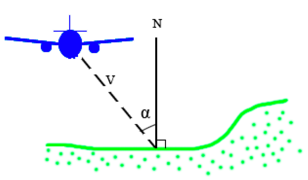
Figure 1. Definition of the incidence angle as the angle between the scan direction and vertical relative to a plane tangent to the local illuminated surface.

Figure 1. Definition of the incidence angle as the angle between the scan direction and vertical relative to a plane tangent to the local illuminated surface.

$$\alpha ={\cos }^{-1}\frac{V\cdot N^{-1}}{\left|V\right|\left|N^{-1}\right|}$$

(6)

2.3. Geometric Waveform Features

The echo width is a quantitative indicator that can evaluate the extent of pulse broadening. When peak detection is employed, the estimated width is at full-width-half-maximum (FWHM) of the pulse; when the Gaussian function is fitted to waveforms, the estimated parameter representing echo width is the standard deviation (S_p,i) of the Gaussian distribution. If necessary, a constant factor of 2.3548 can be applied to convert from S_p,i to FWHM (Equation (7)) [25].

$$FWHM=2\sqrt{2\ln 2}{s}_{p.i}\approx 2.3548s_{p.i}$$

(7)

Several studies of small-footprint waveforms have observed that the echo width of vegetation points is generally greater than that of terrain points [26]. Forest terrain also tends to exhibit larger echo widths than buildings [27]. This implies that the echo width W can be an additional method for discriminating between ground/building returns and vegetation. However, it may be noisy in terms of point-based width information [12]. The results of the factorial experiment performed by Lin et al. [13] suggest the application of echo width information within a pre-defined neighborhood. When dealing with various flight missions, a normalization process must be performed on the echo width. In this study, a normalization process is proposed. First, the coefficient of variation of the echo widths W_cv in the neighborhood (i.e., the nearest 8 points, as defined in the previous section) is estimated, as indicated by Equation (8). It is related to the ratio of the standard deviation STD(W) to the mean Mean(W). W_cv is not significantly influenced by the flight altitude in a statistical sense [13]. This feature is based on contextual information. Second, the concept of Fuzzy Small membership [28] is applied to W_cv.

$$W_{cv}=100\times \frac{STD(W)}{Mean(W)}$$

(8)

Fuzzy logic applies a membership function to express degrees of truth or certainty within the range of zero to one. The standard Fuzzy Small membership function, which is presented in Equation (9) [28], is useful when smaller input values have a higher membership (i.e., they are closer to 1). The function is defined by a user-specified midpoint f₂ with a defined spread f₁. The midpoint has a fuzzy membership of 0.5. The larger spread results in a steeper distribution around the midpoint. Equation (9) was altered to yield Equation (10) to indicate how the transformation is implemented. Through the fuzzy transformation process, W_cv is readily mapped to a scale of 0 to 1; the mapped value is denoted by FW_cv. The midpoint f₂ of the Fuzzy Small membership is defined by the 95th percentile of the W_cv extracted from the lowest points in the large grid cells. The spread-out parameter f₁ has a default value of 5. The lowest points can be readily acquired using the Classify_Ground tool of the TerraSolid^® TerraScan software package. The distances to the nearest Triangulated Irregular Network (TIN) facets and angles to the vertices of the triangle are set to be small values (i.e., an iteration angle of 2 degrees and iteration distance of 4 m). Once the lowest points within the areas of interest are found, the 95th percentile of the corresponding W_cv attributes is estimated.

$$\mu (x)=\frac{1}{1+{\left(\frac{x}{f_2}\right)}^{f_1}}$$

(9)

$$F{W}_{cv}(W_{cv})=\frac{1}{1+{\left(\frac{W_{cv}}{W_{cv}^L({95}^{th})}\right)}^5}$$

(10)

An increase in echo width indicates a range variation within the footprint. When the range variation is low, such as for flat surfaces (e.g., asphalt and mowed grass), the width measurement should be close to that of the transmitted pulse [7]. In areas of rough surfaces, the distributions are wider and the measurements deviate from that of the transmitted pulse. Therefore, the echo width measurements W_cv after transformation indicate the degree of smoothness of the illuminated surface. A greater value for FW_cv indicates a higher probability of being a smooth surface.

In addition to FW_cv, which is a waveform-based roughness indicator, two height-based roughness attributes (RSS_h and dZ) are investigated for feature importance in a classification procedure. The residual sum of squares of the 3D plane fitting (RSS_h) within the 8 nearest points for an individual point of interest is estimated to define the surface roughness. If most of the neighboring points lie on a plane, this value should be very close to zero. This feature is considered a meso-level roughness feature. Additionally, the normalized height dZ is the height difference between the point of interest and the terrain model, which is composed of classified ground points using TerraScan software.

2.4. Classification Strategy

Two supervised classification algorithms, the DT and NN classifiers, are implemented for point cloud classification using Polyanalyst^®. Polyanalyst is a user-friendly data mining system that helps decision support. DTs are a type of fast and popular classification algorithm that enables exploration of the data and easy interpretation of the model. The model resembles a tree with branches, including a number of splits and nodes. In comparison with DT algorithms, NN algorithms may be more robust than statistical classification methods, but they act as a black box. The two classifiers are used to investigate the classification accuracy when using normalized features rather than raw features.

3. Datasets

This study utilizes data from a Riegl LMS-Q680i full-waveform laser scanner, the specifications for which can be found in Riegl [29]. A wavelength of 1550 nm is used. The laser beam divergence angle (β) is 0.5 mrad. The scan angle can be up to ±30°. To obtain a large dynamic range for recording the signal magnitude, the low and the high receiver channels can each be used to record waveforms with an 8-bit quantization level. Sample digital number (DN) values from each channel range from 0 to 255. The low channel is a sensitive channel. The high channel is less sensitive but provides a larger dynamic range, which can accommodate higher amplitude. When the amplitude exceeds a threshold value set by the system, waveform data can be recorded by both channels. To estimate geometric and physical waveform features, the amplitude, echo width, and range for a point of interest must be acquired. The commercial Riegl RiAnalyze software package can export these observations using Gaussian decomposition. The echo width from the Riegl software package corresponds to the FWHM of the pulse, with a unit of 0.1 ns. However, the amplitudes provided are those linearized by Riegl amplitude correction using “LinearizeArray” and “DelogArray” for low and high channel waveforms, respectively [30]. The two arrays are used to estimate the linearized values, which depend on the raw amplitudes.

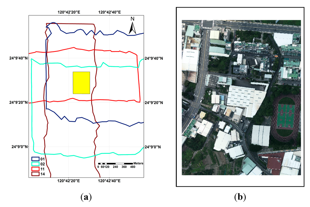
Figure 2. (a) Coverage of four overlapping strips over a homogeneous area. (b) Orthoimage of the study site.

Figure 2. (a) Coverage of four overlapping strips over a homogeneous area. (b) Orthoimage of the study site.

The full-waveform data were collected from a campaign with two different altitudes, both in Taichung city, Taiwan in July 2011. The data were captured at altitudes of approximately 1090 m and 615 m, with a mean point density of greater than 2.5 and 5.5 measurements per square meter, respectively. The study site was a homogeneous area covered by four overlapping flightlines. As illustrated in Figure 2a, the yellow block is the study site (235 m × 306 m), which was selected to investigate the variety of different scan geometries and landforms. Strips 01 and 02 were collected from the same flight mission at an average flight altitude of 1090 m. Strips 11 and 14 were flown across each other on the same flight mission, with an average flight altitude of 615 m. Figure 2b is an orthoimage of the study site

4. Results

4.1. Variety of Raw Waveform Features

Because the amplitude provided by Riegl RiAnalyze is linearized, the range of the amplitude is not from 0 to 255 DN. Values >500 (which approximately corresponds to the starting point of the nonlinear range) could be found in the dataset, in particular at extremely bright surfaces from missions with lower flight altitudes (i.e., strips 11 and 14). Table 1 presents the number of amplitude values per strip. Because extremely high values are not compatible with the linear behavior of raw amplitudes, the backscatter coefficient derived may be problematic. Therefore, samples with linearized amplitudes greater than the 98th percentile of No. 11 are not considered for further quantitative analysis.

Table 1. Number of amplitude values by percent for the four strips in the study site.

Strip	0~500 DN	500~1000 DN	>1000 DN
01	99.95%	0.03%	0.01%
02	99.99%	0.00%	0.00%
11	95.52%	3.22%	1.25%
14	95.83%	4.06%	0.10%

Table 1. Number of amplitude values by percent for the four strips in the study site.

Strip	0~500 DN	500~1000 DN	>1000 DN
01	99.95%	0.03%	0.01%
02	99.99%	0.00%	0.00%
11	95.52%	3.22%	1.25%
14	95.83%	4.06%	0.10%

Figure 3 shows the amplitude point cloud of four overlapping strips. It is evident that amplitudes from different flying heights are quite inconsistent. The effect of the incidence angle on the amplitude can be observed in some roof areas. The yellow highlighted area in Figure 3 represents planes from the same material; however, discrepancies between strip 01 and strip 02 are apparent. Figure 4 shows the width point cloud of four overlapping strips. It is found that less of a discrepancy exists in the width images than in the amplitude images. The width values from rough areas are generally large, whereas those from smooth areas are small. However, it seems that the widths are slightly larger where strong amplitudes are present. For example, white markings on asphalt roads or extremely bright rooftops were acquired in strips 11 and 14 (see Figure 4). As shown in Figure 5, a scatter plot of the linearized amplitude vs. width for the rooftop area (i.e., the red highlighted square in Figure 4) indicates that the width increases with increasing amplitude values. Therefore, caution must be used when exploiting linearized amplitude information. Furthermore, in strips 11 and 14, the width seems capable of separating buildings and roads. The widths of the buildings are slightly greater than those of asphalt but less than those of vegetation. The amplitude seems to affect the echo width at low altitudes (i.e., at the average altitude of 615 m in this study).

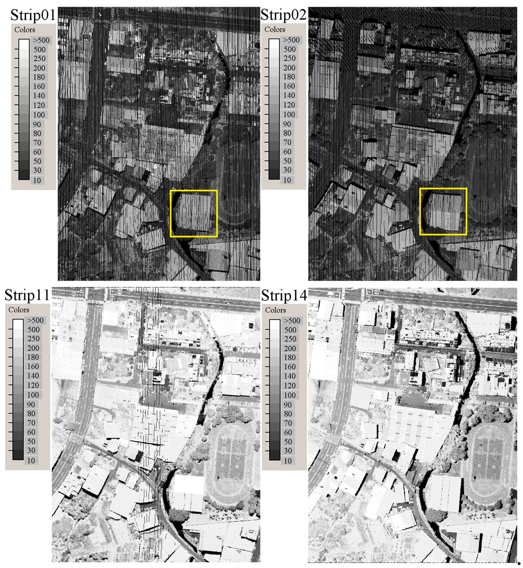
Figure 3. Amplitude point cloud for four overlapping strips. The area inside the yellow box shows where there are discrepancies due to the incidence angle.

Figure 3. Amplitude point cloud for four overlapping strips. The area inside the yellow box shows where there are discrepancies due to the incidence angle.

Figure 4. Width point cloud for four overlapping strips. The white markings on the road inside the yellow box and the roof inside the red box indicate that widths are slightly greater where strong amplitudes are present.

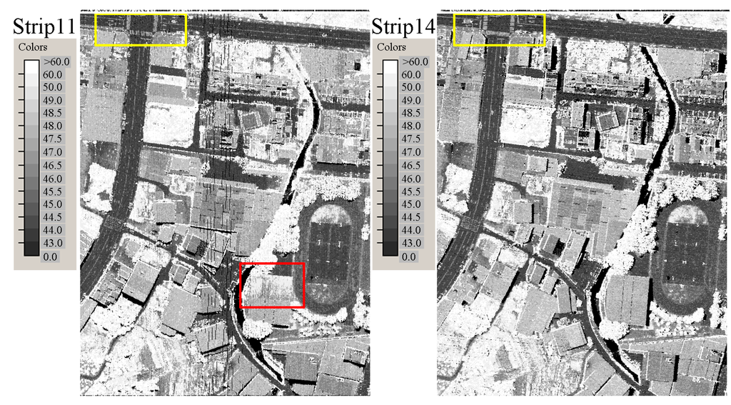
Figure 4. Width point cloud for four overlapping strips. The white markings on the road inside the yellow box and the roof inside the red box indicate that widths are slightly greater where strong amplitudes are present.

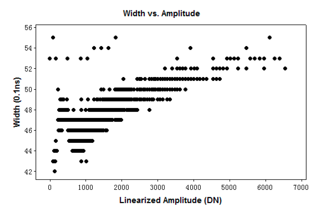
Figure 5. Scatter plot of width versus linearized amplitude for rooftop surfaces with extremely high amplitudes. The samples are taken from the area inside the red box in Figure 4.

Figure 5. Scatter plot of width versus linearized amplitude for rooftop surfaces with extremely high amplitudes. The samples are taken from the area inside the red box in Figure 4.

4.2. Variety of Normalized Waveform Features

4.2.1. Comparison of the Calibration Constant

Because the different incidence angles must be considered before using the amplitude and width, one uses Equation (4) in Section 2.2 to calculate the calibration constant. Assuming a reflectance of 0.25 for asphalt, an individual calibration constant per scan strip is calculated based on the samples from six sections of asphalt road with various scan angles. There are 1345, 1409, 2607, and 3797 total road samples for strips 01, 02, 11, and 14, respectively. A comparison of the mean calibration constant for the strips is shown in Figure 6. It is evident that the mean calibration constants from the same flying mission are similar, but those from different flying missions are substantially different. The calibration constant for each strip is used for the calculation of the backscatter coefficient.

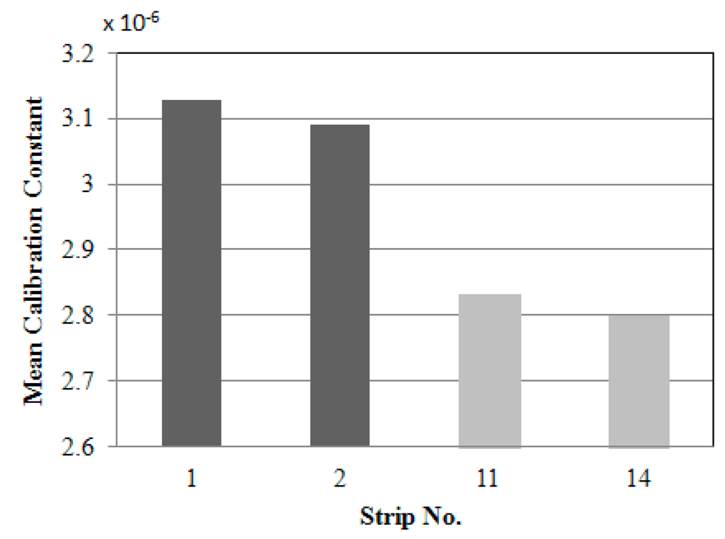
Figure 6. Comparison of calibration constants.

Figure 6. Comparison of calibration constants.

4.2.2. Comparison of the Normalized Features over Various Land Cover Types and Flight Missions

To analyze the difference before and after feature normalization, samples of various land cover types acquired from different flight missions in a homogeneous area were investigated. Figure 7 shows an interval plot of the linearized amplitude, backscatter coefficient γ, width W, and normalized width FW_cv over the six land cover types (i.e., asphalt, cement ground, low vegetation, roof, soil ground and tree canopy). Each interval plot displays the mean and 95% confidence interval. Such plots are especially helpful for comparing groups. It was found that the amplitudes (Figure 7a) are significantly affected by the flight altitude, as expected. The normalized echo feature, which is the backscatter coefficient (Figure 7b), could result in considerable reduction of variation over different flight missions. The normalized width is associated with the degree of surface smoothness. The values of the normalized width (Figure 7d) over low vegetation and canopy are less than 0.5, whereas the values of the normalized width over asphalt, cement ground, soil ground, and roofs are greater than 0.5.

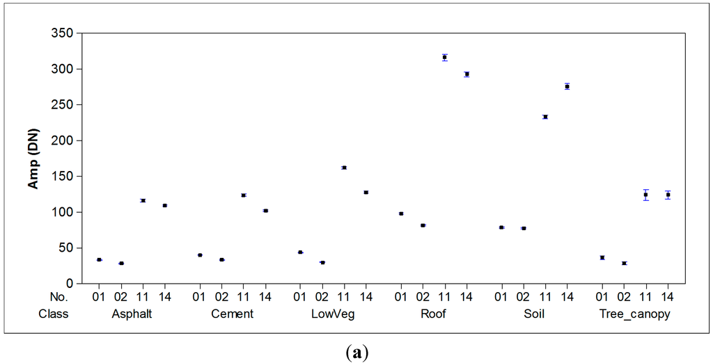
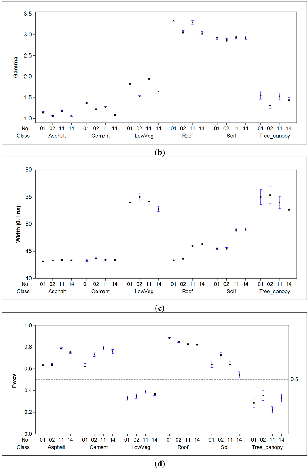
Figure 7. Interval plots of the (a) linearized amplitude, (b) backscatter coefficient, (c) width, and (d) normalized width.

Figure 7. Interval plots of the (a) linearized amplitude, (b) backscatter coefficient, (c) width, and (d) normalized width.

4.3. Effect of Different Feature Combinations on Classification Accuracy

To investigate the effect the on classification accuracy of point clouds acquired from the same or different flight missions with and without normalized features, the overall accuracy of seven types of feature combinations using DT and NN algorithms were analyzed. A data subset of individual flight strip was used for both training and testing in the classification process. The numbers of samples are listed in Table 2. Land cover types of interest are ground, roof, low vegetation, and tree canopy, as shown in Figure 8. These four types were selected because of the feature separation results (see Section 4.2.2). Differences among asphalt, cement ground, and soil ground were not evident. Therefore, those three types were grouped together as one type, which is referred to as ground.

Furthermore, the seven combinations investigated are primarily based on raw waveform features (A{Linearized Amplitude, Width}, B{Linearized Amplitude, Width, and dZ}, and C{Linearized Amplitude, Width, RSS_h and dZ}), normalized waveform features (D{γ and FW_cv}, E{γ, FW_cv, and dZ}, and F{γ, FW_cv, RSS_h, and dZ}), or all possible features investigated in this study (G{Linearized Amplitude, Width, γ, FW_cv, RSS_h, and dZ}).

Table 2. Number of samples over the four strips.

Strip No.	Ground	Low Vegetation	Roof	Tree Canopy
1	1738	666	3521	162
2	1789	553	2602	157
11	2165	1217	3610	226
14	2141	1066	2731	256

Table 2. Number of samples over the four strips.

Strip No.	Ground	Low Vegetation	Roof	Tree Canopy
1	1738	666	3521	162
2	1789	553	2602	157
11	2165	1217	3610	226
14	2141	1066	2731	256

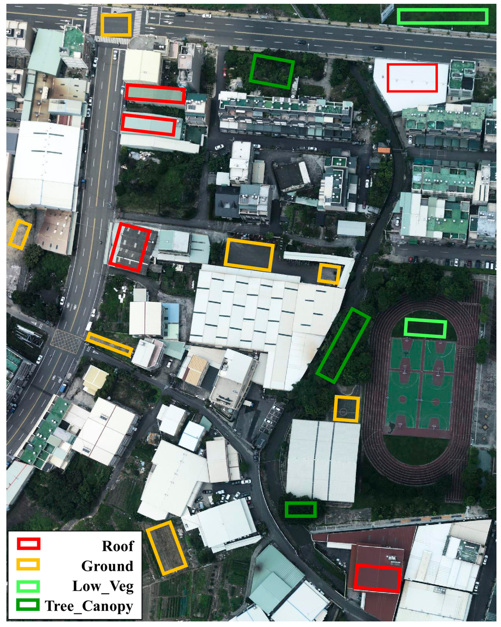
Figure 8. Distribution of samples for four land cover types.

Figure 8. Distribution of samples for four land cover types.

Figure 9 shows the overall accuracy when the training and testing samples originated from the same mission. Among the seven feature combinations investigated, the overall accuracies of combinations B, C, E, and F are relatively high (>95%), while those of combinations A and D are relatively low. The combination G mostly performs well; however, the result of the combination of different strips from the same missions (i.e., 01 and 02 or 11 and 14) may be not as consistent as results from the combination of the same strip and mission (i.e., 01 and 01; 02 and 02; 11 and 11; or 14 and 14). Additionally, the results indicate that such accuracy reduction is not related to the classifiers. However, combinations A and D, which comprise only two features, perform worse. The accuracy of combination A, which comprises raw features, seems slightly better. Nevertheless, in terms of consistency, combinations with normalized features perform better.

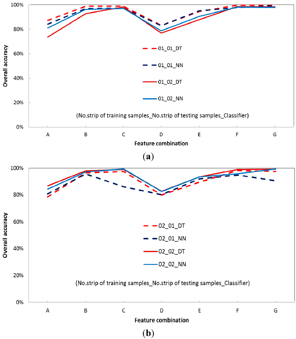
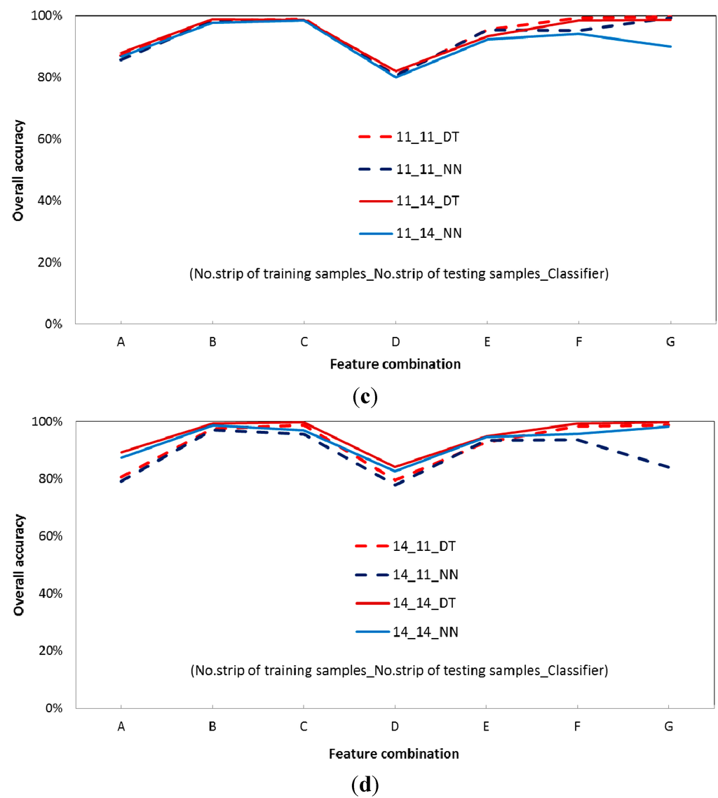
Figure 9. Overall accuracy of feature combinations from data from the same flight missions using the decision tree (DT) and neural network (NN) algorithms: (a) training samples (01), testing samples (01 or 02); (b) training samples (02), testing samples (01 or 02); (c) training samples (11), testing samples (11 or 14); (d) training samples (14), testing samples (11 or 14). Labels on the x-axes are as follows. A:{Linearized Amplitude, and Width}, B:{Linearized Amplitude, Width, and dZ}, C:{Linearized Amplitude, Width, RSS_h, and dZ}, D:{γ and FW_cv}, E:{γ, FW_cv, and dZ}, F:{γ, FW_cv, RSS_h, and dZ}, and G:{Linearized Amplitude, Width, γ, FW_cv, RSS_h, and dZ}.

Figure 9. Overall accuracy of feature combinations from data from the same flight missions using the decision tree (DT) and neural network (NN) algorithms: (a) training samples (01), testing samples (01 or 02); (b) training samples (02), testing samples (01 or 02); (c) training samples (11), testing samples (11 or 14); (d) training samples (14), testing samples (11 or 14). Labels on the x-axes are as follows. A:{Linearized Amplitude, and Width}, B:{Linearized Amplitude, Width, and dZ}, C:{Linearized Amplitude, Width, RSS_h, and dZ}, D:{γ and FW_cv}, E:{γ, FW_cv, and dZ}, F:{γ, FW_cv, RSS_h, and dZ}, and G:{Linearized Amplitude, Width, γ, FW_cv, RSS_h, and dZ}.

Figure 10 shows the overall accuracy for training and testing samples from different missions. Among the seven feature combinations investigated, the overall accuracy of combination F {γ, FW_cv, RSS_h, and dZ} is relatively good and consistent when different flight missions and classifiers were used. An overall accuracy of >93% is possible. In terms of different classifiers applied (i.e., DT and NN), the mean value of the difference in overall accuracy is only 3.08%. It is evident that combinations with normalized features added (i.e., combination D, E, and F) ensure consistency in the overall accuracy. This result is encouraging and indicates that combinations that include normalized features and height-based features are transferable over different flight missions and classifiers. Conversely, the accuracy of the feature combinations with raw features added can be problematic and inconsistent. Furthermore, the combination of all possible features, including raw features, normalized features, and height-based features, performs less well. It is evident that such a combination confuses the DT and NN algorithms. In addition, height-based features (i.e., dZ and RSS_h) play a significant role in the classification procedure. For example, the accuracy of B is generally better than that of A. The accuracy of E{γ, FW_cv, and dZ} is, on average, >12.6% greater than that of D{γ and FW_cv}. The accuracy of F{γ, FW_cv, RSS_h, and dZ} is, on average, 4.6% greater than that of E{γ, FW_cv, and dZ}.

Figure 10. Overall accuracy of feature combination in terms of data from different flight missions using the decision tree (DT) and neural network (NN) classifiers: (a) training samples (01), testing samples (11 or 14). (b) Training samples (02), testing samples (11 or 14). (c) Training samples (11), testing samples (01 or 02). (d) Training samples (14), testing samples (01 or 02). Labels on the x-axes are as follows. A:{Linearized Amplitude, and Width}, B: {Linearized Amplitude, Width, and dZ}, C:{Linearized Amplitude, Width, RSS_h, and dZ}, D:{γ and FW_cv}, E:{γ, FW_cv, and dZ}, F:{γ, FW_cv, RSS_h, and dZ}, G:{Linearized Amplitude, Width, γ, FW_cv, RSS_h, and dZ}.

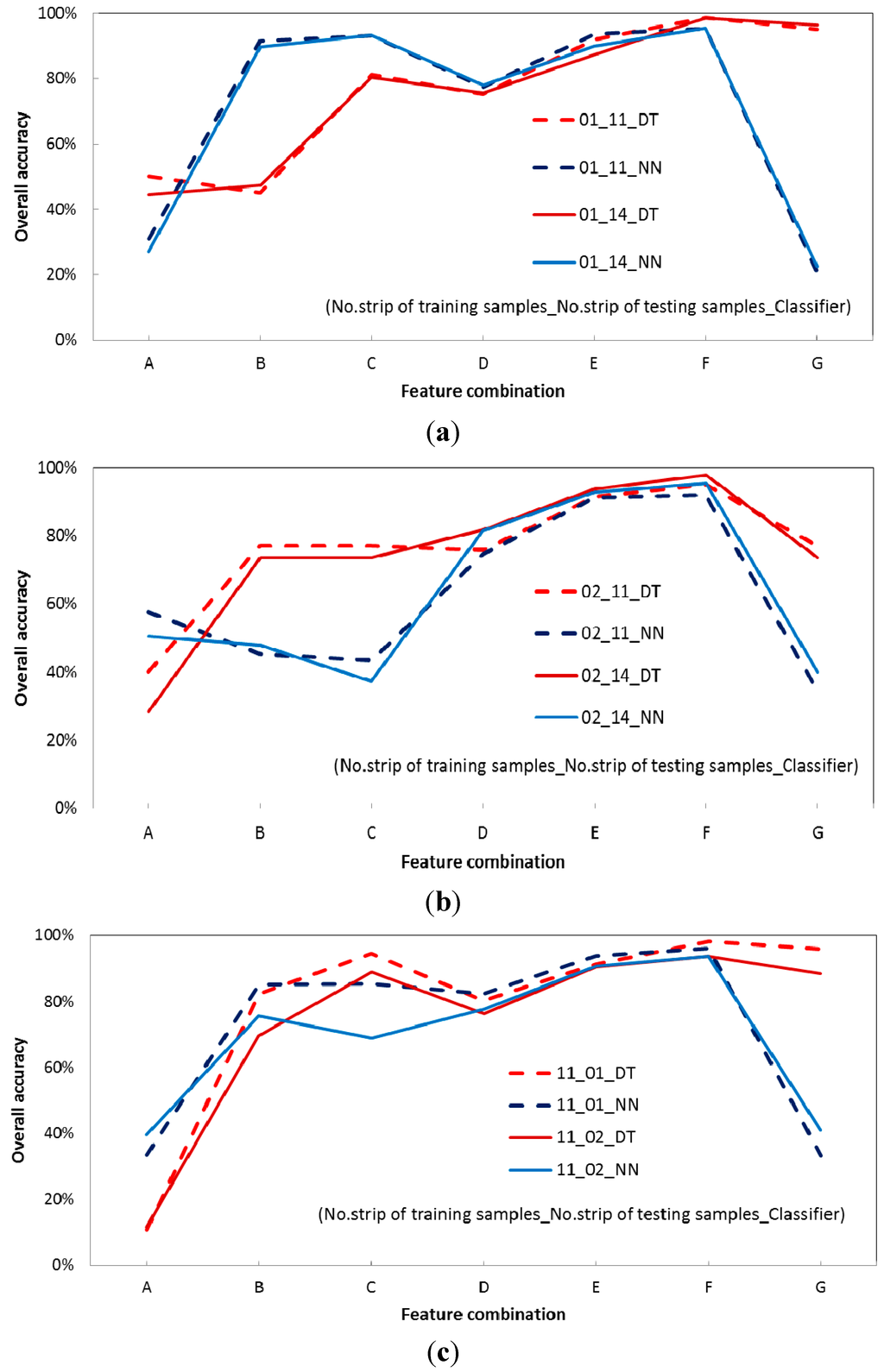
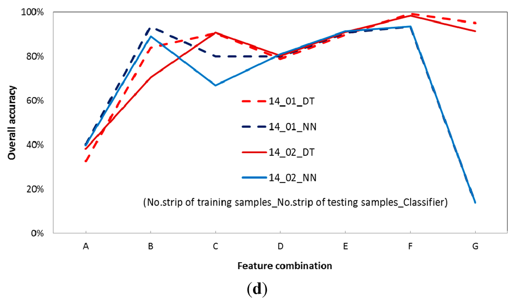
Figure 10. Overall accuracy of feature combination in terms of data from different flight missions using the decision tree (DT) and neural network (NN) classifiers: (a) training samples (01), testing samples (11 or 14). (b) Training samples (02), testing samples (11 or 14). (c) Training samples (11), testing samples (01 or 02). (d) Training samples (14), testing samples (01 or 02). Labels on the x-axes are as follows. A:{Linearized Amplitude, and Width}, B: {Linearized Amplitude, Width, and dZ}, C:{Linearized Amplitude, Width, RSS_h, and dZ}, D:{γ and FW_cv}, E:{γ, FW_cv, and dZ}, F:{γ, FW_cv, RSS_h, and dZ}, G:{Linearized Amplitude, Width, γ, FW_cv, RSS_h, and dZ}.

5. Discussion

The raw waveform features, which are linearized amplitude and width provided by Riegl RiAnalyze, are both found to vary with various flight missions investigated in this study. Furthermore, the linearized amplitude seems to affect the echo width at low altitudes (i.e., strips 11 and 14). It is interesting that such findings are not evident in the datasets with high altitudes (i.e., strip 01 and 02). The width behavior for strips 01 and 02 is consistent with the results of most previously published studies. On the other hand, compared to the amplitude, the backscatter coefficient results in considerable reduction of variation over different flight missions. The backscatter coefficient can be considered to be an absolute physical echo feature when comparing datasets from different missions. Compared to the raw echo width, the normalized width can serve as an index for the degree of surface smoothness.

This study demonstrates how much non-normalized features may degrade the results of classification. The seven combinations are based on raw waveform features ({Linearized Amplitude, Width}, {Linearized Amplitude, Width, and dZ}, and {Linearized Amplitude, Width, RSS_h and dZ}), normalized waveform features ({γ and FW_cv}, {γ, FW_cv, and dZ}, and {γ, FW_cv, RSS_h, and dZ}), or all possible features investigated in this study ({Linearized Amplitude, Width, γ, FW_cv, RSS_h, and dZ}). The result indicates that when the training and testing samples originated from the same mission, the number of the features seems to play an important role. The combination of all possible features {Linearized Amplitude, Width, γ, FW_cv, RSS_h, and dZ}, including raw features, normalized features, and height-based features mostly performs well. However, when the training samples and testing samples are from different flight missions, such combination yields inconsistent results. When treating data from different flight missions, the classifier can be severely affected by inappropriate feature combinations. Selection of a suitable feature combination seems to be more important than selection of a good classifier. In addition, when only the raw waveform features are exploited, users must be cautious about feature transferability between different flight strips. Alternatively, additional height-based features (i.e., dZ and RSS_h) can improve the overall accuracy and consistency.

6. Conclusions

This paper presents an approach to normalize echo features derived from ALS full-waveform data. Normalized features over various land cover types and flight missions are investigated. The effect of different feature combinations on the classification accuracy is analyzed. It is demonstrated that feature combinations based on normalized features and height-based attributes achieve the best and the most consistent results among the seven combinations investigated. An overall accuracy of >93% for the land types of ground, roof, low vegetation and tree canopy was found in data from the same or different flight missions or various classifiers (i.e., the DT and NN classifiers used in this study). However, adding redundant or unnecessary features, whose behavior could vary with flight mission, is not helpful for improving the classification results. Although a robust classifier could be employed, this is not guaranteed to generate acceptable results. Some confusion may occur in the classification. It is suggested that selecting representative features that would not vary with flight missions is more important than considering the robustness of the classifiers employed. It was found that features after normalization proposed in this study can be favorably applied to data from different ALS surveys. In addition, the proposed normalized width can represent the degree of surface smoothness for micro-level structures. The value ranges from 0 to 1. Higher values (closer to 1) indicate smooth surfaces, whereas lower values (closer to 0) indicate rough surfaces. Because the estimate of the normalized width is based on the widths in a pre-defined neighborhood, further research could investigate whether any further improvement is achieved when the neighborhood is defined by object-based segments of physical feature imagery.

References

- Sithole, G.; Vosselman, G. Experimental comparison of filter algorithms for bare-Earth extraction from airborne laser scanning point clouds. ISPRS J. Photogram. Remote Sens. 2004, 59, 85–101. [Google Scholar] [CrossRef]
- Korzeniowskaa, K.; Pfeiferb, N.; Mandlburgerb, G.; Lugmayr, A. Experimental evaluation of ALS point cloud ground extraction tools over different terrain slope and land-cover types. Int. J. Remote Sens. 2014, 35, 4673–4697. [Google Scholar] [CrossRef]
- Song, J.-H.; Han, S.-H.; Yu, K.; Kim, Y.-I. Assessing the possibility of land-cover classification using lidar intensity data. In Proceedings of International Archives of the Photogrammetry, Remote Sensing and Spatial Information Sciences, Graz, Austria, 9–13 September 2002; pp. 259–262.
- Baltsavias, E.P. A comparison between photogrammetry and laser scanning. ISPRS J. Photogram. Remote Sens. 1999, 54, 83–94. [Google Scholar] [CrossRef]
- Höfle, B.; Pfeifer, N. Correction of laser scanning intensity data: Data and model-driven approaches. ISPRS J. Photogram. Remote Sens. 2007, 62, 415–433. [Google Scholar] [CrossRef]
- Alexander, C.; Tansey, K.; Kaduka, J.; Holland, D.; Tate, N.J. Backscatter coefficient as an attribute for the classification of full-waveform airborne laser scanning data in urban areas. ISPRS J. Photogram. Remote Sens. 2010, 65, 423–432. [Google Scholar] [CrossRef]
- Lin, Y.-C.; Mills, J.P. Factors influencing pulse width of small footprint, full waveform airborne laser scanning data. Photogram. Eng. Remote Sens. 2010, 76, 49–59. [Google Scholar] [CrossRef]
- Höfle, B.; Hollaus, M.; Hagenauer, J. Urban vegetation detection using radiometrically calibrated small-footprint full-waveform airborne LiDAR data. ISPRS J. Photogram. Remote Sens. 2012, 67, 134–147. [Google Scholar] [CrossRef]
- Jutzi, B.; Gross, H. Investigations on surface reflection models for intensity normalization in airborne laser scanning (ALS) data. Photogram. Eng. Remote Sens. 2010, 76, 1051–1060. [Google Scholar] [CrossRef]
- Abed, F.M.; Mills, J.P.; Miller, P.E. Echo amplitude normalization of full-waveform airborne laser scanning data based on robust incidence angle estimation. IEEE Trans. Geosci. Remote Sens. 2012, 50, 2910–2918. [Google Scholar] [CrossRef]
- Rutzinger, M.; Höfle, B.; Hollaus, M.; Pfeifer, N. Object-based point cloud analysis of full-waveform airborne laser scanning data for urban vegetation classification. Sensors 2008, 8, 4505–4528. [Google Scholar] [CrossRef]
- Guo, L.; Chehata, N.; Mallet, C.; Boukir, S. Relevance of airborne lidar and multispectral image data for urban scene classification using Random Forests. ISPRS J. Photogram. Remote Sens. 2011, 66, 56–66. [Google Scholar] [CrossRef]
- Lin, Y.-C.; Lin, C.-L.; Tsai, M.-D.; Yu, C.-Y. Influence of varying landforms and flight geometry on echo attributes of full-waveform airborne laser scanning data. In Proceedings of the 34th Asian Conference on Remote Sensing 2013, Bali, Indonesia, 20–24 October 2013; pp. SC01 81–88.
- Hofton, M.A.; Minster, J.B.; Blair, J.B. Decomposition of laser altimeter waveforms. IEEE Trans. Geosci. Remote Sens. 2000, 38, 1989–1996. [Google Scholar] [CrossRef]
- Jutzi, B.; Stilla, U. Measuring and processing the waveform of laser pulses. Opt. 3-D Meas. Tech. VII 2005, 1, 194–203. [Google Scholar]
- Wagner, W.; Ullrich, A.; Ducic, V.; Melzer, T.; Studnicka, N. Gaussian decomposition and calibration of a novel small-footprint full-waveform digitising airborne laser scanner. ISPRS J. Photogram. Remote Sens. 2006, 60, 100–112. [Google Scholar] [CrossRef]
- Jelalian, A. Laser Radar Systems; Artech House: Boston, London, 1992. [Google Scholar]
- Ducic, V.; Hollaus, M.; Ullrich, A.; Wagner, W.; Melzer, T. 3D vegetation mapping and classification using full-waveform laser scanning. In Proceedings of The Workshop on 3D Remote Sensing in Forestry, Vienna, Austria, 14th–15th February 2006; pp. 211–217.
- Lehner, H.; Briese, C. Radiometric calibration of full-waveform airborne laser scanning data based on natural surfaces. In Proceedings of International Archives of Photogrammetry, Remote Sensing and Spatial Information Sciences, Vienna, Austria, 5–7 July 2010; pp. 360–365.
- Briese, C.; Pfennigbauer, M.; Lehnera, H.; Ullrich, A.; Wagner, W.; Pfeifer, N. Radiometric calibration of multi-wavelength airborne laser scanning data. Int. Arch. Photogram. Remote Sens. Spat. Inf. Sci. 2012, I-7, 335–340. [Google Scholar]
- Wagner, W. Radiometric calibration of small-footprint airborne laser scanner measurements: Basic phyiscal concepts. ISPRS J. Photogram. Remote Sens. 2010, 65, 505–513. [Google Scholar] [CrossRef]
- Roncat, A.; Lehner, H.; Briese, C. Laser pulse variations and their influence on radiometric calibration of full-waveform laser scanner data. In Proceedings of ISPRS Workshop Laser Scanning 2011, Calgary, AB, Canada, 29 August–1 September 2011.
- Jolliffe, I.T. Principal Component Analysis; Springer: New York, NY, USA, 2002; p. 487. [Google Scholar]
- Otepka, J.; Ghuffar, S.; Waldhause, C.; Hochreiter, R.; Pfeifer, N. Georeferenced point clouds: A survey of features and point cloud management. ISPRS Int. J. Geo-Inf. 2013, 2, 1038–1065. [Google Scholar] [CrossRef]
- Weisstein, E.W. Gaussian Function. Available online: http://mathworld.wolfram.com/GaussianFunction.html (accessed on 1 March 2015).
- Wagner, W.; Hollaus, M.; Briese, C.; Ducic, V. 3D vegetation mapping using small-footprint full-waveform airborne laser scanners. Int. J. Remote Sens. 2008, 29, 1433–1452. [Google Scholar] [CrossRef]
- Stilla, U.; Jutzi, B. Waveform analysis of small-footprint pulsed laser systems. In Topographic Laser Ranging and Scanning: Principles and Processing; Shan, J., Toth, C.K., Eds.; Taylor & Francis Group: London, UK, 2009; pp. 215–234. [Google Scholar]
- Esri ArcGIS Resources. Available online: http://resources.arcgis.com/en/help/main/10.1/index.html#//009z000000rz000000 (accessed on 7 November 2014).
- Riegl Datasheet LMS-Q680i. Available online: http://www.riegl.com/uploads/tx_pxpriegldownloads/10_DataSheet_LMS-Q680i_28–09–2012.pdf (accessed on 6 June 2012).
- Jalobeanu, A. The full-waveform lidar RIEGL LMS-Q680i: From reverse Engineering to sensor modeling. In Proceedings of ASPRS 2012 Annual Conference, Sacramento, CA, USA, 19–23 March 2012.
© 2015 by the authors; licensee MDPI, Basel, Switzerland. This article is an open access article distributed under the terms and conditions of the Creative Commons Attribution license (http://creativecommons.org/licenses/by/4.0/).