
Applying Terrestrial Laser Scanning for Soil Surface Roughness Assessment


Abstract
: Terrestrial laser scanning can provide high-resolution, two-dimensional sampling of soil surface roughness. While previous studies demonstrated the usefulness of these roughness measurements in geophysical applications, questions about the number of required scans and their resolution were not investigated thoroughly. Here, we suggest a method to generate digital elevation models, while preserving the surface’s stochastic properties at high frequencies and additionally providing an estimate of their spatial resolution. We also study the impact of the number and positions of scans on roughness indices’ estimates. An experiment over a smooth and isotropic soil plot accompanies the analysis, where scanning results are compared to results from active triangulation. The roughness measurement conditions for ideal sampling are revisited and updated for diffraction-limited sampling valid for close-range laser scanning over smooth and isotropic soil roughness. Our results show that terrestrial laser scanning can be readily used for roughness assessment on scales larger than 5 cm, while for smaller scales, special processing is required to mitigate the effect of the laser beam footprint. Interestingly, classical roughness parametrization (correlation length, root mean square height (RMSh)) was not sensitive to these effects. Furthermore, comparing the classical roughness parametrization between one- and four-scan setups shows that the one-scan data can replace the four-scan setup with a relative loss of accuracy below 1% for ranges up to 3 m and incidence angles no larger than 50°, while two opposite scans can replace it over the whole plot. The incidence angle limit for the spectral slope is even stronger and is 40°. These findings are valid for scanning over smooth and isotropic soil roughness.1. Introduction
Terrestrial laser scanners (TLSs) are designed to capture precise and detailed geometric information about natural and artificial objects. These instruments utilize the light detection and ranging (LiDAR) technique to collect point clouds with spatial resolution ranging from several millimeters up to several centimeters, depending on the object distance from the scanner [1]. Besides the geometry information (range, horizontal and vertical angles), some TLSs are able to register backscattered laser intensity, which then can be used to deduce the radiometric properties of the scanned objects [2].
Thanks to the above characteristics, terrestrial laser scanning has been successfully applied to many environmental applications, like forestry, hydrology and geomorphology. For example, tree stems and heights, canopy openness, 3D tree structure, as well as its change detection are just some of the forest-mapping aspects that have been addressed by the TLS data [3–6]. In hydrology and geomorphology, the TLS data have been used, e.g., to characterize the surface of gravel-bed river banks [7–9] or even submerged gravel beds [10], then to quantify depositional and erosional processes in dynamic and complex fluvial systems [11,12] or to classify complex morphological settings, as well as to monitor the landslide displacement [13,14]. Compared to these studies, the application of the TLS data for surface roughness assessment is, however, more challenging, since the surface features that should be described appear already at the millimeter scale, which is about the resolution limit of the contemporary TLSs [1]. Thus, special care should be taken during TLS data acquisition and processing to successfully describe these fine-scale roughness elements.
Surface roughness is a physical property of natural surfaces and also a parameter in many geophysical models. Since each physical process interacts with the specific group of surface features and under the specific range of scales, there is a high diversity in understanding, characterizing and even in naming the surface roughness among the corresponding disciplines. Some of the commonly-used terms are: hydraulic roughness, soil roughness, surface microtopography, snow surface roughness, aerodynamic roughness, etc. [15–20]. Soil roughness, for example, affects infiltration and runoff during a rain event, controls wind erosion and fluid flow and also influences the backscattered energy of radar signals [21,22]. Local surface features, like tillage structure, soil aggregates and particles, are considered to be directly related to the soil roughness, and in the corresponding roughness studies, they are typically described through their regional stochastic properties [23]. Hollaus et al. [24] distinguished between two different types of roughness, the surface and the terrain roughness, where the latter one describes objects that are 20 cm or more above the surface. Most of the soil roughness studies are concentrated exclusively on surface roughness, where it is additionally distinguished between a so-called “oriented” and a random roughness geometry [16,18,23]. In this paper, assessment of the surface roughness associated with a bare soil plot with a random (isotropic) geometry will be analyzed.
There are several methods for soil roughness assessments that involve: (1) different soil height sampling techniques; and (2) different data analysis strategies. Traditional roughness sampling techniques are pin and mesh-board profilers, which collect individual soil roughness profiles with a length ranging from 0.5 m to 4 m and a regular sampling distance ranging from 5 mm to 10 mm along the profile direction [25,26]. A non-destructive alternative for the above roughness measurements are laser profilers. An example of this category is a laser profiler constructed by CESBIO (The Center for the Study of the Biosphere from Space) and ESA (European Space Agency), which is able to sample heights regularly at every 5 mm and collect up to 25 m-long profiles [27]. On the other hand, there is a number of studies where digital images and the stereo-photogrammetric techniques are applied to provide a two-dimensional sampling of soil heights (e.g., [18,28,29]). These data are used to generate regularly-structured digital elevation models (DEMs), which then serve as a base for the roughness analysis. The recent studies of Marzan et al. [16] and Bretar et al. [30] showed, for example, that DEMs with a millimeter grid size can be readily reconstructed with stereo-photogrammetry for plots of 6 m2 to 12 m2. Terrestrial laser scanning is another technique capable of providing precise two-dimensional sampling of soil heights at a similar scale [20,31,32]. In the TLS studies of Barneveld et al. [33], as well as Nield et al. [34], the soil surface was analyzed even over a larger area (up to 120 m2 and 144 m2, respectively), but this was at the cost of the DEM’s resolution, i.e. the DEM’s grid size was much coarser there (1 cm). On the other hand, in the study of Haubrock et al. [35], a 1 mm DEM of micro-erosion plots over ∼1 m2 was generated from data collected by an optical triangulating laser scanner. While all of the mentioned TLS studies apply multiple scanning to mitigate occlusions and improve the spatial resolution of the TLS data, the number of required scans and the resolution that will ensure a certain accuracy level of a roughness index were not investigated.
The sampled soil heights are used to analyze the stochastic properties of soil roughness. This can be done either: (1) in the spatial domain, e.g., by calculating the autocorrelation function [18,36] or variogram [16,17]; or (2) in the frequency domain, i.e., using the roughness spectrum, which is the power spectrum of the sampled soil heights [22,37]. The latter is especially favorable for large datasets, but this approach also involves the discrete Fourier transform (DFT) for which an additional data aggregation into a regularly-structured DEM should be performed. Since the TLS sampling is irregular in the Euclidean space, the original TLS data should be first interpolated into a DEM and then analyzed by the DFT. This interpolation is usually accompanied with smoothing, which is most severe at high surface frequencies, where the most important roughness content is placed. Thus, optimally, the resulting DEM should preserve the stochastic properties of the original surface, as well as the spatial resolution of the original data. However, in roughness studies, the resolution of the used DEMs is usually determined only based on the point density or sometimes even arbitrarily and then reported by the DEM’s grid size. This, however, cannot be applied on close-range TLS data, where the sampling is diffraction limited, and as shown by Lichti and Jamtsho [1], the resolution is a function of both the sampling interval and the laser beam footprint. Thus, such inappropriately-generated DEMs can lead to an inaccurate assessment of soil roughness. Besides, there are several theoretical studies that already showed that some roughness indices, like the correlation length and the root mean square height, are sensitive to data resolution [38–40].
This paper presents the findings of an experiment where a TLS was applied to measure soil surface roughness on a plot with an isotropic, random geometry. Since the stochastic properties of bare isotropic soil surfaces were intensively studied in the past ([23,25,27,36,41], etc.), the focus of this paper is rather on the application of the terrestrial laser scanning for the assessment of soil surface roughness. Particularly, the paper suggests a method for generating a DEM that ensures that the surface’s stochastic properties are preserved at high frequencies and provides additionally an estimate of the DEM’s spatial resolution. Then, it is studied how the number and positions of scans, as well as the DEM resolution affects spatial correlation, the roughness spectrum and four selected roughness indices (correlation length, root mean square height (RMSh), power coefficient and spectral slope). Additionally, a small sub-plot is surveyed with an optical triangulating scanner (OTS), and then, the corresponding TLS and OTS roughness estimates are compared over this area.
The paper is organized as follows: Section 2 explains how the roughness plot was prepared and surveyed and how the laser scanning data were processed. Section 3 starts with presenting the main characteristics of the collected data and continues with reporting the results of this study. Then, in Section 4, the major findings from the Results section are discussed and compared with other studies. Furthermore, this section comments on the suitability of TLS for soil roughness assessment. Finally, conclusions are drawn in Section 5.
2. Materials and Methods
An out-door experiment was conducted to test the potential of terrestrial laser scanning for the soil roughness description. The experiment involved the preparation, measurement and analysis of a bare soil roughness plot.
2.1. Roughness Preparation
An isotropic roughness pattern was prepared on a 2.6 m × 3 m rectangular plot placed in the Botanical Garden of the University of Vienna, in late October, 2013. The plot was generally used as a seed bed for plant reserve growth and was composed of a bare loamy-sand soil, which was rich in organic materials and rather dark in color. The soil is part of the Danube river basin and, generally speaking, contains a notably large portion of sand compared to clay, which is present just in a small amount. The high presence of the organic matter is a consequence of more than 30 years of cultivation. Such an organic-rich soil generally has low reflectance at laser wavelengths compared to other soil types. This negatively affects the strength of the backscattered laser signal, as well as the signal-to-noise ratio, decreasing the quality of the resulting TLS measurements. Thus, the selected soil imposes rather unfavorable conditions for TLS scanning compared to other soil types.
To ensure an isotropic geometry within the plot, the soil was first prepared by a rotary cultivator and then flattened out with a rake. The resulting roughness was mainly driven by randomly-oriented and spatially-distributed soil particles and aggregates, most of them with a size of ∼0.5 cm to 7 cm in diameter (Figure 1b,c). Additionally, some traces of the rake pulling process were present in some parts of the plot. However, their magnitude and amount were too small to disturb the general isotropic and random nature of the plot. Finally, other roughness elements, like small gravel (up to 2 cm in diameter), as well as needles and leaves from the surrounding trees were also present in the plot, though all of them in a very small quantity (Figure 1c).
2.2. Measurement Setup and Acquired Data
The roughness plot was measured immediately upon its formation. The measurements were performed with the Z + F IMAGER® 5006i, an amplitude-modulated continuous-wave (AM-CW) terrestrial laser scanner (TLS) that uses the phase comparison ranging technique. The instrument has a specified precision of 0.4 mm (relevant for targets with a reflectivity of 100%) and a small beam divergence (0.22 mrad), with a beam diameter at the exit of 3 mm [42]. The scanner also has a large vertical field of view (FoV) that starts at 75° below the horizon and which allows its positioning closer to the object. In addition to the TLS measurements, a subplot of ∼0.3 m × 1.2 m was scanned by an optical triangulating laser scanner (OTS), Konica Minolta VIVID® 910i. This scanner provides data with a specified precision of 32 μm for the wide-lens scanning setup, which is one order of magnitude better than the specified precision of the TLS. On the other hand, the typical ground sampling distance (GSD) of this instrument is less than 1 mm, which is far below the TLS’s footprint in a close-range setup (up to 4 mm). Therefore, these data were considered as a reference and used for the validation of the roughness parameters derived from the TLS.
The measurement setup of the TLS is shown in Figure 1a. The measurements started on 23 October 2013 at 13:00 CET and finished approximately one hour later. The weather was mainly cloudy, but also with some short sunny intervals and without wind and rain. The plot was surveyed with 4 scan positions, each placed approximately halfway on the plot’s edges and as close to the plot as the TLS’s vertical FoV allows. The scanner was mounted on a standard wooden tripod adjusted at the maximum possible height (∼1.8 m), which ensures the stability during the scanning. The scanning itself was performed in the “low noise” and “high power” mode, while the sampling resolution was set to “super high”, i.e., 20,000 measurements within the full vertical and horizontal circle [42]. Such a scanning mode requires 17 min per scan position to scan the complete FoV. In addition to this setting, 4 spherical targets (made of Styropor® and each with a radius of 10 cm) were installed at the 4 plot’s edges. These targets were later used as tie points for the relative orientation of the 4 measured TLS scans. A similar setting was already applied successfully for a vegetation survey with the same TLS instrument [5]. During the complete surveying time, it was ensured that these targets were static and visible from each scan position.
The measurement setup of the OTS was slightly atypical. Since this is primarily an indoor instrument that has a relatively small FoV compared to the TLS, a special construction was installed over the subarea to survey a strip with several overlapping OTS scans. Unfortunately, a picture of this particular setup was not available, and thus, Figure 1d shows the identical setup over another roughness plot, which is not considered in this paper. As can be seen there, the construction acted as a platform made of two adjustable metal trestles, which were used to support a horizontally-positioned aluminum ladder. The OTS scanner was mounted on the ladder and faced down toward the soil at a relative height of ∼0.7 m. Additionally, the construction was covered by special ultra-light, first-aid blankets to introduce the indoor lightning conditions, which is required for successful scanning with the OTS. The surveying was then done by a successive ladder sliding and capturing individual OTS scans. The scans were acquired using the wide lens with a focal distance of 8 mm, which, for our setup, provided a rectangular object coverage of ∼0.4 m × 0.3 m and a ground pixel size of ∼0.7 mm. Alternatively, “tele” and “middle” lenses could have been used, as well. However, the increase in precision and resolution that they bring is minor and at the cost of the FoV, which would only increase the number of individual scans.
In total, 10 individual OTS scans were collected in the form of a strip and in the direction approximately parallel and close to one of the plot’s edges. It was ensured that the successive scans had at least a 70% overlap along the larger edge of the OTS’s FoV, which also determined the final strip length (∼1.2 m). The strip width, on the other hand, was driven by the smaller edge of the OTS’s FoV (∼0.3 m at the ground). To resolve an initial co-registration between the OTS and TLS data, two small wooden spherical targets (3 cm in radius) were placed at the beginning and end of the OTS strip. They were firmly fixed to the ground by 20 centimeter-long screws and were visible in both OTS and TLS data. Later, in the preprocessing phase, these parts were excluded from the OTS data, which, together with slightly inclined strip directions to the plot’s sides, restricted the effective area to 0.18 m × 1 m for the OTS strips.
2.3. Data Processing
TLS data were processed through two main steps. The first step aimed at extracting valid measurements (points) from the raw TLS data, while in the second step, these valid points for each of the 4 TLS scans were transformed into a common coordinate system. During the transformation, the soil heights were also detrended, which is the prerequisite for almost any roughness analysis [22,23]. This section explains each of these two main tasks in more detail.
2.3.1. Pre-Processing
The pre-processing of the raw point clouds was done in the “Z + F Laser Control” software, similarly to the pre-processing done in [4]. Several predefined filters were applied to remove (1) irrelevant measurements, (2) low-quality measurements and (3) erroneous measurements, which are associated with the AM-CW ranging technique. First, points outside the plot area, i.e., irrelevant points, were discarded by applying a simple polygon filter. Then, points with a small intensity value were removed from the data by an intensity filter with the default settings. These points have a low signal-to-noise ratio, and thus, they are generally considered as low-quality measurements [43]. Finally, points that are so-called mixed pixels were removed automatically by applying the mixed-pixel filter and single-pixel filter implemented in the software. These points are associated with an erroneous range value that appears when an AM-CW ranging system samples a target that has individual scatterers distributed along different ranges within the laser beam [43]. In soil roughness scanning, such cases appear, e.g., when the laser beam illuminates simultaneously both the top of a large soil aggregate (first individual scatterer) and the underling soil surface (second individual scatterer).
Depending on the reflectance, illuminated area and relative distance between the individual scatterers, the resulting range may appear anywhere along the laser’s line of sight, i.e., in front, behind or between the soil aggregate’s top and the soil in the background. In all three cases, mixed-pixel points provide the false geometry of soil aggregates, while in the latter case, they cover the occluded area, providing also a false impression about the coverage and point density of the TLS data. Thus, the mixed pixels have to be removed before any data quality and roughness analysis. Figure 2 shows automatically detected mixed pixels (yellow points) in one of our TLS scans, applying the default settings suggested by the software. Although this filter setting performed the best in our case, i.e., up to a 5-m range, it was also observed that the filters’ performance became questionable for larger ranges. Thus, automatic filtering of the mixed pixels may be an issue in the case of larger roughens plots.
2.3.2. Data Transformation and Detrending
Each TLS or OTS scan is acquired in its own local coordinate system, which will be named here the sensor’s own coordinate system (SOCS). To analyze the two datasets jointly, all of the individual scans were transformed from their SOCSs into one common coordinate system, named here the object coordinate system (OCS). The transformation was done through three consecutive steps. First, the relative orientation was resolved independently among the TLS scans and among the OTS scans. This resulted in two point-cloud blocks, one from the TLS scans and another from the OTS scans, where each of them was built in its own block coordinate system (BCS). Then, in the second step, the OTS block was co-registered globally to the TLS block. Finally, the co-registered scans were all transformed together from the TLS’s BCS to the OCS.
A coarse, relative orientation of the TLS scans was done using the 4 spherical targets installed at the plot’s corners. These targets were measured semi-automatically in each TLS scan, and then, their centers were used as tie points to derive the transformation parameters (three rotation angles and three translation increments) for each TLS scan. This was done within an adjustment procedure implemented in the Z + F Laser Control software, where the scan taken from Position 1 (Scan 1) was fixed. This ensured that the resulting TLS block had a coordinate system identical to the SOCS of Scan 1. The average deviation between the corresponding tie points after the adjustment was 4.8 mm. Then, an additional fine relative orientation of the TLS scans was done using an in-house implementation of the iterative closest point (ICP) algorithm. As a result, the average 3ddistance between the corresponding points among each TLS scan pair ranged from 0.9 mm to 1.1 mm. The relative orientation of the OTS scans was also done by the same ICP algorithm, where one of the OTS scans was kept fixed. The average distance between the corresponding OTS points after the relative orientation was 0.1 mm.
The co-registration of the OTS to the TLS block was done through an initial co-registration followed by a fine co-registration. The initial co-registration was done using the 4 small spherical targets installed at the OTS strip’s corners. The spheres’ centers, derived independently from the OTS and TLS block, were used as tie points in an adjustment that provided the 6 global parameters for the rigid body transformation between the two blocks. These parameters were then applied to transform each OTS scan into the TLS’s BCS. Finally, a fine registration was performed with the mentioned ICP algorithm in which all of the TLS and OTS scans were co-registered autonomously to one another. The average 3D distance between all of the corresponding TLS and OTS points was 1.2 mm after applying the ICP.
Since roughness analysis should be performed on detrended heights, the co-registered scans were once more transformed into final OCS, where soil roughness heights were free from a global planar trend. This transformation was done by defining the z-axis of the OCS as parallel to the normal of an orthogonal-distance regression plane that was fit through all of the TLS points within the plot. The center of gravity of these points was taken to be the origin of the OCS, while the direction of one plot’s side (defined with two large spheres) was taken as the x-axis of the OCS. This means that the z-coordinate of the measured points in the OCS represents the linearly detrended component of soil roughness heights. In practice, when large plots are considered (e.g., plot sides of 25 m or larger), the global trend may also appear to be different from planar, e.g., a higher order polynomial surface [36], and in this case, data should be accordingly detrended to arrive at roughness heights. The second and third order polynomial surfaces were also estimated for our plot, and their root mean square (RMS) of the fit errors were 11 mm and 10 mm, respectively, whereas for the linear fit, the RMS error was also 11 mm. Since the RMS errors are practically identical, the linear model was selected, because it is the simplest one and also in accordance with most of the roughness studies ([23,40,41], etc.).
2.4. Roughness Analysis
Soil roughness was analyzed in both the spatial and frequency domain. To enable the conversion between the domains, gap-free digital elevation models (DEMs) were built, and discrete Fourier transform (DFT) was used. The roughness analysis itself was then performed on profiles, which were actually rows or columns of the generated DEMs. The focus of the analysis was on understanding the nature of spatial correlation associated with the profile heights, as well as on deriving the conventional roughness parametrization, i.e., root mean square height (s) and correlation length (l).
2.4.1. DEM Generation
Gap-free DEMs offer the regular structure of soil heights, which is the required data format for an application of the DFT. Thus, two different interpolation methods were consecutively applied to compute the interpolation at every grid node. First, the moving plane method was performed, providing an interpolation that is derived from the local regression plane estimated on all of the points within a circular neighborhood. The moving plane interpolation was selected, because the locally-inclined plane is a much more appropriate model for the soil surface compared to, e.g., the local horizontal plane, which is the case for the mean and median interpolators. Besides, the later interpolators also tend to provide step-like DEMs, which might additionally hamper the roughness assessment. The neighboring points used for the interpolation were the linearly-detrended measurements of soil heights given in the OCS, while the radius of the circular neighborhood is the data aggregation parameter, which controls the amount of smoothing, i.e., the resolution, of the interpolated DEM. Multiple radius sizes were applied to understand their influence on the soil roughness assessment and to select accordingly the optimal one for the DEM generation. The local regression plane was not possible to estimate for some grid nodes, because either there were not enough neighboring points (more than 3) or the neighboring points were too inclined (nearly vertical), providing a singular covariance matrix. For these grid nodes, the interpolation was computed from the corresponding triangular facets of a triangular irregular network (TIN) built on the grid nodes, which were interpolated by the moving plane interpolation in the previous step. Such an interpolation strategy was applied on different subsets of measurements, e.g., on single TLS’s scan, or two or four merged TLS’s scans, providing the corresponding 1-mm gap-free DEMs, used in the subsequent analysis.
2.4.2. Roughness Description
The interpolated profile heights (the DEM’s rows or columns) are treated here as realizations of an isotropic, zero-mean process with a Gaussian probability distribution function. This is a conventional and widely-used roughness model [25,36,41], which, considering the plot size and that the roughness geometry was prepared, also appeared to be a reasonable assumption for our analysis. This model is completely described once the autocorrelation function (ACF) of the profile heights is known. This means that an empirical ACF should be first estimated, and then, the root mean square (RMS) height and the correlation length parameters should be determined from the applied ACF model.
In this paper, the empirical ACF was estimated in the same way as in [25,41], i.e., as the Fourier transform of the power spectral density (the roughness spectrum) obtained as the periodogram. This is equivalent to:
2.4.3. Soil Spatial Correlation and Measurement Noise
The soil heights that are used in this study contain also random measurement errors. These errors are treated here as a stochastically-independent and spatially-uncorrelated additive component, i.e., white noise. As such, the measurement noise may negatively affect the signal-to-noise ratio at high frequencies, and many soil roughness elements that should be described are actually present in this frequency region. Then, the assumed measurement noise has an ACF that approaches the delta function in the ideal case. Thus, the empirical ACF estimated from a noisy soil profile will be only biased at the zero lag , while the ACF estimates at other lags will just become more uncertain than without the measurement noise. This means that the measurement noise just introduces more power into the roughness spectrum, resulting in an overestimation of the s parameter. For the correlation length, this means that the decorrelation by e−1 (∼37%) in the empirical ACF happens at a smaller lag compared to the profile without the noise, resulting in an underestimation of the l parameter. Following simple geometry, the amount of this underestimation will depend on the magnitude of the measurement noise, as well as on the local slope of the empirical ACF function around the . Thus, the measurement noise simply biases the classical roughness parametrizations s and l, which was the reason for considering additional roughness parametrization in the analysis.
Two extra parameters were additionally included: one to observe the nature of the soil spatial correlation at small lags and another parameter to observe the nature of the soil roughness spectrum at high frequencies. The former parameter is the power coefficient p of the power-model ACF function that allows a better description of spatial correlations, which are neither exponential nor Gaussian [44]. The power model of the normalized ACF is given by:
The second parameter is the so-called spectral slope α, which is the slope of a regression line used to model the roughness spectrum given in the logarithmic scale [37]. This means that the power spectral density S(f), i.e., the roughness spectrum, of a surface should behave in the linear-scale frequency domain as:
3. Results and Analysis
3.1. Characteristics of the TLS Data
Table 1 reports the most important statistics of the acquired TLS point clouds within the plot. Values given in the range column represent the distance from the origin of the TLS’s coordinate system to the scanned objects within the plot. Point density, sampling interval and laser footprint diameter are reported for the furthest and the nearest 20-cm bands of the plot with respect to the corresponding scan position.
These values are given within the columns named “near” and “far”, respectively. The reported point density (Dband) is the median value of the number of TLS points per cm2 (pts/cm2) within the corresponding zone. The sampling interval (Δband) was then estimated from this point density by assuming a uniform point distribution within 1 cm2, i.e., where band stands either for the near or the far plot zone. The laser footprint diameter was calculated based on the non-linear expansion equation for the short ranges [46] and using minimum and maximum ranges for the near and far plot zones, respectively. Finally, the last column reports the ratio of the laser footprint diameter to the sampling interval. This value indicates the TLS sampling mode, and for values larger than one, the laser footprints of the adjacent rays were overlapping one another during the scanning, introducing the so-called correlated sampling [1]. As can be seen from Table 1, all of the TLS scans were acquired in the correlated sampling mode.
For merged scan data, the range and footprint statistics from Table 1 remain similar, while the median point density in the near and far plot zones changed to 220 pts/cm2 and 329 pts/cm2 for the merged opposite scan data and all four scans, respectively. The median point density within the whole plot changed from 60 pts/cm2 to 152 pts/cm2 and 322 pts/cm2 for the two opposite scans and all four scans, respectively. Thus, the spatial distribution of the points improved by including the opposite scans, while for all four scans, the densities at the plot edges become almost identical to the global plot density. All of the merged scan data also have the correlated sampling mode.
Figure 3a shows a scatter plot of the point density and mean range over the plot, both taken from corresponding 1-cm rasters, which were generated using the data of Scan 3. The high variability of the point density at short ranges (the near plot zone) is driven by the local incidence angle and a notably higher median point density compared to the far plot zone (Table 1). It can be also seen that the TLS’s point density drops exponentially from the near to far plot zone. This was also confirmed by the remaining three TLS’s scans, which are shown in Figure 3b. Figure 3c shows a cumulative void area over the range. The void area represents the proportion of cells that does not contain any TLS measurement in a 2-mm raster built over the whole plot. The cell size of 2 mm was selected to match approximately the sampling interval in the far plot zone (Δfar). In this way, the void area values actually indicate the portion of the plot that was bridged by the TIN interpolation in the respective gap-free DEMs. As can be seen from Figure 3c, this happens between 20% to 35% of the plot area for the DEMs built from the individual TLS scans. It should be mentioned here that the void areas do not contain the footprint centers of the laser beams, but some of the void areas may still be covered by the footprints from the laser rays, the centers of which fall within the adjacent cells.
On the other hand, Soudarissanane et al. [47] showed in their experiment that incidence angles also affect the point density, as well as the signal-to-noise ratio of the measured points. Thus, the above results can be seen from this point of view instead of considering only the range. Figure 3d shows the scatter plot of the range and the incidence angle values for our four single scans. These functions can be used to deduce the incidence angle at which the void area or the point density changes due to a change in range. For example, void areas larger than 5% appear in Scan 3 at ranges larger than 3.2 m and incidence angles larger than 50° (Figure 3c,d). The deduction based on Figure 3d will be used later in the text whenever it is necessary to introduce certain restrictions on both the range and incidence angle. It should be noted that the incidence angle is here defined as the shortest angle measured in the vertical plane from the local normal to the laser beam vector in the OCS. The local normal was derived from the planar trend of the plot (Section 2.3.2) and was pointing upwards, i.e., in the direction of the z-axis of the OCS. The direction of laser beam vector was set from the measurement point towards the origin of the TLS’s coordinate system.
The range and incidence angle values describe also the relative position of the scanner to the measured object, i.e., the measurement setup [47]. Thus, the clustering of range-incidence-angle functions for Scan 1, Scan 2 and Scan 4 in Figure 3d means that these scans have a similar measurement setup, whereas the range-incidence-angle function of Scan 3 is slightly biased to the right. This then means that Scan 3 performs the same incidence angles as other scans, but at slightly larger ranges, i.e., it has the best measurement setup among the acquired TLS scans. This scan position was actually taken from the edge of the neighboring plot, which is slightly uplifted compared to our plot (the right side in Figure 1a and also the background area in Figure 1c). This gain in the instrument height with respect to the observed plot resulted in the better acquisition geometry of Scan 3, which is clearly reflected in Figure 3d. In the case that the instrument height improves even more (e.g., by increasing the height of the tripod), the range-incidence-angle function would just be biased more to the right and cover smaller incidence angles. An ideal TLS measurement setup would result in a horizontal range-incidence-angle function at, e.g., 20° or a lower incidence angle. However, this is not possible due to the oblique acquisition architecture of the contemporary TLSs. On the other hand, the OTS data used in our experiment would appear as a vertical range-incidence-angle function at approximately a 0.7 m-range and with a length of several degrees starting from the 0° incidence angle.
Figure 4b,c shows how the void area was spatially distributed within the plot for Scan 1 and for the two opposite scans (Scan 1 and Scan 3) merged into one common point cloud (Scans 1&3), respectively. Figure 4b shows that 24.1% of the plot area was interpolated by the TIN method in the gap-free DEM generated from Scan 1. As can be seen there, most of the void area is concentrated in the far plot zone, i.e., at ranges larger than 4 m. Figure 4c shows that when the data from the opposite scan are additionally used, the occlusions are significantly reduced within the plot. The red regions marked by yellow rectangles in Figure 4b,c are places where the small wooden sphere (used in the block co-registration) were installed.
3.2. Overview of DEM Sets
The analysis presented in the paper is based on a series of differently-generated DEMs. These DEM sets differ in the data source used for their generation, e.g., OTS or TLS point clouds, or, further, in the case of the TLS data, in the number of scans used. Then, there are DEM sets generated over different subparts of the plot or even over the whole plot area (see Figure 4a). Furthermore, some DEM sets were generated using different neighborhood sizes for the DEM interpolation. To overcome this complexity, Table 2 gives an overview of all of the DEM sets, organized according to the particular objectives of the performed analysis.
As can be seen from Table 2, the coming sections will follow the mentioned objectives and will use the introduced nomenclature in Table 2. Nevertheless, the DEM sets will be explained in detail within each section; thus, Table 2 should just give a general overview of the performed analysis and the respective datasets.
3.3. Effects of Neighborhood Size on Soil Roughness
DEM Set 1 was used to analyze the effects of the neighborhood size parameter used during the moving plane interpolation step. As can be seen from Table 2, this set contains DEMs generated from all four merged TLS scans and over the rectangular subplot area (0.18 m × 1 m) surveyed with the OTS scanner. The DEMs were interpolated as explained in Section 2.4.1 setting the neighborhood diameter size for each DEM within the set differently. In total, the neighborhood size was set 16 times, taking values from 1 mm up to the 100 mm, while the grid sizes of the 16 resulting DEMs were always set to 1 mm. For the analyzed subplot, this means that each DEM contained 180 rows with 1000 soil heights regularly spaced at 1 mm from one another over the 1-m row length.
3.3.1. Roughness Spectrum
Figure 5a–c shows the shaded heights of three DEMs selected from DEM Set 1. These DEMs were interpolated using the neighborhood diameters of 1 mm, 3 mm and 6 mm, and will be called here 1-mm DEM, 3-mm DEM and 6-mm DEM, respectively. Based on the given shadings, it looks like the 1-mm DEM contains all of the relevant elements of the soil roughness, which are, however, buried in noise. In the 3-mm DEM, this noise is significantly reduced, while the relevant soil roughness elements are still preserved. The latter is, however, not the case for the 6-mm DEM, where small soil aggregates, as well as the noise are not visible any more. The noise dominating in the 1-mm DEM is actually the measurement noise, which is, due to the extremely small neighborhood size, reflected in the DEM’s heights. Generally, the applied moving plane interpolation behaves similarly to the moving average, i.e., as a low-pass filter, and thus, the size of the neighborhood area regulates how much of both measurement noise and roughness features will be smoothed out in the resulting surface.
The smoothing effect driven by the neighborhood size can be better seen in the frequency domain. Figure 5d shows the mean roughness spectra of the three DEMs, which were estimated with the Fourier transform applied on the DEMs’ rows. As was expected, the spectrum of 1-mm DEM (the red curve) has the highest power, thanks to the portion of the measurement noise that is reflected due to the small neighborhood size. The spectrum of the 3-mm DEM (the green curve) performs along all of the frequencies between the spectra from 1-mm and 6-mm DEMs. Since the RMS height is equal to the area below the roughness spectrum [22], the resulting estimates of roughness parameter s will be biased from one another proportionally to the area between their corresponding roughness spectra. Another interesting point is that the roughness spectrum of the 3-mm DEM performs a white noise roll-off at wavelengths smaller than 3 mm (the right dashed vertical line in Figure 5d). This behavior of the roughness spectrum indicates that the applied grid size is probably smaller than the resolution of our data, which then caused such informationless behavior below 3 mm. The same roll-off can also be seen in the spectrum of the 1-mm DEM. There, the spectrum continues to perform an inclination towards the white noise, even over a broader frequency band, which is due to a weak signal-to-noise ratio coming from the small neighborhood size.
The roll-off of the spectrum from the 6-mm DEM has a completely different shape. It starts around 6 mm (which is actually equal to its neighborhood size) and declines slower than the 3-mm DEM’s spectrum in the same frequency band. Furthermore, the variability of the 6-mm DEM’s spectrum is significantly reduced along the roll-off frequencies compared to lower frequencies. The low variability in this frequency band is perfectly in accordance with the use of the interpolation step, since the associated interpolation (a low-pass filter) affects such frequencies more than those far before its cut-off frequency. This suggests that the shape of the 6-mm roughness spectrum may not reflect the inherent soil spatial correlation well at these frequencies. Finally, the deformation of the 6-mm spectrum exists also in the opposite direction, towards low frequencies. However, the shapes of the 3-mm and 6-mm spectra are very similar there, though the latter appears to be more inclined. This will generally introduce bias in the spectral slope when it is estimated within this frequency band. It should be also mentioned that the starting frequency in Figure 5d (log10(f) = −1.6 mm−1) is the place where the relative difference between the 3-mm and 6-mm roughness spectra becomes less than 10%, while the left vertical dashed line marks the frequency where this difference is at the maximum.
The above example showed the importance of the neighborhood size setting when laser scanning data and DEMs are used in soil roughness analysis. Although all of the considered DEMs should represent the same soil roughness, it is apparent from Figure 5 that they will lead to different roughness estimates, as well as different natures of soil spatial correlation at high frequencies. Thus, an optimization is required to arrive at a suitable neighborhood size, which will minimize the impact of the measurement noise and oversmoothing on the roughness spectrum at high frequencies. The determination of such a neighborhood size is discussed in Section 3.4.
3.3.2. Roughness Indices
The impact of the neighborhood diameter size on the roughness indices was analyzed from DEM Set 1. Figure 6a–e shows box plots of the roughness indices ld, lm, s, p and α (Sections 2.4.2 and 2.4.3) estimated from the 16 DEMs of DEM Set 1. Thus, each box-plot compares 16 sets of 180 index’s values estimated from the 180 rows of the corresponding DEMs. In Figure 6a–e, these sets are denoted by the neighborhood size of the corresponding DEM and plotted over the x-axes of the box plots. It should be noted that the selected neighborhood sizes within the TLS series do not have a constant increment, which can be also seen on the x-axes of the box-plots.
Figure 6b shows that the median of the model correlation length lm enlarged from 83.4 mm to 87.9 mm for the 4 mm and 20 mm neighborhoods, respectively, which is an increase larger than 5%. On the other hand, the dispersion in the correlation length decreased by 25% for the same neighborhoods. The mentioned dispersion actually reflects the spatial variability of the correlation length within the subplot, which then means that a DEM with neighborhood sizes of 20 mm or larger does not depict this soil property well any more. The observed changes in the correlation length and its variability happened because small soil aggregates were smoothed out by increasing the neighborhood size, i.e., soil variability is reduced, resulting in the observed: (1) underestimation of the inherent variability of the correlation length; and (2) overestimation of the inherent correlation length. It should be also mentioned that the model correlation length constantly underestimate the direct correlation length, which for the 4-mm DEM was about 8%. This may indicate that the applied ACF model does not perfectly describe soil correlations locally, i.e., at lags similar to the correlation length value.
The RMS height parameter reacted opposite of the correlation length, i.e., constantly decreasing while increasing the neighborhood size. The smoothing of the small soil aggregates caused the 5% relative decrease in both the s value and its dispersion between the 4-mm and 20-mm neighborhoods. This is slightly surprising, since it is generally considered that the correlation length is more difficult to estimate than the RMS height [23,36,39,41]. This, however, does not seem to be the case here, i.e., for the over-smoothing effect caused by non-optimal data aggregation.
Figure 6d shows how the power coefficient p changes when small soil elements are smoothed out. When all of the relevant soil elements are present in the DEM, the soil heights within the subplot shows a tendency towards an exponential spatial correlation. This is generally the case for isotropic soil roughness analyzed at similar scales [25,27,36]. However, as soon as the neighborhood size increases, p starts to converge to a Gaussian spatial correlation. This means that the over-smoothing effect may also lead to misinterpretation of the soil spatial correlation when a large neighborhood size is selected. This can also be seen in Figure 6f, where the number of exponentially-correlated rows per each DEM is reported. This number was calculated by comparing the RMS errors of the Gaussian and exponential autocorrelation fits per each row and counting the number of rows where the RMS error of the exponential fit was smaller. Figure 6f shows that the 4-mm DEM has almost an equal number of exponentially- and Gaussianly-correlated rows. This is also consistent with the p values, the median of which is 1.4, while their dispersion is large enough to allow both correlation models. In other words, there are many profiles with a p value larger than 1.5, which most likely caused the RMS error of the Gaussian fit to be smaller compared to the exponential fit. The DEMs with a smaller neighborhood size have slightly more exponentially correlated rows, which may be due to the measurement noise that is still present in these DEMs. On the other hand, the DEMs with 40-mm or larger neighborhoods do not have any more exponentially-correlated rows, and their p values are 1.8 or larger. Finally, the 5% relative error of parameter p happened already between the 4-mm and 10-mm neighborhoods, which is slightly earlier compared to the previous indices.
The most interesting results, however, come from the spectral slope α (Figure 6e). This roughness index shows a global minimum for the 4-mm DEM and then features almost a constant median for the neighborhoods larger than 20 mm. As was discussed in Section 3.3.1, the measurement noise, as well as the roll-off effects cause the roughness spectrum to be more inclined towards a white spectrum than towards its inherent inclination at high frequencies. Therefore, the DEM where the measurement noise and the roll-off effects are minimized is the one that has the highest inclination of the roughness spectrum. This corresponds to the minimum of the spectral slope (Figure 6e). This offers the possibility for an optimization of the spectral slope with respect to the neighborhood size, which is explored in the next section.
3.4. Neighborhood Size and Spectral Slope
The behavior of the spectral slope around its global minimum is analyzed here in more detail. This was done using DEM Sets 2.1, 2.2, … and 2.6 (Table 2). The first five DEM sets are based on the TLS data, while Set 2.6 is based on the OTS data. Further, the first two TLS sets were built from single TLS scans, i.e., DEM Set 2.1 from Scan 1 and DEM Set 2.2 from Scan 3. Then, DEM Sets 2.3 and 2.4 were built from the point clouds where two opposite TLS scans were merged, i.e., combing Scan 1 and Scan 3 into Scans 1&3, as well as Scan 2 and Scan 4 into Scans 2&4. DEM Set 2.5 was built using all of the TLS points, i.e., the points collected from the four scans.
Figure 7 shows the spectral slope values estimated from the six DEM sets. These sets contain a much larger number of DEMs due to a finer setting of the neighborhood diameter size. For the five TLS sets, this parameter cover values from 1.5 mm to 5.5 mm, and for the OTS set, from 1 mm to 3 mm, but always with the same increment of 0.1 mm. This resulted in 41 and 21 DEMs per each TLS and the OTS series, respectively. The different span in the neighborhood size caused the x-axis of the OTS set (Figure 7f) to have slightly different limits from the x-axes in the TLS sets (Figure 7a–e). The y-axes, however, are identical in all of the figures.
As can be seen from Figure 7, the spectral slope confirmed the global minima (the red circles) for all six sets and under the much more intense neighborhood sizes. It is only the OTS set that seems to be not large enough to materialize the rising side of the minimum well. However, this will not affect the analysis, since the focus is on the global minimum here. The spectral slope values at the global minimum for the DEM sets based on Scan 1, Scans 1&3 and the four scans are consistent with one another, as well as with the OTS set (Figure 7a,d–f). Scans 1&3 and the four scans caused an underestimation in the spectral slope with a relative error of about 5% comparing to the OTS data. Scan 1, on the other hand, caused a slight overestimation (around 1%) of the spectral slope. One of the reasons for the slightingly larger relative error of the estimates based on the merged scans could be the errors that follow the relative orientation of the TLS scans. Another factor could be the unfavorable measurement setup of Scan 3. As can be seen in Table 3, Scan 3 has incidence angles that are not smaller than 60°, while Scan 1 (with the relative error of the spectral slope within 1%) has incidence angles not lager than 40°. Two TLS sets, one based on Scan 3 and another on Scans 2&4, appeared to be inconsistent with the remaining three TLS sets, providing a large bias (15% relative error) in the spectral slope compared to the OTS data. The reasons for such surprising results will be discussed in the next section.
For the five TLS sets, the global minimum happens at the neighborhood sizes between 4 mm and 4.5 mm, while for the OTS set, it happens even earlier, at 2.8 mm. Following the analysis from the two previous sections, these values identify the DEMs where almost all of the relevant soil elements should be present, while most of the measurement noise should already be filtered out. This means that these DEMs contain the most complete and accurate level of detail on the soil roughness among all of the generated DEMs in this study. Additionally, these DEMs minimize the spectral slope, i.e., maximize the fractal dimension, at high frequencies, and therefore, they were selected as the most appropriate for the subsequent analysis.
3.5. Comparison of Soil Roughness Derived from OTS and TLS Data
The comparison of the two datasets was done over the subplot area and based on six DEMs (DEM Set 3 in Table 2), each of them selected from the corresponding DEM Sets 2.1, 2.2, … and 2.6. The selection was done according to the optimal neighborhood sizes determined in Section 3.4. Shaded models of these DEMs are shown in Figure 8. The shading in Figure 8a is based on the OTS data and visually looks like the one that contains the highest level of detail on the soil roughness among the selected DEMs. This was generally expected, since (according to the specifications) this instrument should provide higher resolution data with a smaller measurement noise compared to the TLS scanner. Furthermore, the OTS point cloud covers the subplot continuously, which means that there was no need to bridge the no data regions with the TIN interpolation. This is not the case with the two DEMs based on the single TLS scans (Figure 8e,f).
The unfavorable acquisition geometry (high incidence angles and low point density) of Scan 3 caused the corresponding DEM to have a completely deformed geometry at scales up to the largest soil aggregate (Figure 8f). These two factors are much more favorable in the case of Scan 1, and therefore, the corresponding DEM (Figure 8e) does not contain extremely large occlusions, while the point density is almost enough to ensure the same level of detail as in the OTS DEM.
The DEMs from two opposite scans do not have problems with occlusion any more (Figure 8c,d). However, they perform certain pattern, which seems to “elongate” the soil aggregates’ edges in a particular direction. For the DEM based on Scans 2&4, the elongation of the soil aggregates is along the larger subplot side, which also corresponds to the direction of the laser line of sight within the subplot. For the DEM based on Scans 1&3, this elongation is along the smaller subplot side, which is again the direction of the laser line of sight. The same effect can be also seen in the individual scans. The first explanation for this effect is the interpolation over the shadow area of a scan. A shadow appears along the line of sight. A second possible explanation for this directional pattern may be the nature of the AM-CW ranging technique, i.e., mixed pixels. In the preprocessing step, the mixed pixels were removed, but only for the case when the laser beam illuminates the top of a soil aggregate and the background soil. However, when the laser beam illuminates the bottom of a soil aggregate, as well as the foreground soil, the resulting range is derived from a sum of the two phasors corresponding to each of the two scatterers. This then leads to a range that is slightly shorter than it should be and, eventually, makes the soil aggregates more elongated in the direction of the line of sight. As can be seen in Figure 8b, when a DEM is based on all four scans, this directional pattern is not visible any more. The shadow areas of one scan are typically filled up by points from another scan. This improvement, however, is at the cost of the soil roughness details, which becomes slightly less than in the case of, e.g., the DEM based on Scan 1 (Figure 8e). Especially at edges, points from the poorer acquisition geometry cause this (small) degradation. Two yellow rectangles in Figure 8b,e delineate the area where this loss in roughness is visible in the respective shadings.
The difference observed in the DEMs’ shadings are also analyzed in the frequency domain by comparing the DEMs’ roughness spectra. Figure 9 shows the mean spectra of each TLS DEM after subtracting the mean spectra of the OTS DEM. It was assumed that the OTS DEM depicts the soil roughness in the greatest detail among the six selected DEM, and thus, it was taken as a reference for the comparison. As can be seen from the figure, the relative difference between the OTS power spectrum and almost all TLS spectra does not exceeds 1 dB at wavelengths larger than 50 mm. The 1-dB difference appears slightly earlier and later only for Scan 3 and Scan 1, respectively. The spectrum of Scan 1 has generally the smallest difference for the OTS spectra over the whole frequency domain, which reach their maximum of 4 dB at approximately the 6.5-mm wavelength. This confirms the convincing visual impression of the corresponding shaded model, where the level of soil roughness detail appeared to be almost as rich as in the OTS shading. The spectra based on (1) Scans 1&3 and (2) on the four scans behave similarly to Scan 3, only with a larger maximum difference of 4.8 dB, as well as 6 dB, respectively. On the contrary, the spectra differences of (1) Scan 3 and (2) Scans 2&4 appeared slightly different, indicating that their corresponding DEMs also perform a different spatial geometry. This was already noted in the visual comparison of their shadings in Figure 8.
The question is now how these differences in geometry of the DEMs affect the roughness indices. Part of the answer is already given by Figure 7, where the spectral slope was analyzed. The consistency in the spectral slope among the OTS and the three TLS datasets is most probably the consequence of sampling the profiles perpendicularly to the laser line of sight. This means that even a difference of 4 dB at the 6.5-mm wavelength in the roughness spectrum cannot introduce a change in the spectral slope larger than 1%, as long as the profiles are sampled perpendicularly to the TLS’s directional pattern. However, when the profiles are sampled along the line of sight (the DEM based on Scans 2&4), the spectral slope can be underestimated by 15%. The same amount of underestimation also happens when the scan position is set more apart from the subplot (Scan 3). Such data are accompanied by large occlusions and large incidence angles, which are the main reasons for the observed underestimation.
The response of the remaining three indices on the directional pattern is shown in Figure 10. Again, index values estimated from the individual rows of the six DEMs are presented there with the corresponding box-plots. Additionally, the 5% bounds around the median of the OTS estimates are marked by the dashed horizontal red lines. The medians of s and l turned out not to be so sensitive for the mentioned deformation in DEM geometry, while in the medians of p, the deformations were reflected slightly, but not so clearly as for the spectral slope. This means that as long as the errors in the roughness spectrum are below 1 dB at wavelengths larger than 50 mm, the RMS height and the correlation length cannot change by more than 5%, when they are estimated from 1-m profiles. It should be also mentioned that the observed sensitivity of the parameters α and p may come from the fact that they are estimated from a relatively narrow high-frequency band, which is generally more affected by the DEM deformation, while s and l are estimated from a broader band, where the magnitudes at low frequencies are much larger and, thus, predominantly influence the resulting values.
3.6. TLS Directional Pattern and Profile Sampling
As is shown in the previous section, the directional pattern has only a significant impact at high frequencies and, consequently, on the indices that are estimated from this domain (α and p). Additionally, the results suggested that the sampling across the directional pattern can compensate for the consequent uncertainties in the index’s values. To offer more comprehensive support for the above statements, additional analysis was carried out on three 1-m2 subareas within the plot. Since the roughness estimates are a function of the profile length [25,27,36,39,40], squared areas were selected to allow an easier comparison of the estimates. Figure 11a shows the locations of these subareas, which were selected to be close either to one plot side or to the center of the plot. Per each subarea, three different DEMs were generated always using the 4-mm neighborhood: first, based on all four scans, second based on Scans 1&3 and third based on Scans 2&4 (DEM Set 4 in Table 2). Since the subareas were squares, the roughness spectra, as well as the roughness indices were estimated independently from both DEMs’ rows and columns. This means that the consistency of the index parameters was tested in both directions, along the x-axis (using the DEM’s rows) and along the y-axis (using the DEM’s columns).
Figure 11b shows three mean roughness spectra estimated from the rows of the three corresponding DEMs generated for Subarea 3. Considering the relative scan positions to the plot, this means that the spectrum based on Scans 1&3 (Spectrum 1&3) was estimated from the profiles sampled across the directional pattern, while the spectrum based on Scans 2&4 (Spectrum 2&4) was estimated from the profiles sampled along the directional pattern. The spectrum based on four merged TLS scans (four-scan spectrum) was considered here as the reference, since, according to Section 3.5, the directional pattern is not visible any more in its DEM, while its estimates are still consistent with the OTS estimates. To allow a better interpretation, an additional figure was prepared (Figure 11c), where the four-scan spectrum was subtracted independently from Spectrum 1&3 and Spectrum 2&4. The dotted and full lines are used there to indicate the differences of the spectra estimated along the x- and y-axis, respectively.
As can be seen from Figure 11b,c, all of the spectra are almost identical at wavelengths larger than 50 mm, demonstrating that the directional effects are negligible within this frequency band. However, this is not the case for the frequency band that corresponds to the wavelengths between 50 mm and 10 mm, where Spectrum 1&3 and Spectrum 2&4 departed in opposite directions from the four-scan spectrum. This means that independently of the profile sampling strategy, the spectral slope, as well as the spatial correlation will be highly inconsistent within this frequency band due to the TLS’s directional pattern. The RMS height, on the other hand, will be in the same frequency band, either overestimated or underestimated, depending on weather the profiles are sampled across or along the directional pattern, respectively. The spectrum based on the across profiling, i.e., Spectrum 1&3, continues to overestimate the four-scan spectrum almost constantly along all of the wavelengths smaller than 10 mm, which demonstrates that the two datasets perform the same nature of spatial correlation within this frequency band, while having biased RMS height values from one another. This is not the case for the along profiling, i.e., Spectrum 2&4, which intersects the four-scan spectrum in the same frequency band. The same behavior of the roughness spectra was also observed for the other two subareas (the results are not presented here).
The roughness index values were also estimated for all three subareas and from the same DEMs. Figure 12 reports only the values estimated over Subarea 3, since the other two subareas confirm the same findings. The index values are displayed as box-plots grouped into two sections: the first is named the x-axis section, indicating that the values were estimated from the DEMs’ rows, while the second is named the y-axis section, indicating that the values were estimated from the DEMs’ columns. The box-plots’s names reflect the TLS scans, which were used to generate the DEMs. It should be noted that each box-plot summarizes 1000 index values estimated from 1 m-long profiles.
As can be seen from Figure 12a,b, the box-plots within each section are consistent with one another, regardless of whether the profiles are sampled across or along the directional pattern (Box-plots 1 and 3 and 2 and 4). On the other hand, the index values estimated from the rows (the x-axis section) and then from the columns (the y-axis section) are biased against one another, which reflects the degree of spatial anisotropy within Subarea 3. The consistency of the box-plots within each section for the RMS height and the correlation length confirm the observation from Section 3.5 that these two parameters are not sensitive to the TLS’s directional deformations. The same conclusion can also be drawn for the parameter p based on Figure 12c, where the box-plots are also consistent. Interestingly, for the p parameter, the box-plots for the profiles sampled along the x-axis, as well as along the y-axis are also consistent, which indicates that this parameter does not reflect the spatial anisotropy observed by s and lm. Finally, Figure 12d demonstrates that only the spectral slope parameter is again found to be sensitive to the directional pattern. There, the box-plots related to the along profiling (Box-plots 2 and 4 in the the x-axis section and Box-plots 1 and 3 in the y-axis section) are inconsistent with the other two box-plots by more than 15%. Interestingly, the parameters α and p also showed that the soil is isotropic at high frequencies, which is probably due to a rather round form of soil aggregate, as well as its random spatial distribution within the subarea.
The above analysis demonstrated that the directional pattern has little impact on wavelengths larger than 50 mm. For smaller wavelengths, i.e., with values comparable to the size of the soil roughness elements, this pattern causes an overestimation in the roughness spectrum. This happens at high frequencies, where the roughness magnitudes are generally small. Therefore, this overestimation corresponds to a relative error in the correlation length and in the RMS height under 5%. If, however, the nature of soil spatial correlation up to the 50-mm lag is important to characterize, then either all four TLS’s scans or two opposite scans and profiles sampled across the laser line of sight should be used to estimate the spatial correlation at this scale.
3.7. Comparison of Soil Roughness Derived from Single and Multiple TLS Scans
This section analyzes whether two opposite scans or even a single scan can replace the data from the four merged TLS scans, while preserving a similar accuracy for the s and l parameters. To answerer this, four DEMs were generated over the whole plot (2.6 m × 3 m) using four different scan configurations: (1) single Scan 1; (2) single Scan 3; (3) merged Scan 1 and Scan 3; and (4) all four scans. These DEMs that belong to Set 4 in Table 2, were interpolated using and were interpolated using the 4-mm neighborhood setting, which corresponds to the optimal neighborhood size derived for the four-scan configuration in Section 3.4. This neighborhood was selected because the DEM based on the four-scan configuration was taken here as the reference. The four-scan DEM actually offers the best representation over the whole plot among the alternative DEMs. This is because the OTS data were not available for the whole plot, while the single-scan DEMs are not accurate in the far plot zone (Section 3.5). The two-scan DEMs (Scans 1&3 and Scans 2&4), on the other hand, have a directional pattern (Section 3.6), which was not the case for the selected four-scan DEM.
Figure 13a shows how the profile’s heights taken from a single or two opposite scans are correlated with the heights of the same profile derived from all four scans. The profile’s number is counted in the direction of the plot’s y-axis, which means that profile Number 1 is closer to Scan Position 1, while profile Number 3000 is closer to Scan Position 3 (Figure 4). Since the whole plot was analyzed, this means that the profile length was 2.6 m. Figure 13b,c reports the relative accuracy of the indices s and lm (estimated from single or two opposite scans) with respect to their values estimated from the four scans. The negative relative errors mean underestimation, while the positive values mean overestimation of the index values with respect to the four scans.
Figure 13 shows that the combination of two opposite scans can fully replace the four-scan setting with a relative error in both roughness parameters of less than 1%. Furthermore, the DEM’s heights interpolated from the two opposite scans are almost identical to the DEM’s heights interpolated from the four scans (their correlation is better than 99% for all of the profiles within the plot). The relative errors of the indices estimated from the individual scans have a different behavior when the location of the profile departs from the scan position. Figure 13b,c shows that profiles closer to the scan position (the near field) slightly overestimate the index values derived from the four scans, as well as from the two opposite scans. Then, approximately after half of the plot, they start with the underestimation, which systematically increases till the end of the plot, which is opposite of the scan position. For example, the relative error of the RMSh for Scan 3 and Scan 1 exceeds the 1% limit at profile Numbers 358 and 2705, which happens approximately at scanning ranges larger than 4.2 m and 3.9 m, respectively. For the single scans, the point density gets lower and the incidence angles, as well as the ranges become larger in the far field. As shown in Section 3.5, this even smooths out larger soil aggregates, resulting in the observed underestimation of s. On the other hand, in the near field, the single scans have an optimal acquisition geometry, which allows one to depict slightingly greater level of detail compared to the merged scans, where the points from the poorer acquisition geometry are added. These factors caused the observed overestimation of s in the near field. As expected, completely the opposite happened with the model correlation length. The individual scans first underestimate lm based on the four scans, and then, in the further plot zone, they continue with systematical overestimation. For Scan 1, the 1% overestimation limit of this index happens at profile Number 1703, which corresponds approximately to the range of 3.0 m and an incidence angle of 55° (Figure 13c,d). Interestingly, the relative error of the model correlation length estimated from Scan 3 fluctuates around a 1% limit almost in the whole second part of the plot. A similar behavior of the relative errors and height correlations, which are reported in Figure 13, was also observed when Scan 2, Scan 4, Scans 2&4 and the four scans were analyzed together (these results are, however, not shown here).
4. Discussion
4.1. Optimal Neighborhood Size and the EIFOV
The spatial resolution of the DEMs used in this study should be limited by the the resolution of TLS data used for their interpolation. On the other hand, Section 3.4 showed that although the DEMs’ grid size was set to 1 mm, their spatial resolution was rather driven by the neighborhood size defined during the interpolation. Thus, the question is whether the optimal neighborhood size is consistent with a theoretical resolution measure for TLS point clouds, e.g., with the effective instantaneous field of view (EIFOV) suggested by Lichti and Jamtsho [1].
Figure 14 shows the EIFOV values calculated over the TLS ranges observed within our plot. The values were calculated by imposing the same assumptions on the system modulation transfer function (MTF) as in [1]. The blue curve comes from the theoretical sampling calculated from the horizontal angular increment specified for the “super-high” sampling mode of the Z + F IMAGER® 5006i instrument and assuming a perpendicular laser beam on the object. The latter is, of course, not the case for our measurement setup, and therefore, a corrected EIFOV (green line) was also calculated based on the point density that was directly estimated from individual TLS scans and which was already reported in Figure 3. Additionally, the optimal neighborhood sizes deduced for Scan 1 and Scan 3 (Section 3.4) are plotted at the ranges that correspond to the respective distances of these two scan positions with respect to the subplot. The optimal neighborhood sizes of the merged TLS data are not plotted here, because their neighboring points may have completely different ranges.
As can be seen from Figure 14, the optimal neighborhood sizes overestimate the spatial resolution of the individual TLS point clouds within the plot. This was expected, because the modulation transfer function associated with the applied interpolation method additionally lowers the spatial resolution of the DEMs compared to the point clouds. Another interesting result is that the uncertainty of the corrected EIFOV due to the range is about 2 mm within the plot. Compared to Figure 7 (Section 3.4), this value also corresponds to the uncertainty of the neighborhood size that is associated with the 1% relative error in the optimal spectral slope value. Such a variation in the neighborhood size does not change the relative errors of the s and l by more than 2%, as is shown by Figure 6 in Section 3.3.2. This means that the EIFOV and the optimal neighborhood size are consistent with one another for the applied measurement setting. Thus, the EIFOV value can also be used to determine the optimal neighborhood size under the 5-m TLS ranges. On the other hand, the optimization of the neighborhood size presented in Section 3.4 can then be seen as a practical approach to optimize the spatial resolution of a DEM interpolated from point clouds collected up to the 5-m TLS range.
4.2. Optimal DEM and the Fractal Dimension
The optimization done in Section 3.4 ensures that the resulting DEM minimizes the spectral slope at high frequencies. This roughness index is directly related to the fractal dimension D, which (when estimated from the profiles) is given by [48]: D = (5 − α)/2. Thus, it can be also formulated that the optimization in Section 3.4 maximizes the fractal dimension of the high-frequency roughness elements, while the measurement noise, as well as the loss in roughness detail are minimized. The optimization then leads to DEMs that will have an optimal resolution, as well as a distinctive stochastic property associated with the spatial correlation of the high-frequency roughness elements. The only assumption made to arrive at these optimal DEMs was that the roughness magnitudes should behave similarly to fractals in this frequency band. Thus, it was not assumed that the model given by Equation (4) is valid over the whole frequency domain, but rather within a small band. This is a fair assumption, especially for the soil surfaces, where the roughness is found to be predominantly exponentially correlated [25,36]. For such a spatial correlation, it is already known that its roughness spectrum approaches the fractal model at high frequencies [37]. Nevertheless, the experiment performed in this study certainly cannot answer whether the fractal dimension at high frequencies can be optimized for surfaces that have spatial correlations different from the exponential. A special study that will consider a wide range of surface roughness patterns should be carried out in order to answer this question.
It should be also mentioned that the interpolation strategy applied to ensure the gap-free conditions in the optimal DEM might not be appropriate for all applications. Large soil aggregates imposed occlusions on the TLS line of sight, and the occluded areas were later interpolated using the TIN method, which certainly does not describe the shape of the soil aggregates correctly. However, the results from Section 3.5 showed that these effects do not affect the s and l parameters significantly. Only in the case when the roughness at high frequencies should be described may the interpolation method have a significant impact. As was shown in Section 3.4 for large occlusions (e.g., Scan 3), the spectral slope value can be completely misinterpreted when estimated from the high frequencies. Another case where the interpolation may have a significant impact is the non-correlated sampling, i.e., when the average distance between neighboring points is larger than the laser beam footprint. In such cases, the choice of the interpolator will control the modulation of the roughness spectra much more strongly, and thus, stochastic interpolators, like Kriging, might be more appropriate. Nevertheless, the moving plane interpolation still remains a reasonable choice to model soil roughness within the 4-mm neighborhood from TLS data acquired in the correlated sampling mode.
4.3. Conditions on the Laser Beam Footprint
The results in Section 3.3.2 show how the roughness values react when the spatial resolution of DEMs is reduced by enlarging the neighborhood size. Generally speaking, the same effect may also appear when a series of point clouds with a decreasing spatial resolution are used instead of the series of DEMs interpolated using different neighborhood values. Therefore, the result in Section 3.3.2 can also be seen as a way of simulating how the loss in point cloud resolution influences the index values. This then offers a possibility to introduce the conditions on TLS sampling under certain index’s accuracy, as was done for the case of an ideal sampling in [38,39].
As is shown in Section 3.3.2, both s and l change by more than 5% when the neighborhood size increases from 4 mm to 20 mm. As the neighborhood size is an estimate of the spatial resolution (Figure 14), the above statement can be extrapolated on TLS point clouds. In this case, this would mean that the point cloud of 20-mm or a lower spatial resolution may introduce a relative error in both s and l that is larger than 5%. For the contemporary TLSs, which are rather diffraction- than sampling-limited, this would mean that the laser footprint should be under 20 mm to fulfill the 5% standard in the relative error. Particularly, for the TLS used in this study, such a condition on the laser footprint is fulfilled under a 45-m range. However, such a surprisingly weak condition on the TLS range is only valid in the case of an ideal acquisition geometry, i.e., when the sampling line of sight is perpendicular to the object. Thus, this condition cannot be applied when the standard TLS tripods are used. The reason for allowing such a large laser footprint diameter can be due to the insensitivity of the s and l parameters on the very small roughness components, which was reported within Section 3.3.2. Thus, for roughness studies where the spatial correlation at high frequencies is important, this condition has to be revised according to the parameters that are more sensitive to the changes in this frequency band, e.g., α or p. For such applications, the optimal DEM from Section 3.4 offers the best trade-off between the measurement noise and the roll-off effects. Thus, the applied 5% standard on the relative error actually limits the departure of the considered point cloud from the point cloud that reflects the high frequency roughness the best.
The sampling conditions are usually not instrument oriented, but rather, expressed in terms of the correlation length. For example, Oh and Kay [39] found that the sampling interval should be at least 0.2 of the correlation length to obtain the index values with ±5% precision. For the median correlation length (ld = 118 mm) estimated from all of the rows within the plot, this would mean that the spatial resolution should be ∼50 mm or better. Comparing this to the 5% condition on the laser footprint diameter (20 mm), it appears that the latter is more than two-times stronger, which was generally expected, because of the additional modulation due to the laser beam. In another theoretical study, Ogilvy and Foster [38] found that the sampling interval must be less than one tenth of the correlation length to detect the exponential nature of the spatial correlation around the origin, i.e., at small lags. For our plot, this would mean that the spatial resolution should be ∼12 mm or better to depict the exponential nature of the high-frequency roughness. In our study, the inherent nature of the spatial correlation at high frequents was ensured by the optimization of the fractal dimension in this band, providing the optimal DEMs with a resolution between 4 mm and 4.5 mm, which is almost three-times better than the condition suggested by [38]. Ogilvy and Foster [38] also stated that when the sampling interval is larger than two thirds of the correlation length, the exponentially-correlated roughness may be misinterpreted as a Gaussian. For our experiment, this means that the spatial resolution should be larger than 150 mm to misinterpret the exponentially-correlated rows with a Gaussian. This condition can be best compared with the change in the p parameter and in the number of exponentially-correlated rows, reported in Figure 6d,f, respectively. The latter figure showed that at a spatial resolution around 40 mm or lower, all of the profiles performs the Gaussian spatial correlation, while the 5% relative error in p happens already at the spatial resolution around 10 mm. This is again more than three-times stronger than the condition suggested by [38].
It should be noted that the above condition on the TLS spatial resolution was derived from the correlation length estimated from the 2.6-m profiles of a smooth isotropic soil roughness plot. Such short profiles generally lead to the underestimation of the inherent correlation length of an isotropic soil roughness [25,27,36,39,40]. Thus, the imposed restriction on the TLS resolution is rather valid for roughness studies performed over similar isotropic roughness and at similar scales. To introduce more general conditions, which are independent of, e.g., the plot scale or roughness magnitude, a more extensive analysis should be done.
4.4. Suitability and Limitations of TLS in Soil Roughness
Terrestrial laser scanning was shown to be appropriate for soil roughness analysis according to several aspects. First, TLS offers high-resolution point clouds with low measurement noise at the plot scale. Section 3.4 showed that the spatial resolution of our optimal DEMs is between 4 mm and 4.5 mm, which is, e.g., more than ten times better than the ideal sampling condition imposed by Oh and Kay [39]. The TLS’s resolution is also more than ten-times smaller than the wavelength of the C-band (∼5.7 cm), which is, according to Ulaby et al. [22], sufficient for the application of modeling the backscatter of C- and L-band radar satellites. Then, the average 3D distance between the corresponding points among each TLS scan pair ranged from 0.9 mm to 1.1 mm, which is a good indicator for the TLS’s relative accuracy within the plot. As shown by Lievens et al. [40], these relative accuracies do not have a significant impact on the soil moisture retrieval from the radar backscatter. Another of the TLS’s advantages is that many standard processing tools are already available for processing raw TLS data [49,50]. As was demonstrated in this study, all of the important preprocessing tasks were successfully carried out by applying the standard software settings. Then, TLS is an active remote sensing technique, which allows measurements at any time of the day. Finally, the TLS is portable and needs a maximum of 20 min per station for scanning.
There are also certain limitations that are associated with TLS. The most striking one is certainly the directional pattern, which is a consequence of the AM-CW ranging technique. However, this feature is not only a problem for the AM-CW TLS, but also for other ranging techniques. For example, in the case of pulsed TLS, the measured range results from the decomposition of the transmitted pulse convolved with the surface [51], which again affects the accuracy of the estimated range for the mixed pixels. Then, stereo imaging is also associated with an averaging within the pixel (the aperture diffraction limit) or even over several pixels when the circle of confusion is not optimally set [52]. On the other hand, Sections 3.5 and 3.6 demonstrated that the directional pattern does not affect the roughness spectrum at wavelengths larger than 50 mm, introducing a relative error in the s and l parametrization smaller than 5%. Therefore, two different applications of TLS in soil roughness have to be distinguished when this instrument is used: large-scale roughness analysis (scales larger than 50 mm) and small-scale roughness analysis (scales up to 50 mm). In the former application, the TLS data can be freely used, while in the latter application, a special profiling strategy should be applied to deal with the effects due to the directional pattern. As was shown in Section 3.6, either all the four TLS scans or two opposite scans and profiles sampled across the laser line of sight should be used to estimate the spatial correlation of the small-scale roughness. Such a strategy will also reduce the occluded area within a plot, which is also a drawback when only one TLS scan is used. Finally, the line of sight should be, as much as possible, perpendicular to the object, because this will minimize the occlusions, as well as the smoothing due to the laser footprint. In such cases, the laser footprint will have a circular shape rather than the elliptical one, which should then introduce a more isotropic smoothing in the object space. This can be easily achieved by increasing the height of the scanner, e.g., by using large tripods or by scanning from platforms when possible. Such a measurement setup would dramatically improve the incidence angles within the plot, shifting the range-incidence-angle functions notably to the right compared to the functions given in Figure 3d. This may also positively affect the quality of the resulting scans, increasing the point density and reducing mixed-pixel effects and the signal-to-noise ratio [47].
TLS is also suitable for scanning plots lager than 2.6 m × 3 m. However, this requires better planning of the measurement setup, where factors, like the roughness index accuracy, resolution (point density, as well as the laser beam footprint) and void area, have to be considered. We analyzed these factors in terms of the range and the incidence angle for our 2.6 m × 3 m plot and for the case of smooth, isotropic soil roughness. Thus, certain rules of thumb for both the range and incidence angle can be drawn from the presented results. Section 3.7 showed that for the ranges up to 3 m and the incidence angles smaller than 55°, the four-scan estimates of the model correlation length can be replaced with the single-scan estimates with a loss of 1% in the relative accuracy. Then, Section 3.5 showed that the spectral slope values estimated from the scan with high incidence angles (Scan 3, Figure 7b and Table 3) are notably biased against the OTS estimates of the spectral slope. This, however, was not the case for the scan where the incidence angles were no larger than 40° (Scan 1, Figure 7a and Table 3). It was also shown that a void area larger than 5% happens for some scans, even at the 2.5-m range and incidence angles below 50° (Figure 3c). On the other hand, Sections 3.4 and 4.1 showed that DEMs with 4-mm resolution can be reconstructed over the whole plot. This means that there are no further constraints on the range and the incidence angle, which come from the data resolution, i.e., when the TLS data are acquired under the correlated sampling mode.
Based on the given findings, it can be concluded that the maximum recommended range is 3 m, which comes from the accuracy of the roughness index. The maximum recommended incidence angle is 50°, when the classical roughness parametrization (s and lm) is estimated. This limit comes from the maximum allowed void area of 5%. However, when the spectral slope is estimated, the maximum recommended incidence angle is 40°. These recommendations, for example, can be considered when defining an effective area of a single scan and a number of scans required to survey large plots. The results also showed that two opposite scans (separated slightly more than 3 m from one another) can be used to survey large plots. This would mean that plots of 3 m in width and practically any length can be easily scanned with TLS. The distance between consecutive scan positions is, however, recommended to be no larger than 2.5 m, since this ensures an overlapping of the neighboring effective areas larger than 50%. Nevertheless, this parameter should be optimized with respect to the accumulation of the systematic errors of the relative orientation between the models [52].
The above findings are valid for smooth isotropic soil roughness. In case of larger isotropic or oriented soil roughness, some of the above conditions might become even stronger. This can be especially the case for the void area and, consequently, the point density, because large roughness elements introduce more occlusions. This might also increase the mixed-pixel effects, as well as the directional patterns discussed in Section 3.5. On the other hand, for other rough surfaces, like gravel, many roughness elements may be expected to be larger than the laser beam footprint at the 3-m range, and thus, the measurements might be more reliable. Nevertheless, these cases require additional experimentation to be answered.
5. Conclusions
In this study, a four-scan TLS setup was applied to study a smooth and isotropic soil roughness pattern over a 2.6 m × 3 m plot. A new method was introduced to generate DEMs that preserves the surface’s stochastic property at high frequencies. The method optimizes the neighborhood size during the DEM interpolation, while minimizing the spectral slope, i.e., maximizing the fractal dimension, of the roughness’s high frequencies. The derived neighborhood sizes turned out to be also a good indicator of the DEM’s spatial resolution. The acquired data allowed generating such DEMs at a 4-mm spatial resolution over the whole plot, which was then used as a base for roughness analysis. Soil roughness was analyzed in both the spatial and frequency domain and using four different roughness indices: root mean square height s, correlation length l, power coefficient p and spectral slope s. Additionally, a 0.18 m × 1 m subplot was surveyed with an optical triangulating scanner, and these data were used to evaluate the TLS-derived roughness.
The analysis showed that the roughness spectra estimated from the TLS and OTS data correspond to one another up to a spatial wavelength of 5 cm. Thus, TLS can be readily used for roughness assessment on this or larger scales, while for a smaller scale roughness assessment, special processing is required to mitigate the effect of the laser beam footprint. The latter involves two strategies: (1) using four scans collected from each side of the plot to generate the DEMs; or (2) using two opposite scans and then profiles that are perpendicular to the laser line of sight. Interestingly, the classical roughness parametrization (correlation length and root mean square height) turned out not to be sensitive to these distortions in the roughness spectrum, probably because they are more driven by low-frequency roughness. Thus, to detect such a small-scale roughness, the indices should be estimated from the high frequencies, where this roughness is well reflected.
The results also showed that the correlation length and the root mean square height values estimated from the four TLS scans can be replaced with the estimates from a single TLS scan acquired under the maximum 3-m range and an incidence angle no larger than 55° without losing more than 1% in the relative accuracy of s and lm. The estimates of two opposite scans can even replace the four-scan estimates over the whole plot area and under the same 1% relative accuracy loss. On the other hand, the spectral slope estimated from the single scan with incidence angles no larger than 40° was consistent with the estimates based on the OTS data. Additionally, the results showed that a decrease in the DEM’s resolution from 4 mm to 20 mm may introduce a relative error in both the s and l indexes larger than 5%. Furthermore, the DEM’s with a spatial resolution that is 12 mm or better can depict the exponential nature of the spatial correlation, while the DEMs with a resolution of 40 mm or lower cause the exponentially-correlated surface to appear as Gaussian. These values are more strict than the ones reported in previous theoretical studies.
The above results are derived for an oblique TLS scan acquired from classical geodetic tripods and for smooth and isotropic soil roughness conditions. Based on the presented analysis on the index accuracy, resolution and void area, a range up to 3 m and an incidence angle below 50° can be recommend when s and l should be estimated. For the spectral slope, the incidence angle limit is even stronger and should be no larger than 40°.
Acknowledgments
The basics for this research were funded by the European Regional Development Fund (ERDF) in the framework of the Alpine Space Program within the project, NEWFOR (NEW technologies for a better mountain FORest timber mobilization). The experiment and the analysis leading to the presented results have received funding from the European Community’s Seventh Framework Programme (FP7/2007–2013) under Grant Agreement No. 606971.
The authors also would like to thank Frank Schumacher, Thomas Backhausen and Prof. Michael Kiehn from the Botanical Garden of the University of Vienna, for making their facilities available and helping with the preparation of the roughness patterns. Many thanks are also given to Anke Schroiff and Karolina Korzeniowska, who helped during the measurements. Finally, the authors would like to thank the anonymous reviewers for their valuable comments and suggestions.
Author Contributions
Milutin Milenković identified the research questions, planned the experiment, carried out the measurements, performed most of the data pre-processing, carried out the data analysis, wrote the manuscript and coordinated the review process. Norbert Pfeifer proposed the overall research field, supervised the data pre-processing and analysis, helped with writing the manuscript and commented on the manuscript. Philipp Glira performed the fine co-registration of the OTS and TLS blocks.
Conflicts of Interest
The authors declare no conflicts of interest.
References
- Lichti, D.D.; Jamtsho, S. Angular Resolution of Terrestrial Laser Scanners. Photogramm. Rec. 2006, 21, 141–160. [Google Scholar]
- Kaasalainen, S.; Krooks, A.; Kukko, A.; Kaartinen, H. Radiometric Calibration of Terrestrial Laser Scanners with External Reference Targets. Remote Sens. 2009, 1, 144–158. [Google Scholar]
- Olofsson, K.; Holmgren, J.; Olsson, H. Tree Stem and Height Measurements Using Terrestrial Laser Scanning and the RANSAC Algorithm. Remote Sens. 2014, 6, 4323–4344. [Google Scholar]
- Seidel, D.; Fleck, S.; Leuschner, C. Analyzing Forest Canopies with Ground-Based Laser Scanning: A Comparison with Hemispherical Photography. Agric. For. Meteorol. 2012, 154–155, 1–8. [Google Scholar]
- Eysn, L.; Pfeifer, N.; Ressl, C.; Hollaus, M.; Grafl, A.; Morsdorf, F. A Practical Approach for Extracting Tree Models in Forest Environments Based on Equirectangular Projections of Terrestrial Laser Scans. Remote Sens. 2013, 5, 5424–5448. [Google Scholar]
- Kaasalainen, S.; Krooks, A.; Liski, J.; Raumonen, P.; Kaartinen, H.; Kaasalainen, M.; Puttonen, E.; Anttila, K.; Mäkipää, R. Change Detection of Tree Biomass with Terrestrial Laser Scanning and Quantitative Structure Modelling. Remote Sens. 2014, 6, 3906–3922. [Google Scholar]
- Hodge, R.; Brasington, J.; Richards, K. In Situ Characterization of Grain-Scale Fluvial Morphology Using Terrestrial Laser Scanning. Earth Surf. Process. Landf. 2009, 34, 954–968. [Google Scholar]
- Wang, C.K.; Wu, F.C.; Huang, G.H.; Lee, C.Y. Mesoscale Terrestrial Laser Scanning of Fluvial Gravel Surfaces. IEEE Geosci. Remote Sens. Lett. 2011, 8, 1075–1079. [Google Scholar]
- Brasington, J.; Vericat, D.; Rychkov, I. Modeling River Bed Morphology, Roughness, and Surface Sedimentology Using High Resolution Terrestrial Laser Scanning. Water Resour. Res. 2012, 48. [Google Scholar] [CrossRef]
- Smith, M.; Vericat, D.; Gibbins, C. Through-Water Terrestrial Laser Scanning of Gravel Beds at the Patch Scale. Earth Surf. Process. Landf. 2012, 37, 411–421. [Google Scholar]
- Milan, D.J.; Heritage, G.L.; Hetherington, D. Application of a 3D Laser Scanner in the Assessment of Erosion and Deposition Volumes and Channel Change in a Proglacial River. Earth Surf. Process. Landf. 2007, 32, 1657–1674. [Google Scholar]
- Williams, R.D.; Brasington, J.; Vericat, D.; Hicks, D.M. Hyperscale Terrain Modelling of Braided Rivers: Fusing Mobile Terrestrial Laser Scanning and Optical Bathymetric Mapping. Earth Surf. Process. Landf. 2014, 39, 167–183. [Google Scholar]
- Ghuffar, S.; Székely, B.; Roncat, A.; Pfeifer, N. Landslide Displacement Monitoring Using 3D Range Flow on Airborne and Terrestrial LiDAR Data. Remote Sens. 2013, 5, 2720–2745. [Google Scholar]
- Brodu, N.; Lague, D. 3D Terrestrial Lidar Data Classification of Complex Natural Scenes Using a Multi-Scale Dimensionality Criterion: Applications in Geomorphology. ISPRS J. Photogramm. Remote Sens. 2012, 68, 121–134. [Google Scholar]
- Dorn, H.; Vetter, M.; Höfle, B. GIS-Based Roughness Derivation for Flood Simulations: A Comparison of Orthophotos, LiDAR and Crowdsourced Geodata. Remote Sens. 2014, 6, 1739–1759. [Google Scholar]
- Marzahn, P.; Seidel, M.; Ludwig, R. Decomposing Dual Scale Soil Surface Roughness for Microwave Remote Sensing Applications. Remote Sens. 2012, 4, 2016–2032. [Google Scholar]
- Darboux, F.; Davy, P.; Gascuel-Odoux, C.; Huang, C. Evolution of Soil Surface Roughness and Flowpath Connectivity in Overland Flow Experiments. CATENA 2002, 46, 125–139. [Google Scholar]
- Taconet, O.; Ciarletti, V. Estimating Soil Roughness Indices on a Ridge-and-Furrow Surface Using Stereo Photogrammetry. Soil Tillage Res 2007, 93, 64–76. [Google Scholar]
- Kukko, A.; Anttila, K.; Manninen, T.; Kaasalainen, S.; Kaartinen, H. Snow Surface Roughness from Mobile Laser Scanning Data. Cold Reg. Sci. Technol. 2013, 96, 23–35. [Google Scholar]
- Hugenholtz, C.H.; Brown, O.W.; Barchyn, T.E. Estimating Aerodynamic Roughness (z0) From Terrestrial Laser Scanning Point Cloud Data Over Un-Vegetated Surfaces. Aeolian Res 2013, 10, 161–169. [Google Scholar]
- Huang, C.h.; Bradford, J.M. Depressional Storage for Markov-Gaussian Surfaces. Water Resour. Res. 1990, 26, 2235–2242. [Google Scholar]
- Ulaby, F.; Moore, R.; Fung, A. Microwave Remote Sensing: Active and Passive; Volume II, Artech House: Boston, MA, USA, 1982. [Google Scholar]
- Verhoest, N.E.; Lievens, H.; Wagner, W.; Álvarez-Mozos, J.; Moran, M.S.; Mattia, F. On the Soil Roughness Parameterization Problem in Soil Moisture Retrieval of Bare Surfaces from Synthetic Aperture Radar. Sensors 2008, 8, 4213–4248. [Google Scholar]
- Hollaus, M.; Aubrecht, C.; Höfle, B.; Steinnocher, K.; Wagner, W. Roughness Mapping on Various Vertical Scales Based on Full-Waveform Airborne Laser Scanning Data. Remote Sens. 2011, 3, 503–523. [Google Scholar]
- Mattia, F.; Davidson, M.; Le Toan, T.; D’Haese, C.; Verhoest, N.; Gatti, A.; Borgeaud, M. A Comparison Between Soil Roughness Statistics Used in Surface Scattering Models Derived from Mechanical and Laser Profilers. IEEE Trans. Geosci. Remote Sens. 2003, 41, 1659–1671. [Google Scholar]
- Jester, W.; Klik, A. Soil Surface Roughness Measurement-Methods, Applicability, and Surface Representation. CATENA 2005, 64, 174–192. [Google Scholar]
- Davidson, M.; Toan, T.L.; Mattia, F.; Satalino, G.; Manninen, T.; Borgeaud, M. On the Characterization of Agricultural Soil Roughness for Radar Remote Sensing Studies. IEEE Trans. Geosci. Remote Sens. 2000, 38, 630–640. [Google Scholar]
- Rieke-Zapp, D.H.; Nearing, M.A. Digital Close Range Photogrammetry for Measurement of Soil Erosion. Photogramm. Rec. 2005, 20, 69–87. [Google Scholar]
- Blaes, X.; Defourny, P. Characterizing Bidimensional Roughness of Agricultural Soil Surfaces for SAR Modeling. IEEE Trans. Geosci. Remote Sens. 2008, 46, 4050–4061. [Google Scholar]
- Bretar, F.; Arab-Sedze, M.; Champion, J.; Pierrot-Deseilligny, M.; Heggy, E.; Jacquemoud, S. An Advanced Photogrammetric Method to Measure Surface Roughness: Application to Volcanic Terrains in the Piton de la Fournaise, Reunion Island. Remote Sens. Environ. 2013, 135, 1–11. [Google Scholar]
- Perez-Gutierrez, C.; Álvarez-Mozos, J.; Martiínez-Fernández, J.; Sanchez, N. Comparison of a Multilateral-Based Acquisition with Terrestrial Laser Scanner and Profilometer Technique for Soil Roughness Measurement, Proceedings of the 2010 IEEE International Geoscience and Remote Sensing Symposium (IGARSS), Honolulu, HI, USA, 25–30 July 2010; pp. 2988–2991.
- Eitel, J.U.; Williams, C.J.; Vierling, L.A.; Al-Hamdan, O.Z.; Pierson, F.B. Suitability of Terrestrial Laser Scanning for Studying Surface Roughness Effects on Concentrated Flow Erosion Processes in Rangelands. CATENA 2011, 87, 398–407. [Google Scholar]
- Barneveld, R.J.; Seeger, M.; Maalen-Johansen, I. Assessment of Terrestrial Laser Scanning Technology for Obtaining High-Resolution DEMs of Soils. Earth Surf. Process. Landf. 2013, 38, 90–94. [Google Scholar]
- Nield, J.M.; King, J.; Wiggs, G.F.S.; Leyland, J.; Bryant, R.G.; Chiverrell, R.C.; Darby, S.E.; Eckardt, F.D.; Thomas, D.S.G.; Vircavs, L.H.; Washington, R. Estimating Aerodynamic Roughness Over Complex Surface Terrain. J. Geophys. Res. Atmos. 2013, 118, 12948–12961. [Google Scholar]
- Haubrock, S.N.; Kuhnert, M.; Chabrillat, S.; Güntner, A.; Kaufmann, H. Spatiotemporal Variations of Soil Surface Roughness From In-Situ Laser Scanning. CATENA 2009, 79, 128–139. [Google Scholar]
- Callens, M.; Verhoest, N.E.C.; Davidson, M. Parameterization of Tillage-induced Single-scale Soil Roughness from 4-m Profiles. IEEE Trans. Geosci. Remote Sens. 2006, 44, 878–888. [Google Scholar]
- Dierking, W. Quantitative Roughness Characterization of Geological Surfaces and Implications for Radar Signature Analysis. IEEE Trans. Geosci. Remote Sens. 1999, 37, 2397–2412. [Google Scholar]
- Ogilvy, J.A.; Foster, J.R. Rough Surfaces: Gaussian or Exponential Statistics? J. Phys. D Appl. Phys. 1989, 22, 1243–1251. [Google Scholar]
- Oh, Y.; Kay, Y.C. Condition for Precise Measurement of Soil Surface Roughness. IEEE Trans. Geosci. Remote Sens. 1998, 36, 691–695. [Google Scholar]
- Lievens, H.; Vernieuwe, H.; Álvarez-Mozos, J.; De Baets, B.; Verhoest, N.E. Error in Radar-Derived Soil Moisture due to Roughness Parameterization: An Analysis Based on Synthetical Surface Profiles. Sensors 2009, 9, 1067–1093. [Google Scholar]
- Davidson, M.; Mattia, F.; Satalino, G.; Verhoest, N.; Le Toan, T.; Borgeaud, M.; Louis, J.; Attema, E. Joint Statistical Properties of RMS Height and Correlation Length Derived from Multisite 1-m Roughness Measurements. IEEE Trans. Geosci. Remote Sens. 2003, 41, 1651–1658. [Google Scholar]
- Zoller+Fröhlich Technical Data z + f IMAGER 5006i, Available online: http://www.geodis.cz/doc_product/datasheet/datenblatt_imager_5006i.pdf accessed on 3 February 2015.
- Langer, D.; Mettenleiter, M.; Härtl, F.; Fröhlich, C. Imaging Ladar for 3-D Surveying and CAD Modeling of Real-World Environments. Int. J. Robot. Res. 2000, 19, 1075–1088. [Google Scholar]
- Li, Q.; Shi, J.; Chen, K. A Generalized Power Law Spectrum and its Applications to the Backscattering of Soil Surfaces Based on the Integral Equation Model. IEEE Trans. Geosci. Remote Sens. 2002, 40, 271–280. [Google Scholar]
- Mattia, F.; Le Toan, T.; Davidson, M. An Analytical, Numerical, and Experimental Study of Backscattering from Multiscale Soil Surfaces. Radio Sci 2001, 36, 119–135. [Google Scholar]
- Weichel, H. Laser Beam Propagation in the Atmosphere; SPIE Optical Engineering Press: Washington, DC, USA, 1990. [Google Scholar]
- Soudarissanane, S.; Lindenbergh, R.; Menenti, M.; Teunissen, P. Scanning Geometry: Influencing Factor on the Quality of Terrestrial Laser Scanning Points. ISPRS J. Photogramm. Remote Sens. 2011, 66, 389–399. [Google Scholar]
- Berry, M.V.; Lewis, Z.V. On the Weierstrass-Mandelbrot Fractal Function. Proc. R. Soc. Lond. Ser. A Math. Phys. Sci. 1980, 370, 459–484. [Google Scholar]
- Otepka, J.; Ghuffar, S.; Waldhauser, C.; Hochreiter, R.; Pfeifer, N. Georeferenced Point Clouds: A Survey of Features and Point Cloud Management. ISPRS Int. J. GeoInf. 2013, 2, 1038–1065. [Google Scholar]
- Pfeifer, N.; Mandlburger, G.; Otepka, J.; Karel, W. OPALS—A Framework for Airborne Laser Scanning Data Analysis. Comput. Environ. Urban Syst 2014, 45, 125–136. [Google Scholar]
- Wagner, W.; Ullrich, A.; Ducic, V.; Melzer, T.; Studnicka, N. Gaussian Decomposition and Calibration of a Novel Small-Footprint Full-Waveform Digitising Airborne Laser Scanner. ISPRS J. Photogramm. Remote Sens. 2006, 60, 100–112. [Google Scholar]
- Kraus, K. Photogrammetry—Geometry from Images and Laser Scans, 2nd ed; De Gruyter: Berlin, Germany, 2007. [Google Scholar]

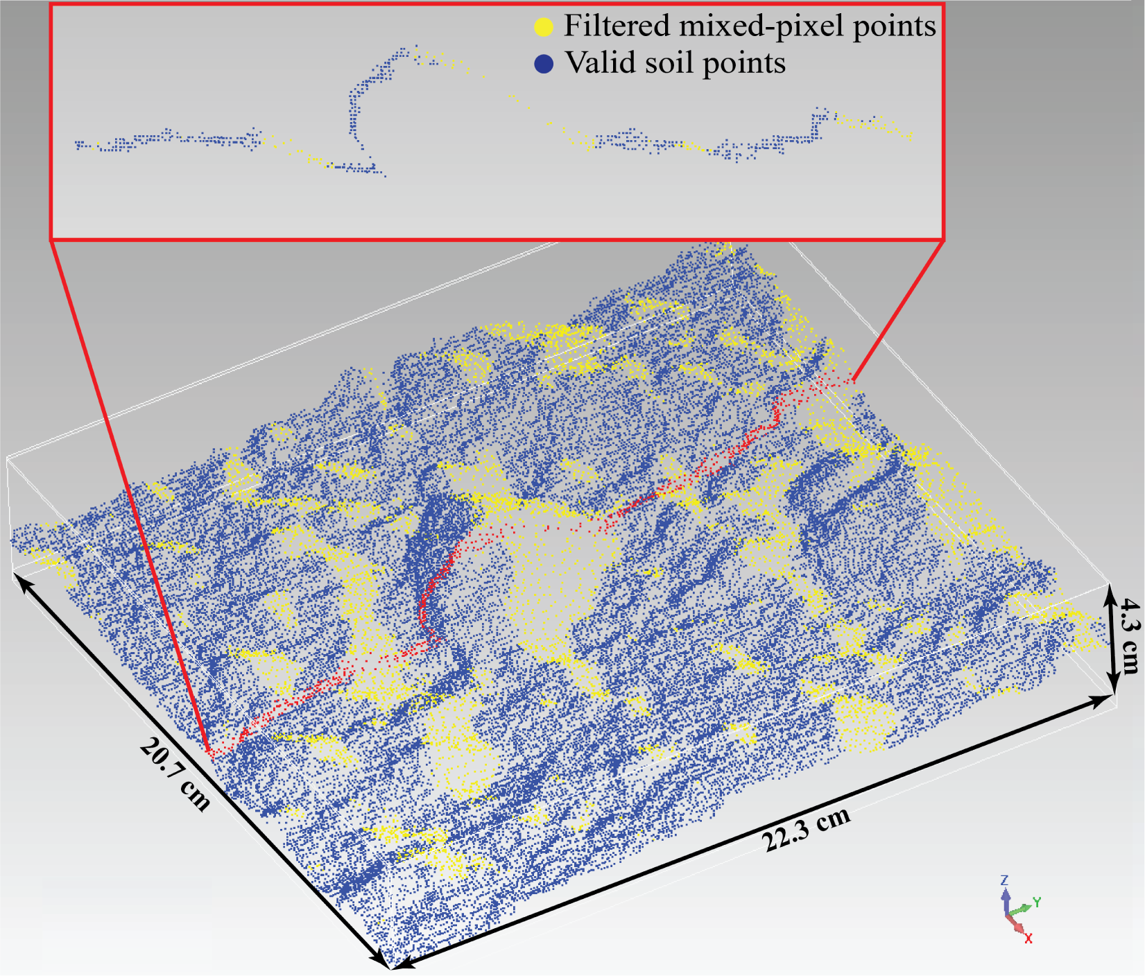
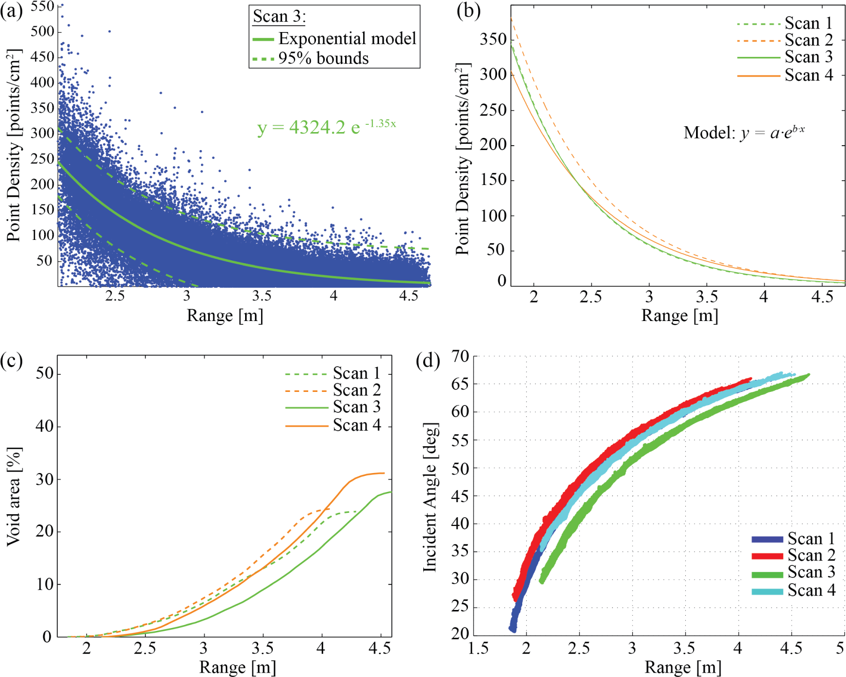
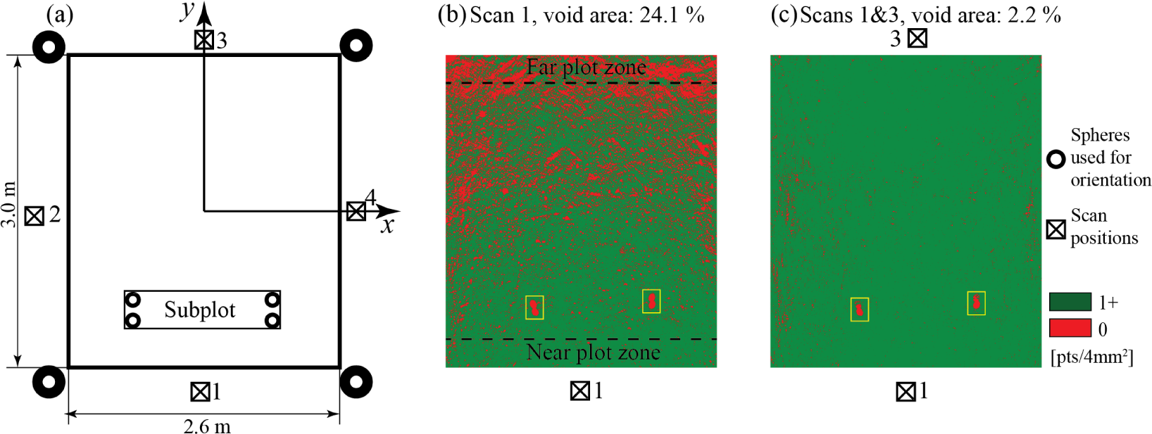


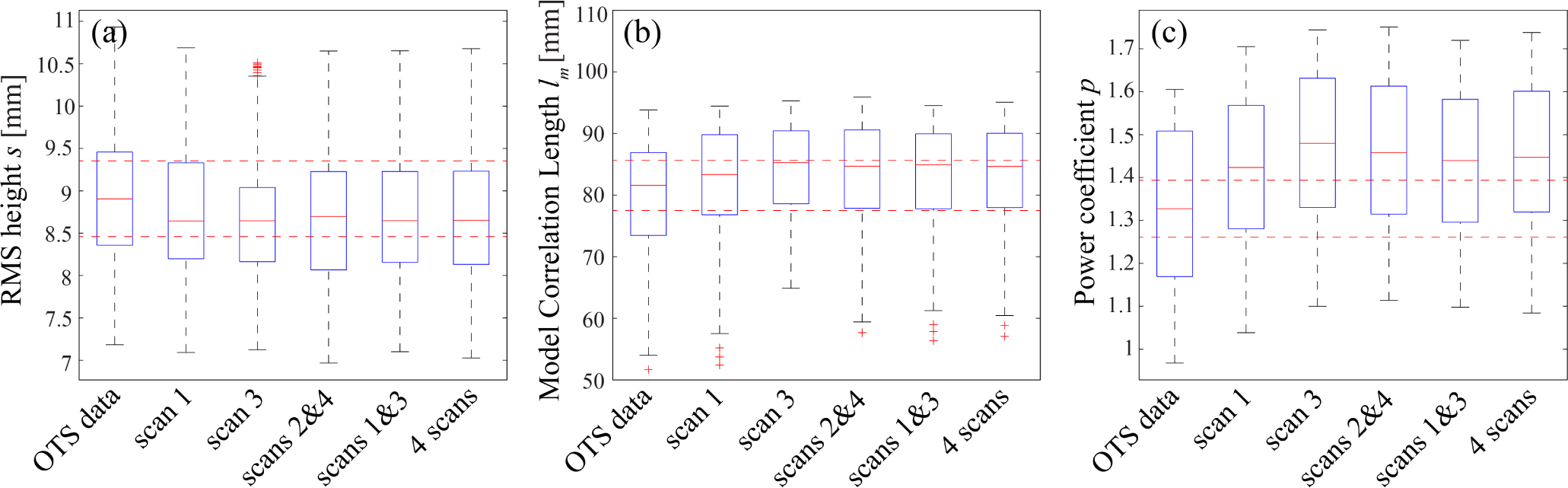
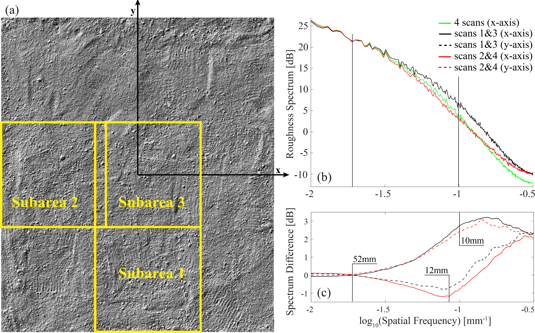

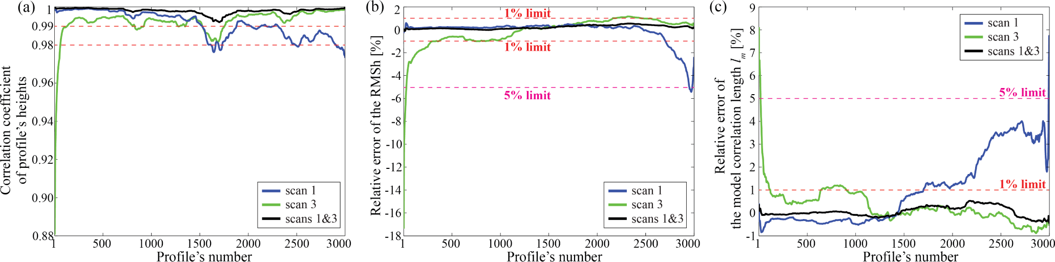
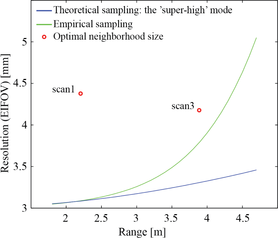

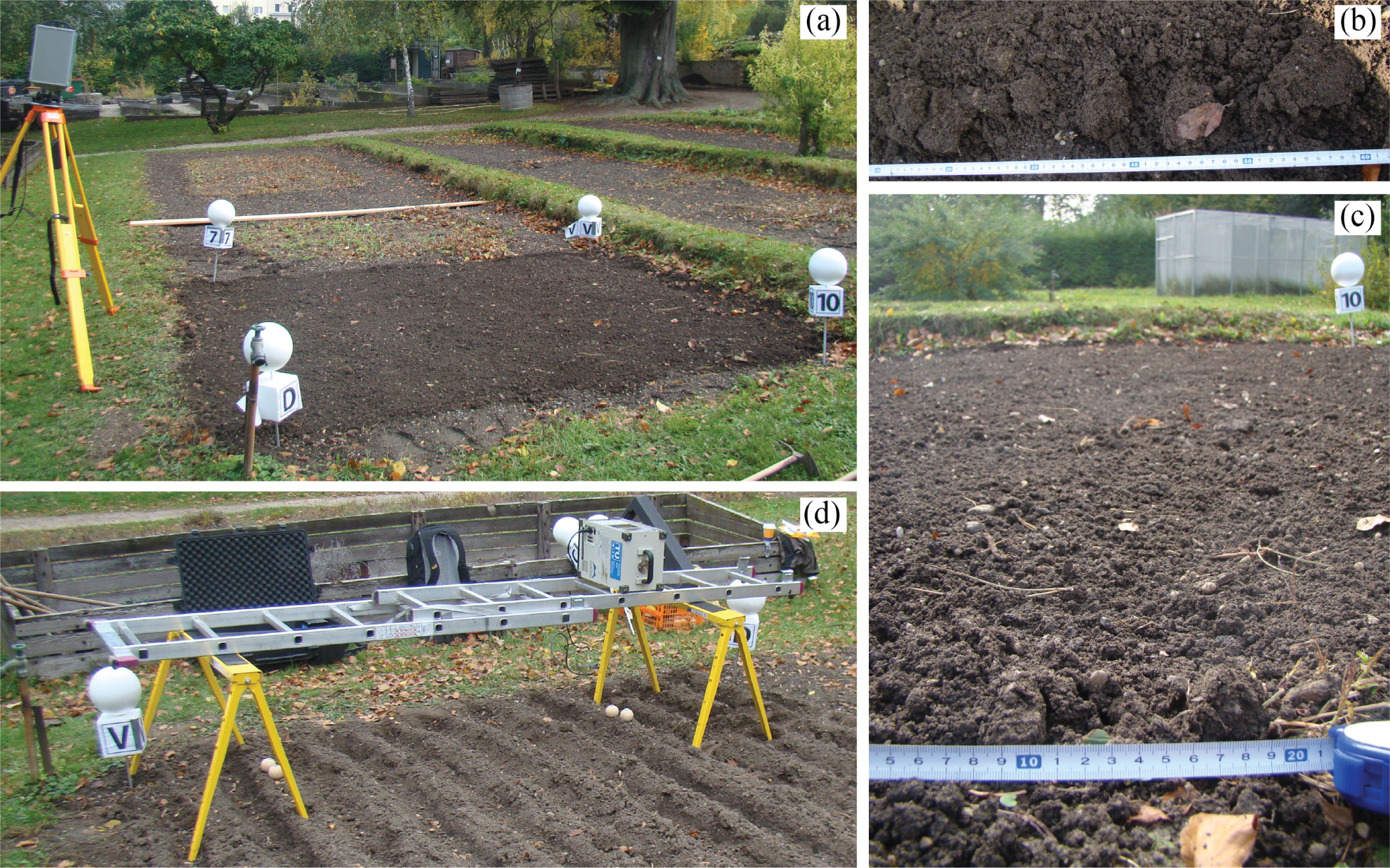
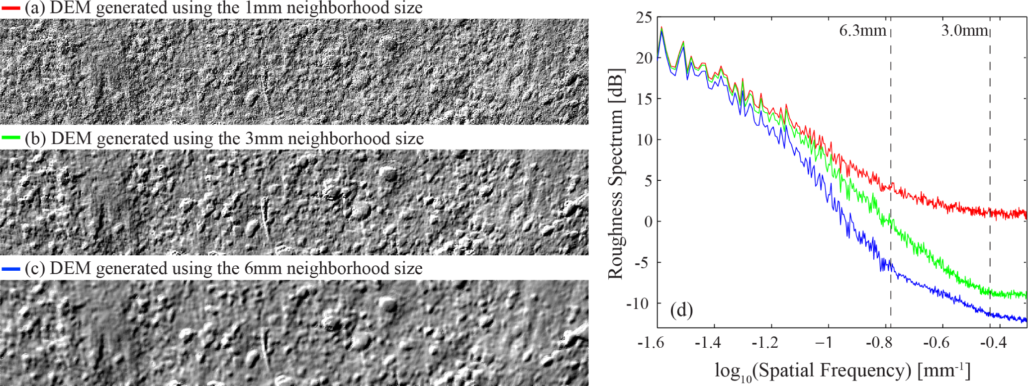
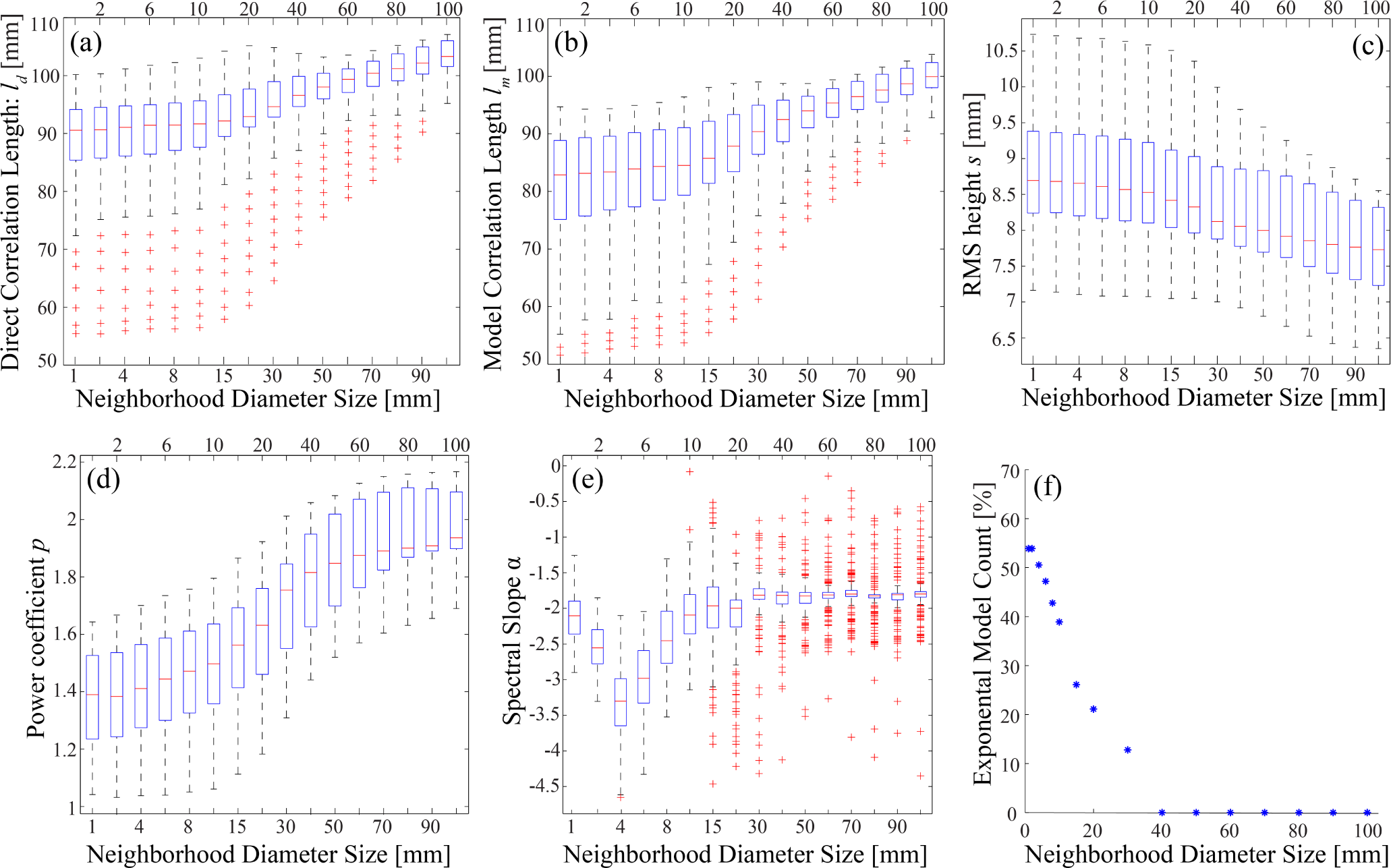
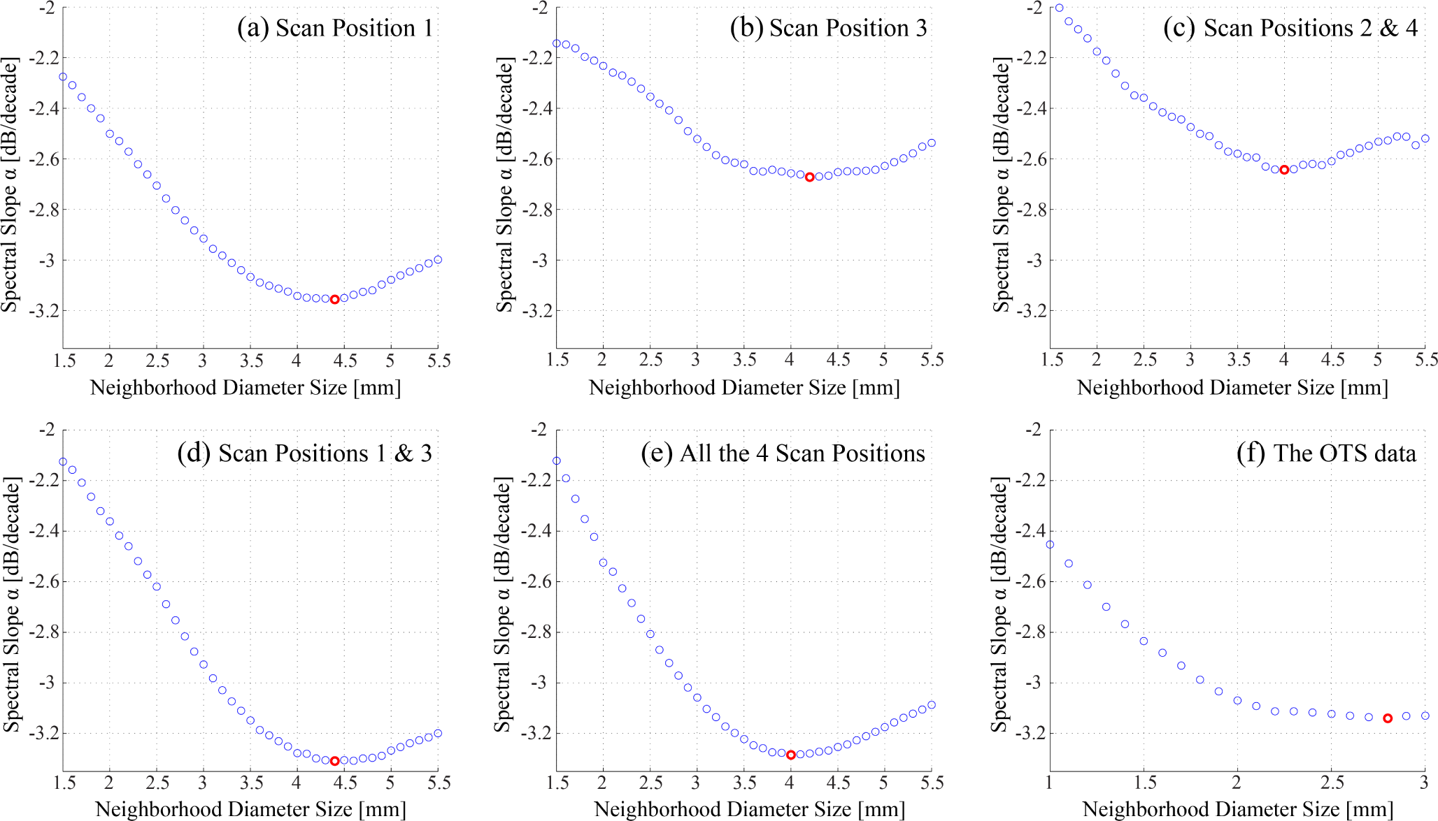
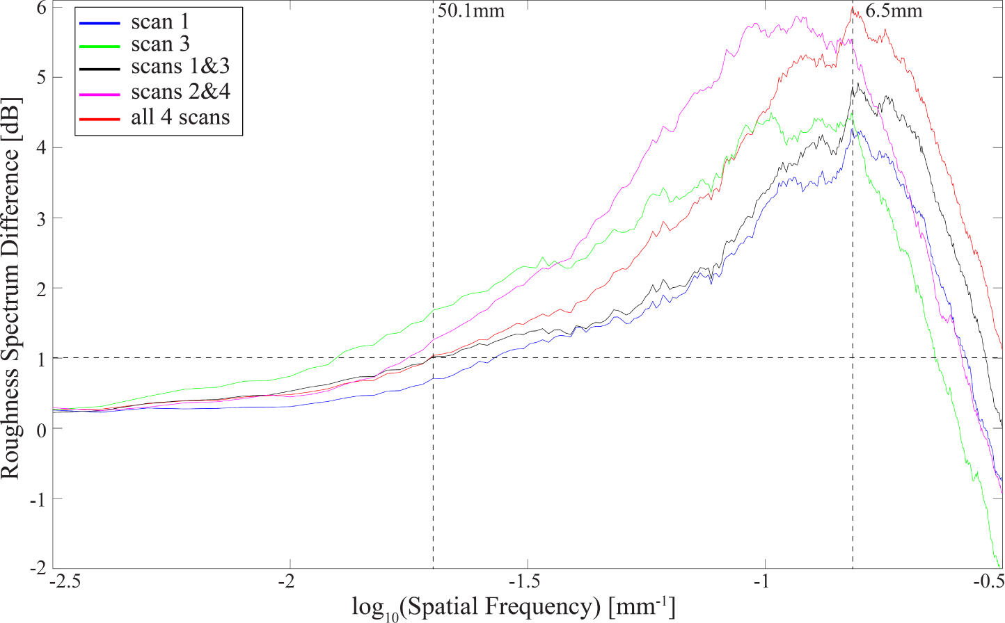
| Name | Range (m)
| Point Density (pts/cm2)
| Sampling Interval (mm)
| Footprint Diameter (mm)
| Sampling Mode* | |||||
|---|---|---|---|---|---|---|---|---|---|---|
| min | mean | max | near | far | near | far | near | far | far | |
| Scan 1 | 1.840 | 2.915 | 4.303 | 251 | 22 | 0.6 | 2.1 | 3.0 | 3.1 | 1.5 |
| Scan 2 | 1.871 | 2.880 | 4.116 | 233 | 21 | 0.7 | 2.2 | 3.0 | 3.1 | 1.4 |
| Scan 3 | 2.127 | 3.276 | 4.664 | 194 | 18 | 0.7 | 2.4 | 3.0 | 3.2 | 1.3 |
| Scan 4 | 2.135 | 3.196 | 4.530 | 159 | 14 | 0.8 | 2.7 | 3.0 | 3.2 | 1.2 |
*The sampling mode is the ratio of the laser footprint diameter to the sampling interval.
| Name | Objective | Section | Data Source | Used Scans | Analyzed Area | Profiling | Neighb. 1 | DEMs 2 |
|---|---|---|---|---|---|---|---|---|
| Set 1 | Effects of Neighborhood Size on Soil Roughness | 3.3 | TLS | 4 Scans | subplot (0.18 m × 1 m) | x-axis | 16 | 16 |
| Set 2.1 | Optimization of Neighborhood Size Using Spectral Slope | 3.4 | TLS | Scan 1 | subplot (0.18 m × 1 m) | x-axis | 41 | 41 |
| Set 2.2 | Scan 3 | 41 | 41 | |||||
| Set 2.3 | Scans 1&33 | 41 | 41 | |||||
| Set 2.4 | Scans 2&43 | 41 | 41 | |||||
| Set 2.5 | 4 Scans | 41 | 41 | |||||
| Set 2.6 | OTS | – | 21 | 21 | ||||
| Set 3 | Comparison of Soil Roughness Derived from OTS and TLS | 3.5 | OTS and TLS | Scan 1; Scan 3; 4 Scans Scans 1&3; Scans 2&4 | subplot (0.18 m × 1 m) | x-axis | 1 | 6 |
| Set 4 | TLS Directional Pattern and Profile Sampling | 3.6 | TLS | Scans 1&3; Scans 2&4; 4 Scans | subarea (1 m × 1 m) | x-axis y-axis | 1 | 3 |
| Set 5 | Single vs. Multiple TLS Scanning and Soil Roughness | 3.7 | TLS | Scan 1; Scan 3 Scans 1&3; 4 Scans | plot (2.6 m × 3 m) | x-axis y-axis | 1 | 4 |
1The Neighb. column shows the number of neighborhood sizes used for DEM interpolation;2The DEMs column shows the number of DEMs that the corresponding DEM set contains.3The ampersand indicates that two opposite scans are merged into a single point cloud.
| Name | Range (m)
| Inc. Angle (°)
| ||||
|---|---|---|---|---|---|---|
| min | mean | max | min | mean | max | |
| Scan 1 | 2.097 | 2.177 | 2.273 | 33.9 | 36.7 | 40.0 |
| Scan 2 | 2.576 | 2.935 | 3.378 | 49.0 | 54.5 | 60.2 |
| Scan 3 | 3.844 | 3.932 | 4.026 | 60.5 | 61.4 | 62.4 |
| Scan 4 | 2.667 | 3.494 | 3.038 | 49.3 | 54.5 | 60.1 |
© 2015 by the authors; licensee MDPI, Basel, Switzerland This article is an open access article distributed under the terms and conditions of the Creative Commons Attribution license (http://creativecommons.org/licenses/by/4.0/).
Share and Cite
Milenković, M.; Pfeifer, N.; Glira, P. Applying Terrestrial Laser Scanning for Soil Surface Roughness Assessment. Remote Sens. 2015, 7, 2007-2045. https://doi.org/10.3390/rs70202007
Milenković M, Pfeifer N, Glira P. Applying Terrestrial Laser Scanning for Soil Surface Roughness Assessment. Remote Sensing. 2015; 7(2):2007-2045. https://doi.org/10.3390/rs70202007
Chicago/Turabian StyleMilenković, Milutin, Norbert Pfeifer, and Philipp Glira. 2015. "Applying Terrestrial Laser Scanning for Soil Surface Roughness Assessment" Remote Sensing 7, no. 2: 2007-2045. https://doi.org/10.3390/rs70202007
APA StyleMilenković, M., Pfeifer, N., & Glira, P. (2015). Applying Terrestrial Laser Scanning for Soil Surface Roughness Assessment. Remote Sensing, 7(2), 2007-2045. https://doi.org/10.3390/rs70202007