
A Regional Land Use Drought Index for Florida


Abstract
:
1. Introduction
2. Dataset
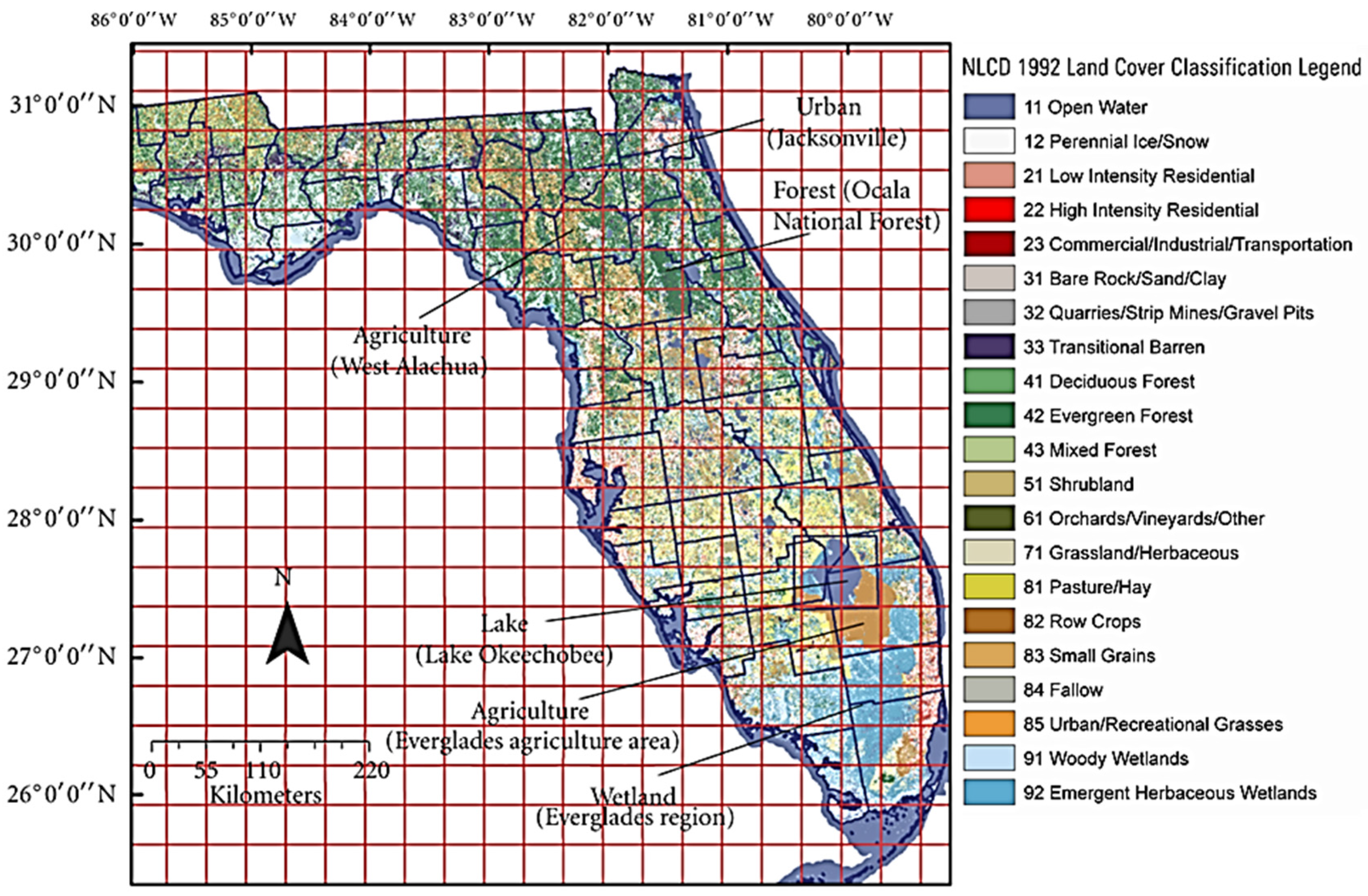
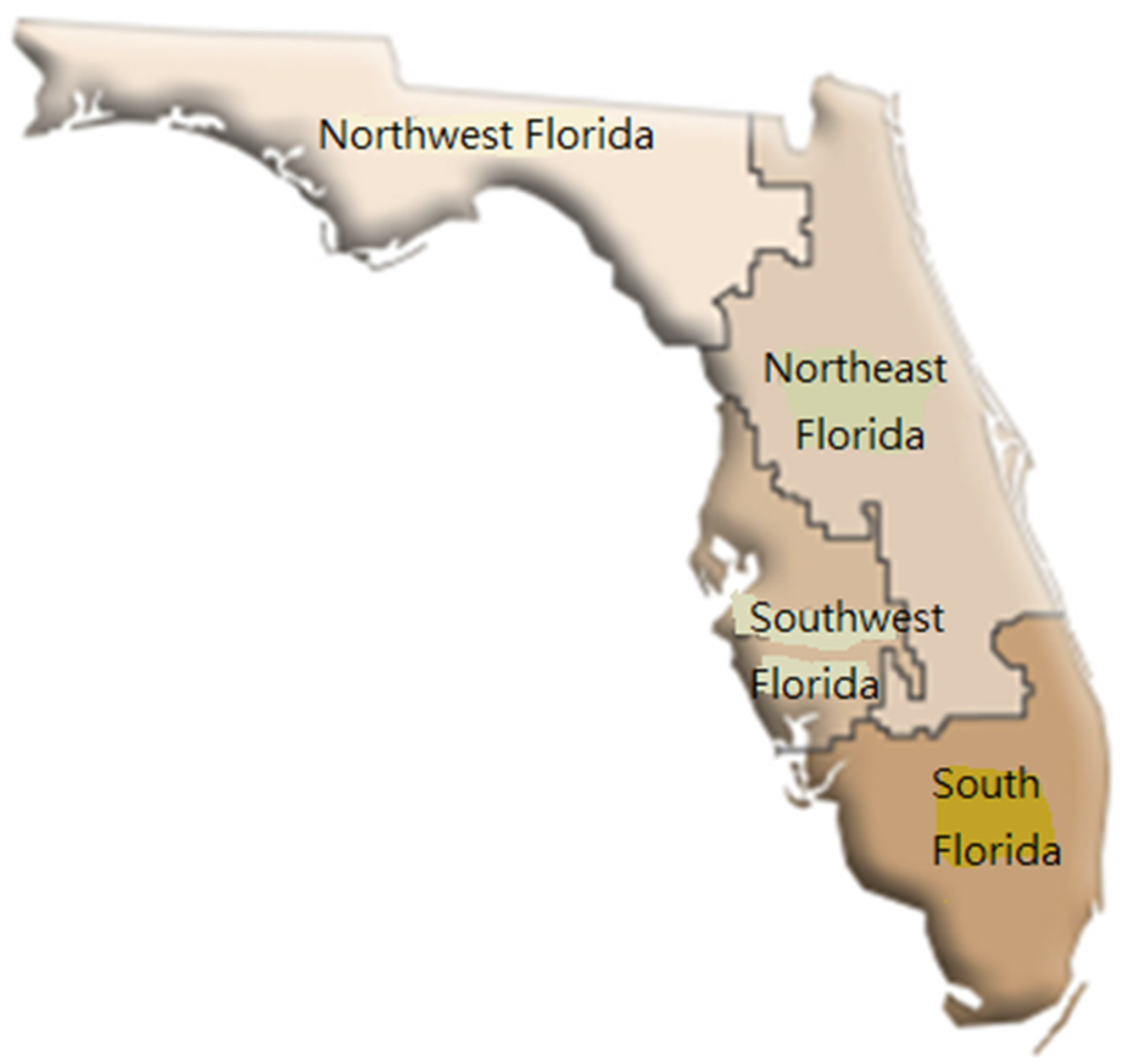
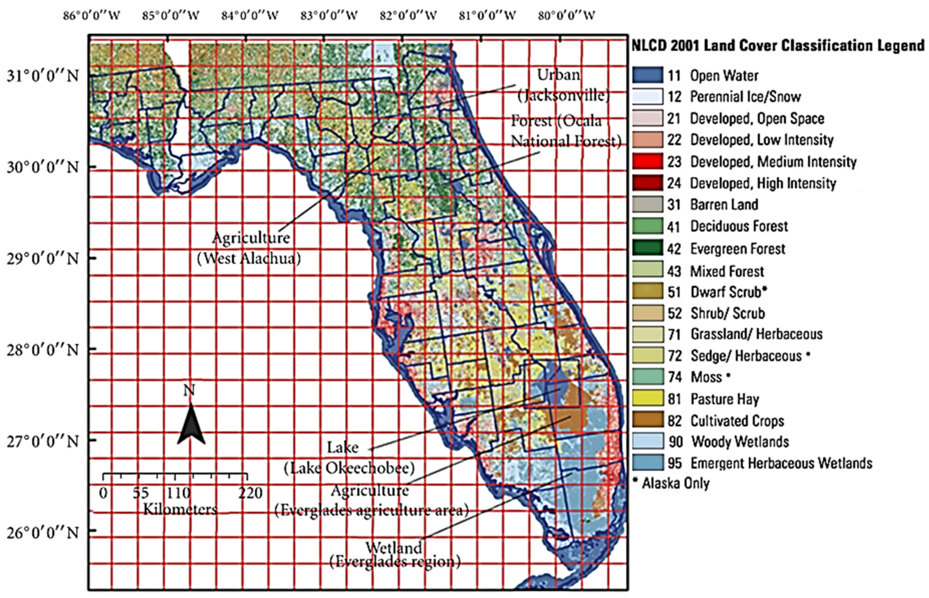
3. Study Area
3.1. ENSO in Florida
3.2. The Selected Areas


4. Methods
5. Result and Discussions
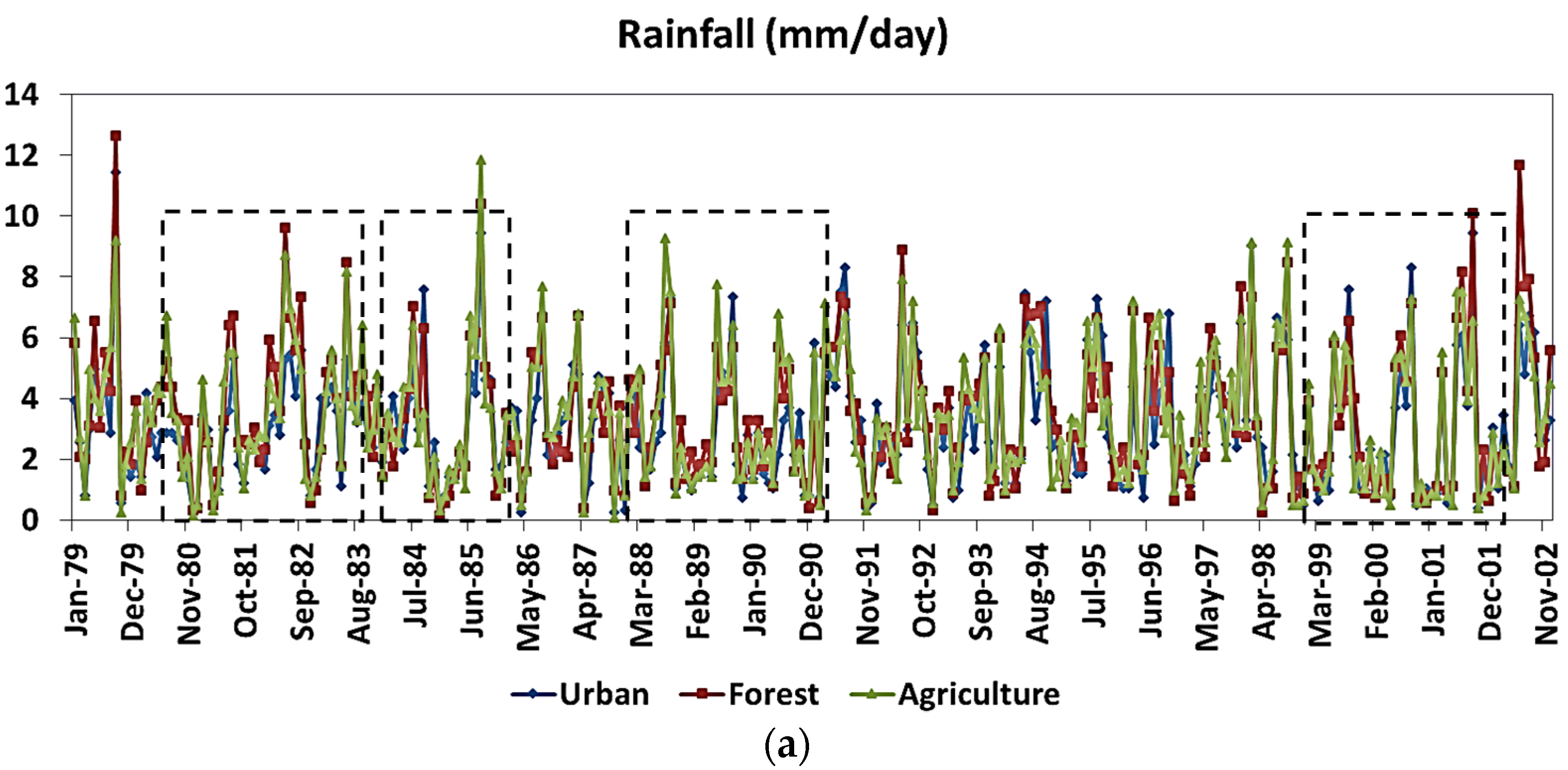
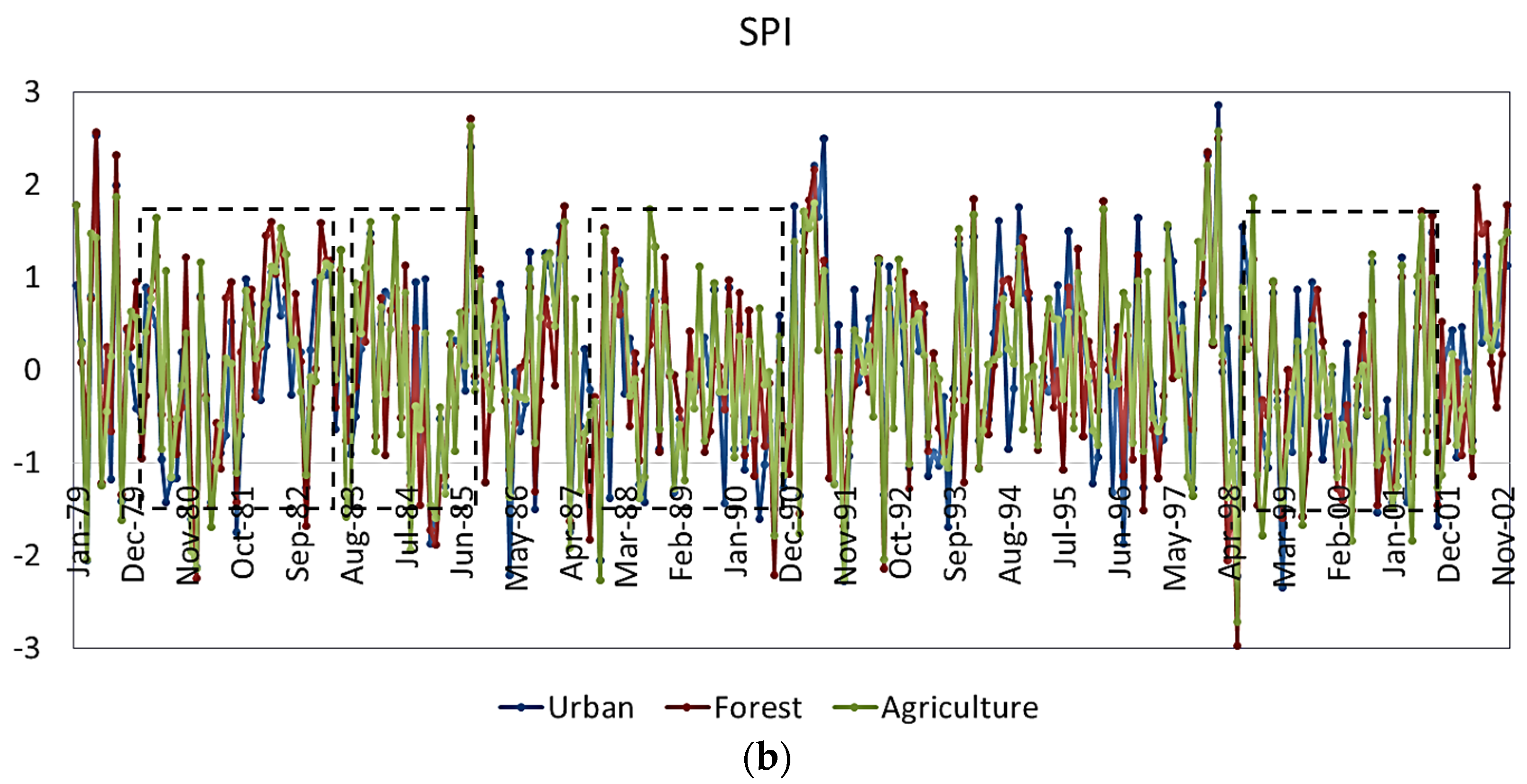
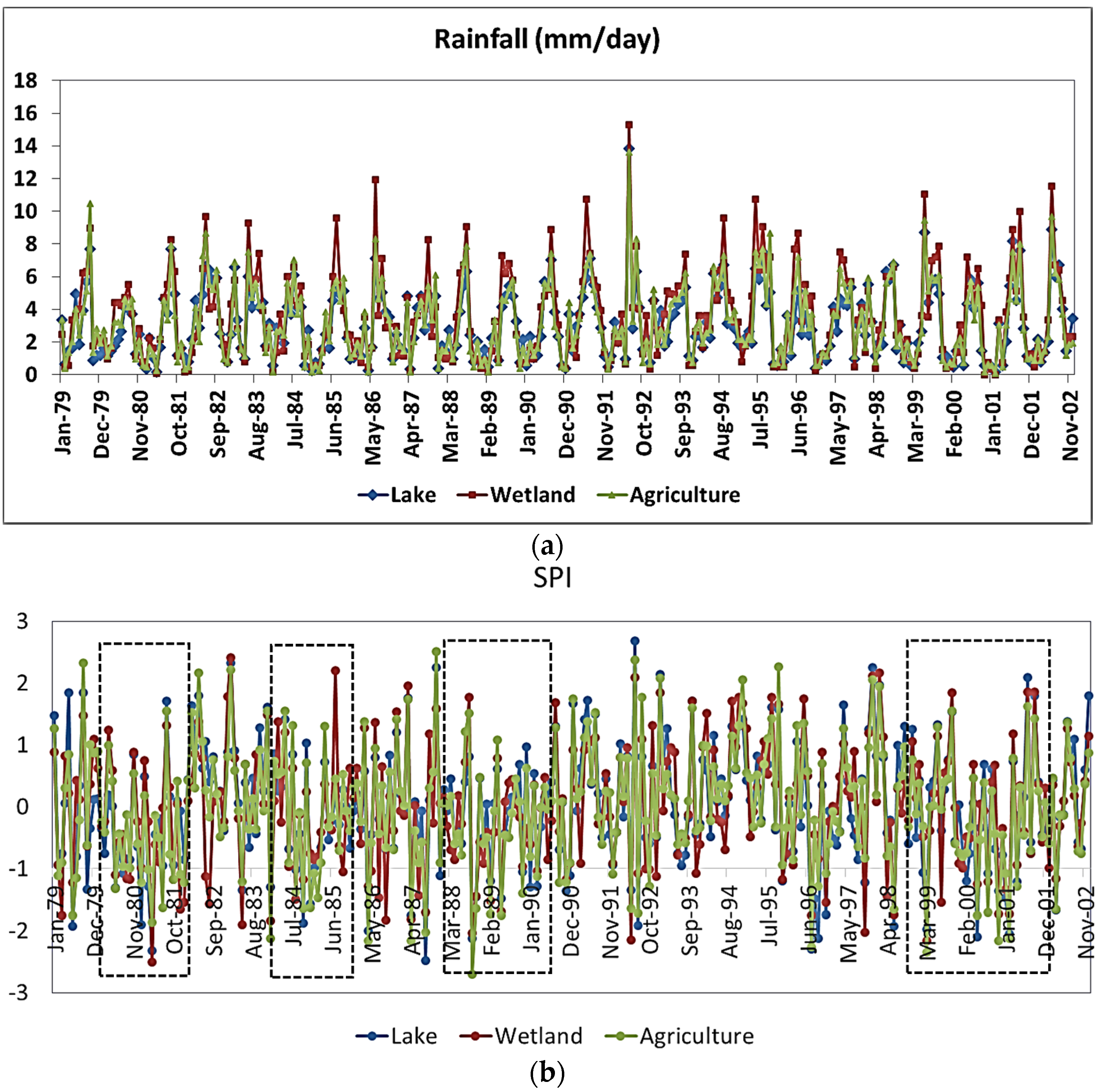
5.1. Monthly Rainfall Variations and Standardized Precipitation Index (SPI)


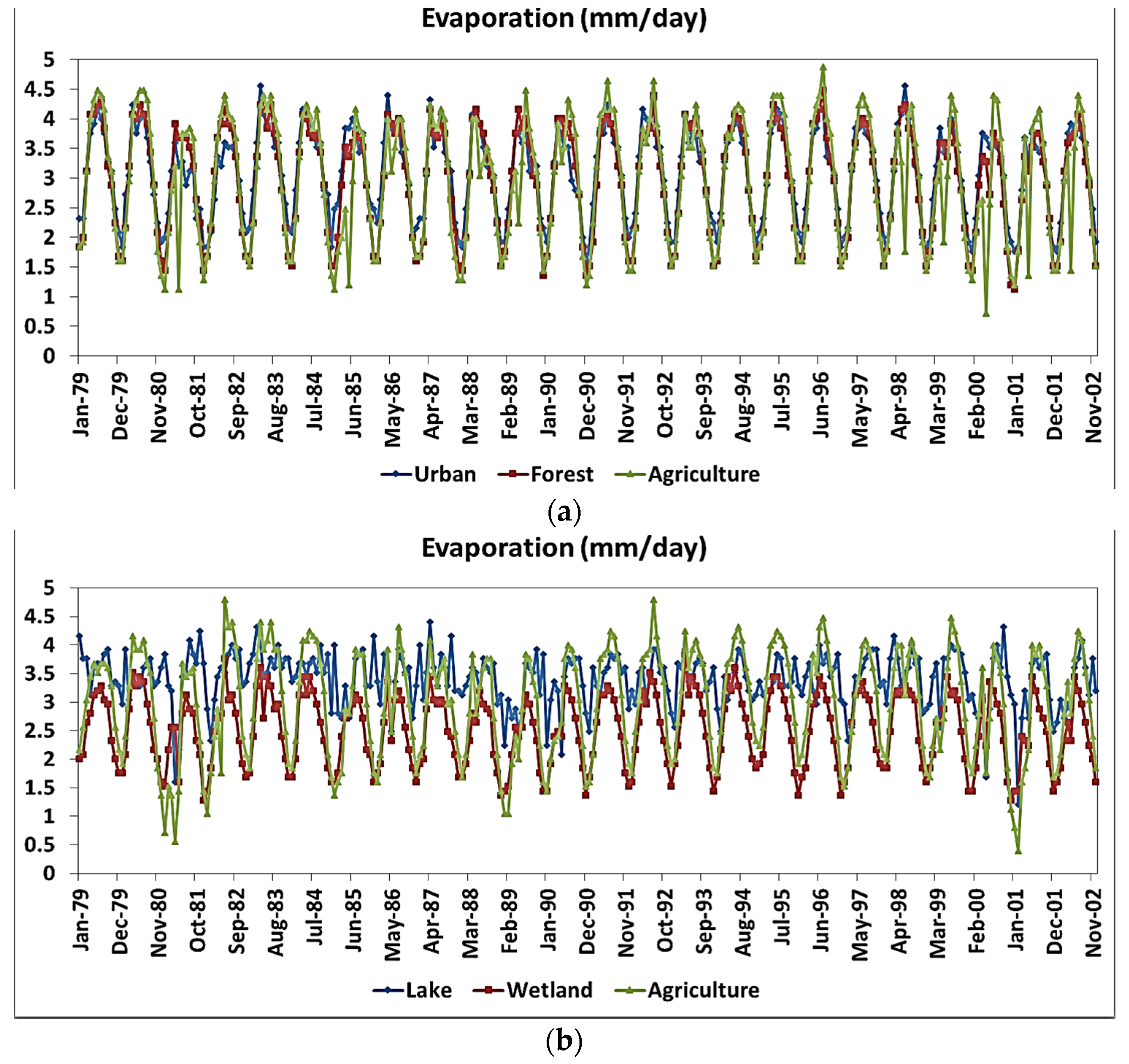
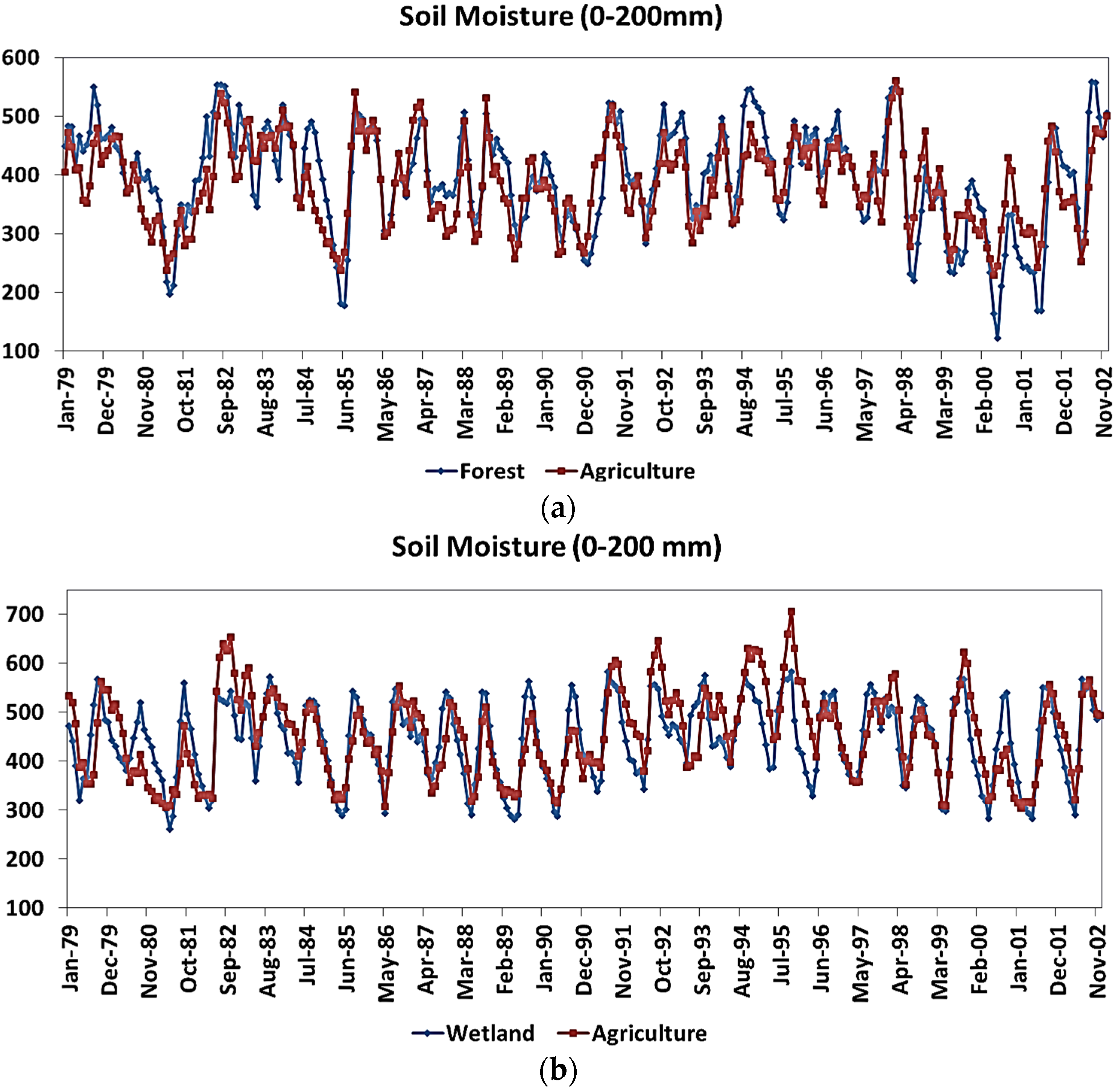
5.2. Monthly Evaporation and Soil Moisture Variations

| 1979–2002 Monthly Average | Rainfall (P) (mm/day) | Evaporation (E) (mm/day) | E/P |
|---|---|---|---|
| Urban | 3.10 | 3.09 | 1.00 |
| Forest | 3.43 | 2.98 | 0.87 |
| Northeast Agriculture | 3.39 | 2.96 | 0.87 |
| Lake | 3.02 | 3.40 | 1.13 |
| Wetland | 3.54 | 2.51 | 0.71 |
| South Agriculture | 3.18 | 2.97 | 0.93 |

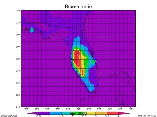
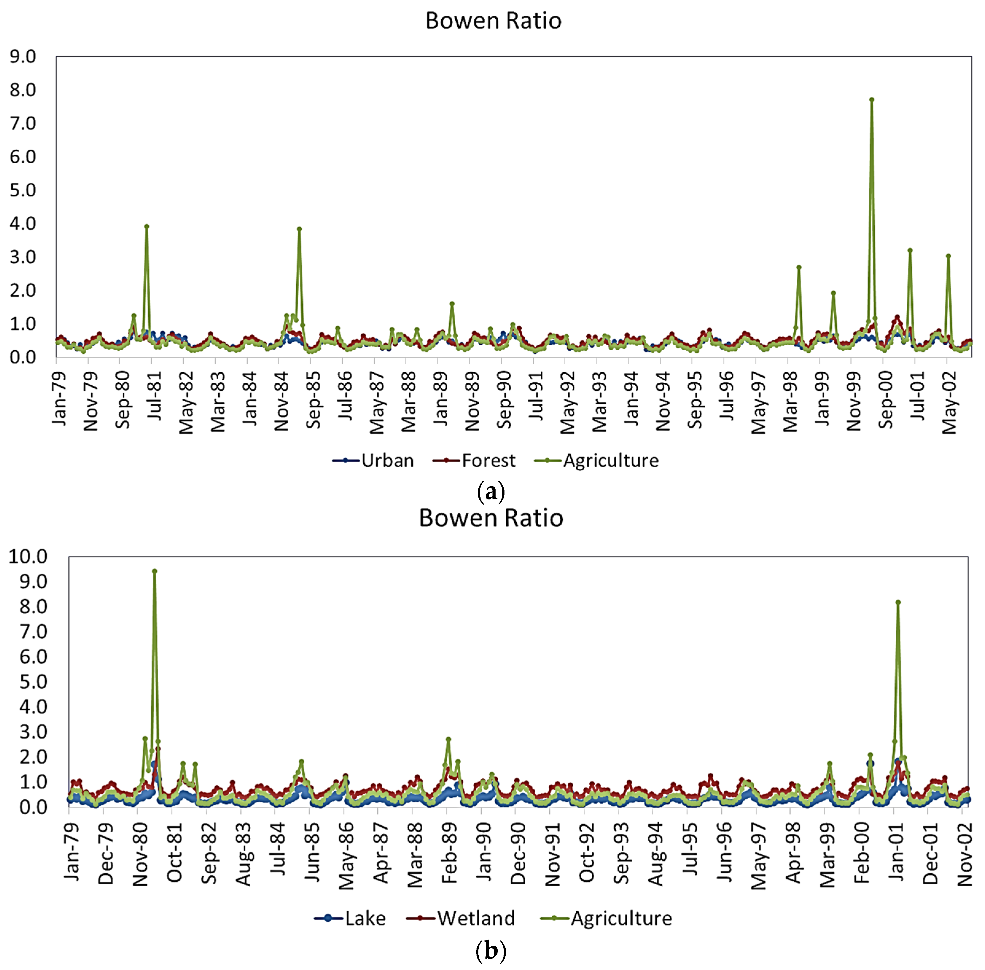
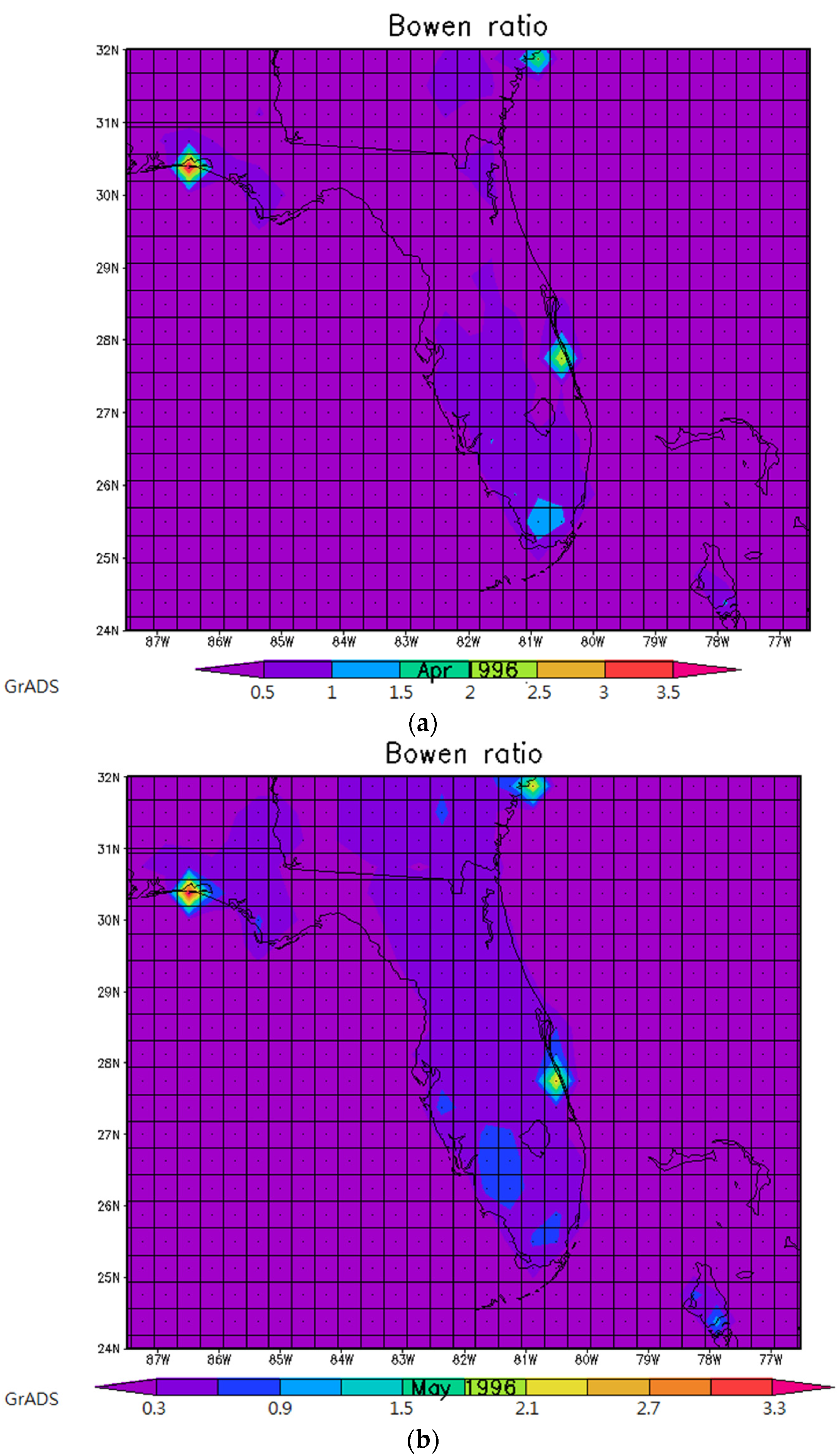
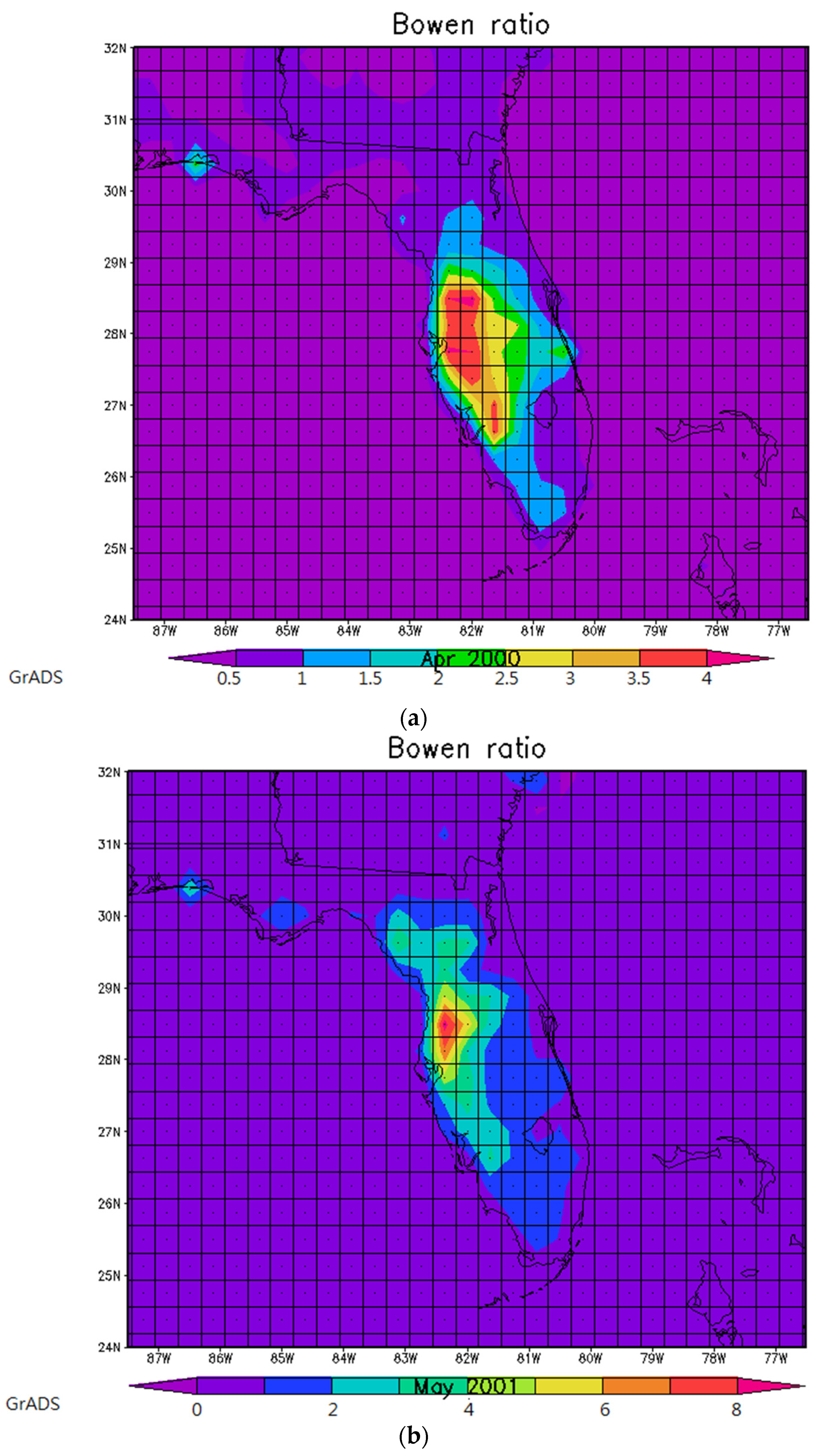
5.3. Monthly Bowen Ratio Variations

| 1979–2002 Monthly Average | Bowen Ratio |
|---|---|
| Urban | 0.44 |
| Forest | 0.49 |
| Northeast Agriculture | 0.51 |
| Lake | 0.33 |
| Wetland | 0.71 |
| South Agriculture | 0.60 |


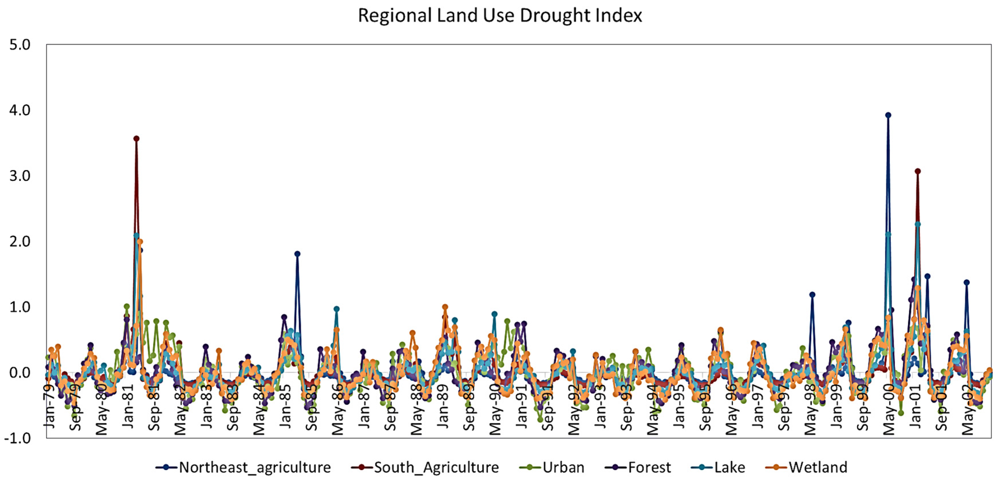
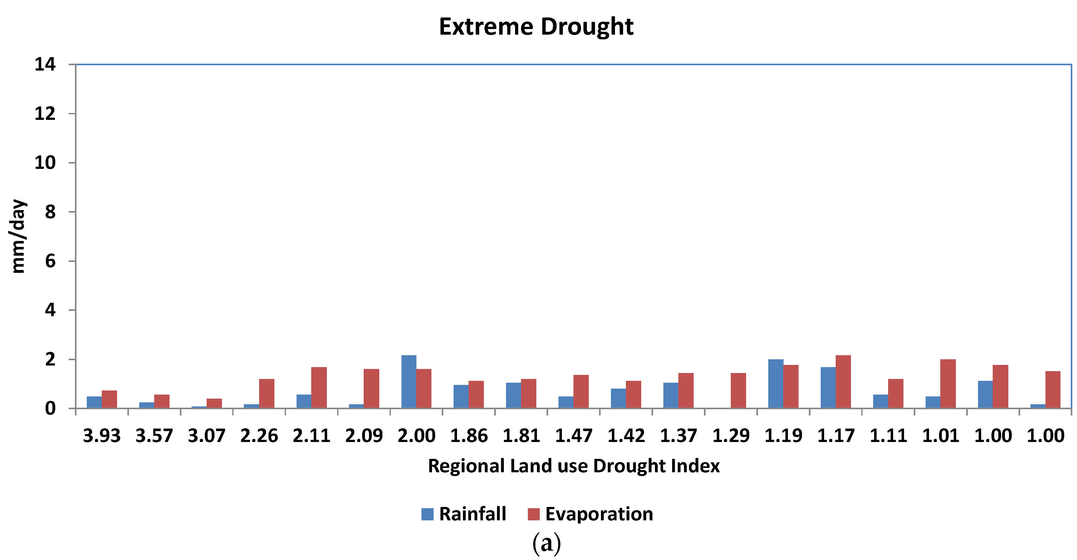
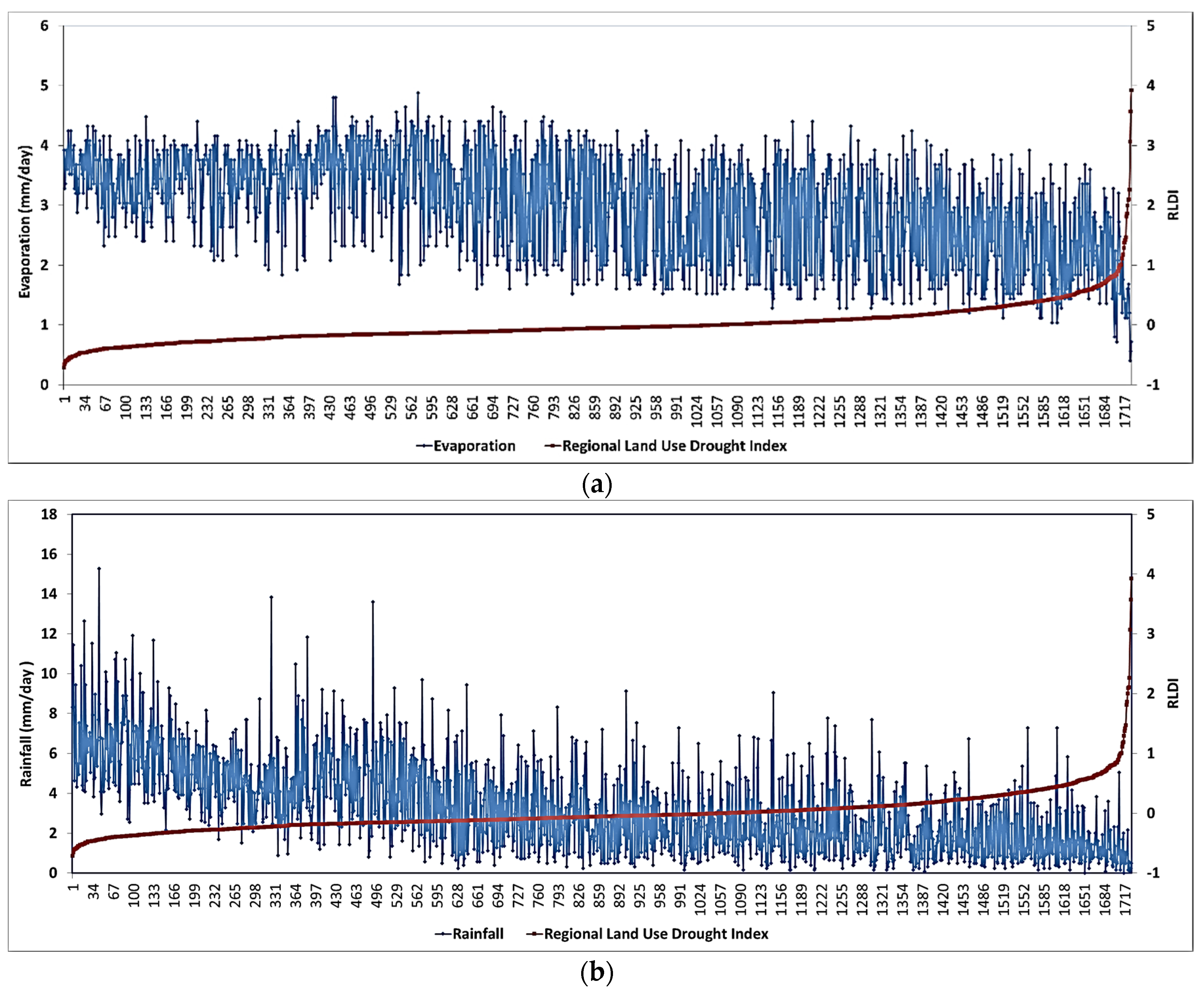
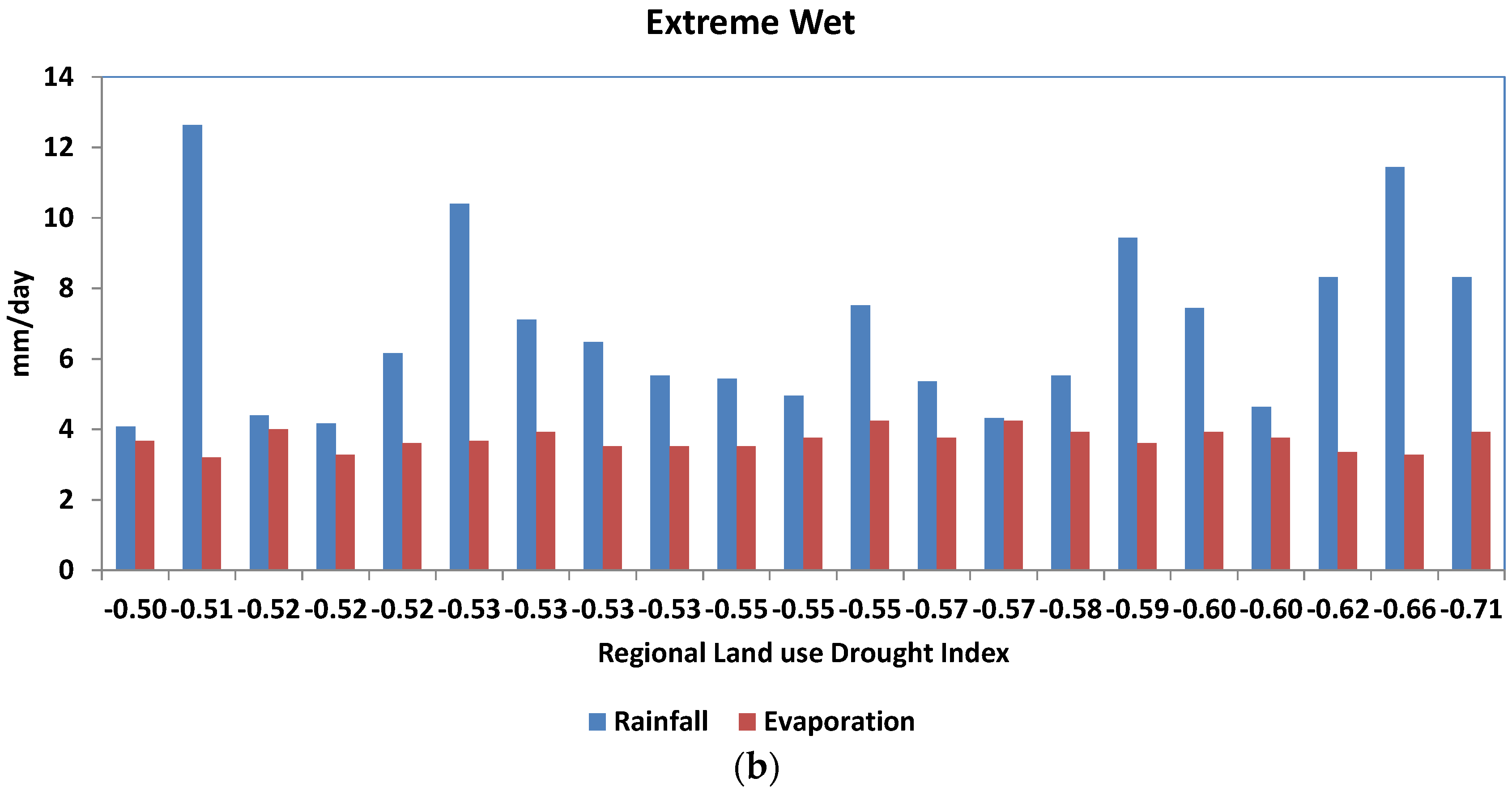
5.4. Regional Land Use Adapted Drought Index (RLDI)
| Drought Classes | Rainfall (mm/day) | Evaporation (mm/day) |
|---|---|---|
| Extreme Drought (RLDI ≥ 1) | 0.74 | 1.36 |
| Moderate drought (0.5 < RLDI < 1) | 1.37 | 2.29 |
| Extreme Wet (RLDI ≤ −0.5) | 6.84 | 3.7 |
| Total average | 3.28 | 2.99 |


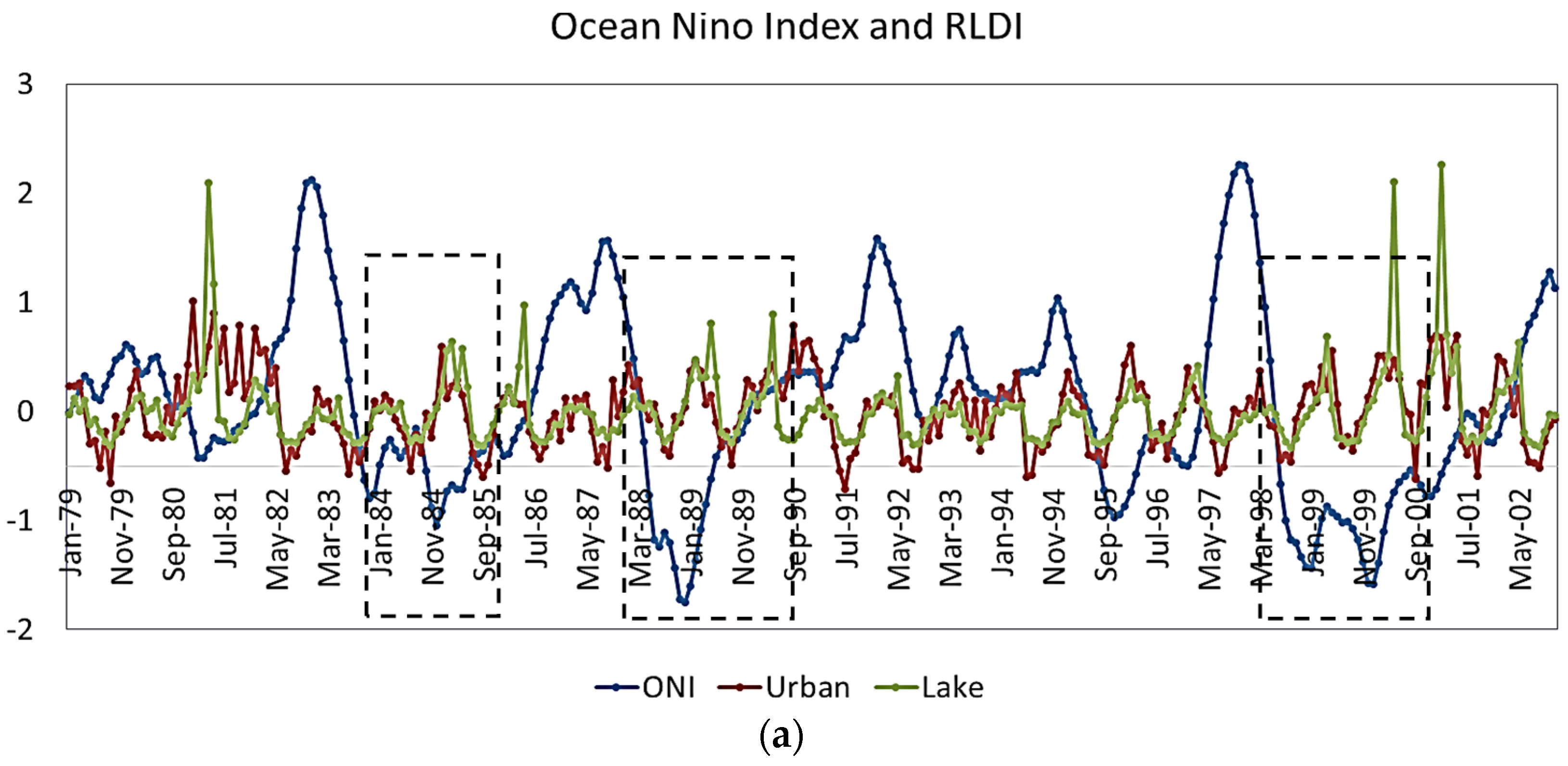
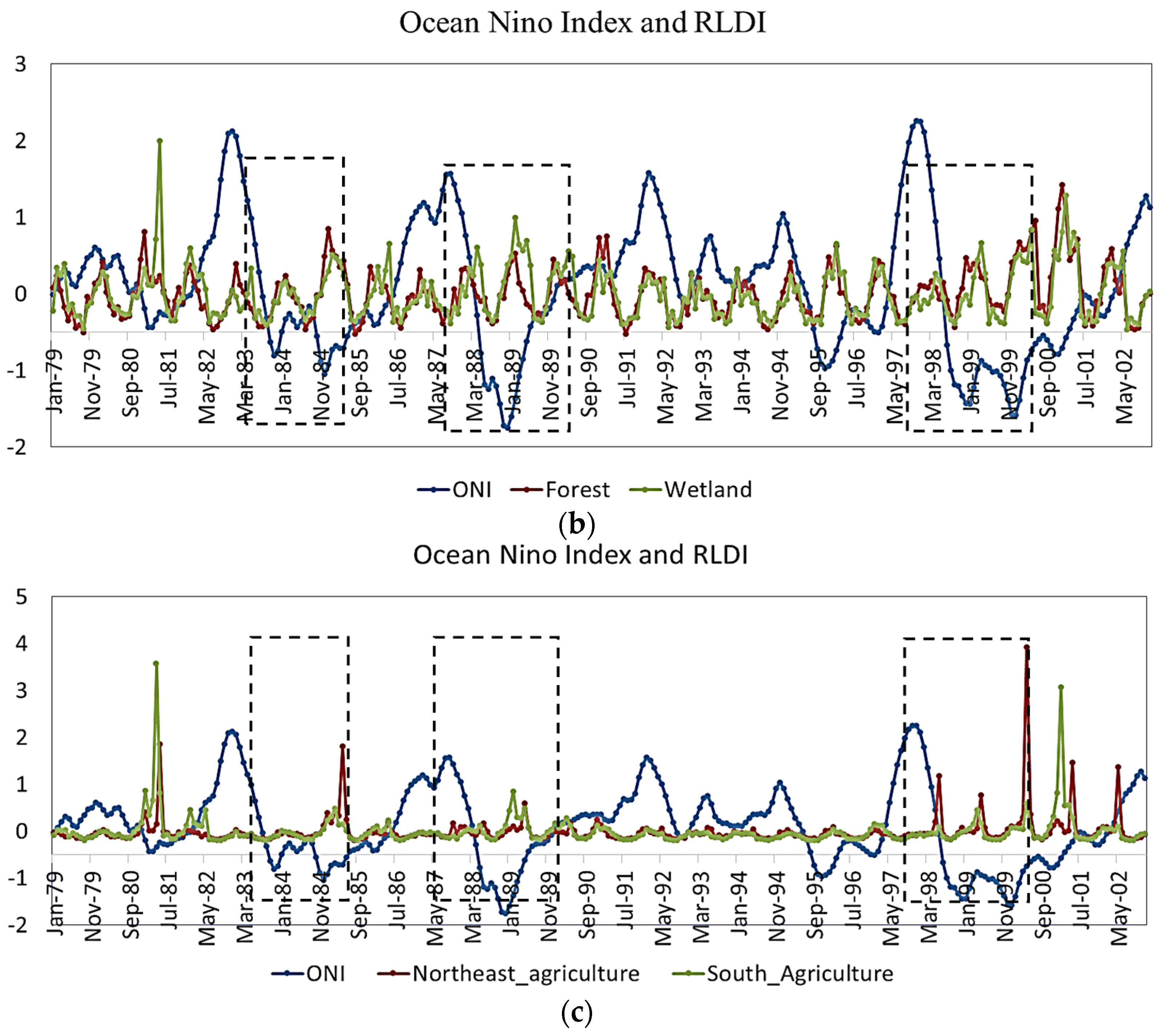
5.5. Oceanic Niño Index (ONI) and RLDI

6. Uncertainties, Errors, and Accuracies
7. Summary and Conclusions
Acknowledgments
Author Contributions
Conflicts of Interest
References
- Nalbantis, I.; Tsakiris, G. Assessment of hydrological drought revisited. Water Resour. Manag. 2009, 23, 881–897. [Google Scholar] [CrossRef]
- Federal Emergency Management Agency, Mitigation Directorate. The 1993 and 1995 Mid-west Floods: Flood Hazard Mitigation through Property Hazard Acquisition and Relocation Program; FEMA Mitigation Directorate: Washington, DC, USA, 1995. [Google Scholar]
- Wilhite, D.A. Drought as a natural hazard: Concepts and definitions. In Drought: A Global Assessment; Routledge: New York, NY, USA, 2000; Volume 1, pp. 3–18. [Google Scholar]
- Palmer, W.C. Meteorological Drought; Weather Bureau Research Paper 45; U.S. Department of Commerce: Washington, DC, USA, 1965. [Google Scholar]
- Palmer, W.C. Keeping track of crop moisture conditions, nationwide: The new crop moisture index. Weatherwise 1968, 21, 156–161. [Google Scholar] [CrossRef]
- McKee, T.B.; Doesken, N.J.; Kleist, J. The relationship of drought frequency and duration to time scales. In Proceedings of the Eighth Conference on Applied Climatology, Anaheim, CA, USA, 17–22 January 1993; American Meteorological Society: Boston, MA, USA, 1993; pp. 179–184. [Google Scholar]
- Shafer, B.A.; Dezman, L.E. Development of a Surface Water Supply Index (SWSI) to assess the severity of drought conditions in snowpack runoff areas. In Proceedings of the 50th Annual Western Snow Conference, Reno, NV, USA, 19–23 April 1982; Colorado State University: Fort Collins, CO, USA, 1982; pp. 164–175. [Google Scholar]
- Thornthwaite, C.W. An approach toward a rational classification of climate. Geogr. Rev. 1948, 38, 55–94. [Google Scholar] [CrossRef]
- Jensen, M.E.; Burman, R.D.; Allen, R.G. Evapotranspiration and Irrigation Water Requirements; ASCE Manuals and Reports on Engineering Practice; American Society of Civil Engineers: New York, NY, USA, 1990. [Google Scholar]
- Abramopoulos, F.; Rosenzweig, C.; Choudhury, B. Improved ground hydrology calculations for global climate models (GCMs): Soil water movement and evapotranspiration. J. Clim. 1988, 1, 921–941. [Google Scholar] [CrossRef]
- Kim, D.; Hi-ryong, B.; Ki-seon, C. Evaluation, modification, and application of the Effective Drought Index to 200-Year drought climatology of Seoul, Korea. J. Hydrol. 2009, 378, 1–12. [Google Scholar] [CrossRef]
- Narasimhan, B.; Srinivasan, R. Development and evaluation of Soil Moisture Deficit Index (SMDI) and Evapotranspiration Deficit Index (ETDI) for agricultural drought monitoring. Agric. For. Meteorol. 2005, 133, 69–88. [Google Scholar] [CrossRef]
- Tsakiris, G.; Vangelis, H. Establishing a drought index incorporating evapotranspiration. Eur. Water 2005, 9, 3–11. [Google Scholar]
- Keyantash, J.A.; Dracup, J.A. An aggregate drought index: Assessing drought severity based on fluctuations in the hydrologic cycle and surface water storage. Water Resour. 2004, 40, 1–14. [Google Scholar] [CrossRef]
- Pan, M.; Wood, E.F. Data Assimilation for estimating the terrestrial water budget using a constrained ensemble kalman filter. J. Hydrometeorol. 2006, 7, 534–547. [Google Scholar] [CrossRef]
- Luo, Y.; Ernesto, H.B.; Kenneth, E.M. The operational ETA model precipitation and surface hydrologic cycle of the Columbia and Colorado Basins. J. Hydrometeorol. 2005, 6, 341–370. [Google Scholar] [CrossRef]
- Findell, K.; LShevliakova, E. Modeled impact of anthropogenic land cover change on climate. J. Clim. 2007, 20, 3621–3634. [Google Scholar] [CrossRef]
- Ek, M.B.; Mitchell, K.E.; Lin, Y.; Grunmann, P.; Rogers, E.; Gayno, G.; Koren, V.; Tarpley, J.D. Implementation of Noah land surface model advances in the National Centers for Environmental Prediction operational mesoscale Eta model. J. Geophys. Res. 2003, 108. [Google Scholar] [CrossRef]
- Mitchell, K. NCEP completes 25-year North American Reanalysis: Precipitation assimilation and land surface are two hallmarks. GEWEX News 2004, 14, 9–12. [Google Scholar]
- Kumar, V.; Panu, U. Predictive assessment of severity of agricultural droughts based on agro-climatic factors. J. Am. Water Resour. Assoc. 1997, 33, 1255–1264. [Google Scholar] [CrossRef]
- Diffenbaugh, N.S.; Giorgi, F.; Pal, J.S. Climate change hotspots in the United States. Geophys. Res. Lett. 2008, 35. [Google Scholar] [CrossRef]
- Dominguez, F.; Kumar, P.; Vivoni, E.R. Precipitation recycling variability and ecoclimatological stability—A study using NARR data. Part II: North American Monsoon Region. J. Clim. 2008, 21, 5187–5203. [Google Scholar] [CrossRef]
- Fall, S.; Niyogi, D.; Gluhovsky, A.; Pielke, R.A.; Kalnay, E.; Rochon, G. Impacts of land use land cover on temperature trends over the continental United States: Assessment using the North American Regional Reanalysis. Int. J. Climatol. 2010, 30, 1980–1993. [Google Scholar] [CrossRef]
- Ropelewski, C.F.; Halpert, M.S. North American precipitation and temperature patterns associated with the El Nino Southern Oscillation (ENSO). Mon. Weather Rev. 1986, 114, 2352–2362. [Google Scholar] [CrossRef]
- Kiladis, G.N.; Diaz, H.F. Global climatic anomalies associated with extremes in the Southern Oscillation. J. Clim. 1989, 2, 1069–1090. [Google Scholar] [CrossRef]
- Hanson, K.; Maul, G.A. Florida precipitation and the Pacific El Niño, 1895–1989. Fla Sci. 1991, 54, 160–168. [Google Scholar]
- Sittel, M.C. Marginal Probabilities of the Extremes of ENSO Events for Temperature and Precipitation in the Southeastern United States; Center for Ocean-Atmospheric Studies, The Florida State University: Tallahassee, FL, USA, 1994. [Google Scholar]
- Twine, T.E.; Christopher, J.K.; Jonathan, A.F. Effects of El Niño-Southern Oscillation on the climate, water balance, and stream-flow of the Mississippi River Basin. J. Clim. 2005, 18, 4840–4861. [Google Scholar] [CrossRef]
- Douglas, A.; Englehart, P. On a statistical relationship between autumn rainfall in the central equatorial Pacific and subsequent winter precipitation in Florida. Mon. Weather Rev. 1981, 109, 2377–2382. [Google Scholar] [CrossRef]
- Florida Agricultural Statistics Service. Florida Agriculture: Vegetables Winter Acreage; Florida Agricultural Statistics Service, Florida Department of Agriculture and Consumer Services: Tallahassee, FL, USA, 1996. [Google Scholar]
- Florida Agricultural Statistics. Florida Agricultural Statistics: Vegetable Summary (1995–1996); Florida Agricultural Statistics Service, Florida Department of Agriculture and Consumer Services: Tallahassee, FL, USA, 1997. [Google Scholar]
- Mills, D.M. Climate change, extreme weather events, and us health impacts: What can we say? J. Occup. Environ. Med. 2009, 51, 26–32. [Google Scholar] [CrossRef] [PubMed]
- Carter, D.R.; Jokela, E.J. Florida’s Renewable Forest Resources; University of Florida Cooperative Extension Service, Institute of Food and Agricultural Sciences: Gainesville, FL, USA, 2002. [Google Scholar]
- Cheng, C.H.; Nnadi, F.; Liou, Y.A. Energy budget on various land use areas using reanalysis data in Florida. Adv. Meteorol. 2014, 2014. [Google Scholar] [CrossRef]
- Folks, J.C. Lake Okeechobee TMDL: Technologies and Research; North Carolina State University College of Agriculture and Life Sciences: Raleigh, NC, USA, 2005; pp. 1–12. [Google Scholar]
- Snyder, G.H. Agricultural Flooding of Organic Soils; Bulletin No. 570; Institute of Food and Agricultural Sciences, University of Florida: Gainesville, FL, USA, 1987. [Google Scholar]
- Drummond, M.A.; Loveland, T.R. Land-use pressure and a transition to forest-cover loss in the Eastern United States. Bioscience 2010, 60, 286–298. [Google Scholar] [CrossRef]
- Knowles, L. Estimation of Evapotranspiration in the Rainbow Springs and Silver Springs Basins in North Central Florida; Technical Report for US Geological Survey, Water Resources Investigations Report 96–4024; U.S. Department of the Interior: Tallahassee, FL, USA, 1996. [Google Scholar]
- Romero, C.C.; Dukes, M.D. Turfgrass and Ornamental Plant Evapotranspiration and Crop Coefficient Literature Review; Agricultural and Biological Engineering Department, University of Florida: Gainesville, FL, USA, 2009. [Google Scholar]
- Viessman, W.; Klapp, J.W.; Lewis, G.L.; Harbaugh, T.E. Introduction to Hydrology; Harper and Row: New York, NY, USA, 1977. [Google Scholar]
© 2015 by the authors; licensee MDPI, Basel, Switzerland. This article is an open access article distributed under the terms and conditions of the Creative Commons by Attribution (CC-BY) license (http://creativecommons.org/licenses/by/4.0/).
Share and Cite
Cheng, C.-H.; Nnadi, F.; Liou, Y.-A. A Regional Land Use Drought Index for Florida. Remote Sens. 2015, 7, 17149-17167. https://doi.org/10.3390/rs71215879
Cheng C-H, Nnadi F, Liou Y-A. A Regional Land Use Drought Index for Florida. Remote Sensing. 2015; 7(12):17149-17167. https://doi.org/10.3390/rs71215879
Chicago/Turabian StyleCheng, Chi-Han, Fidelia Nnadi, and Yuei-An Liou. 2015. "A Regional Land Use Drought Index for Florida" Remote Sensing 7, no. 12: 17149-17167. https://doi.org/10.3390/rs71215879
APA StyleCheng, C.-H., Nnadi, F., & Liou, Y.-A. (2015). A Regional Land Use Drought Index for Florida. Remote Sensing, 7(12), 17149-17167. https://doi.org/10.3390/rs71215879