Abstract
The airborne lidar system has been shown to be an effective and reliable method for spatial data collection. Lidar records the coordinates of point and intensity, dependent on range, incident angle, reflectivity of object, atmospheric condition, and several external factors. To fully utilize the intensity of a lidar system, several researchers have proposed correction models from lidar equations. The radiometric correction models are divided into physically-oriented models and data-oriented models. The lidar acquisition often contains multiple flight lines, and the radiation energy of each flight line can be calibrated independently by calibration coefficient. However, the calibrated radiances in the overlapped area have slightly different measurements. These parameters should be implicitly taken into account if calibrating radiances back to reflectance using known calibration targets. This study used a single-strip physically-oriented model to obtain a backscattering coefficient and a data-oriented model to obtain corrected intensity. We then selected homogeneous tie regions in the overlapped areas, and the differences between strips were compensated by gain and offset parameters in multi-strip radiometric block adjustment. The results were evaluated by the radiometric differences. Nine strips were acquired by Rigel Q680i system, and the experimental results showed that the delta intensity and delta backscattering coefficient of tie regions were improved up to 60% after multi-strip block adjustment.
1. Introduction
The airborne full-waveform light detection and ranging (lidar) system is a kind of active sensor that has already proven to be a state-of-the-art technology for high resolution and highly accurate topographic data acquisition with direct determination of the earth surface elevation. It provides both geometric and radiometric information to identify different objects and has been extensively used in various applications, for example digital elevation modeling [1], topographic mapping [2,3], land cover recognition [4,5,6], and three-dimensional object modeling [4,7,8,9]. In large area topographic mapping, lidar acquisition missions usually contain multiple overlapped flight lines; thus, strip adjustment for multiple lidar strips was developed to ensure the geometrical consistence between strips [10,11,12]. Most previous studies focused on geometric strip adjustment, but the availability of radiometric strip processing for airborne laser scanning is sparse.
In recent years, topographic multi-wavelength lidar systems have been developed to obtain information using different wavelengths. For example, Optech Titan multispectral lidar system uses three independent wavelengths (i.e., 532 nm visible, 1064 nm infrared (IR), 1550 nm near infrared (NIR)) in topographic mapping [13,14]. The multi-wavelength lidar system can be used in atmospheric processing [15], fire detection [16], and geological analysis [17]. However, the lidar radiation is influenced by the reflectivity of the object, material of the target, system factors (i.e., automatic gain control), geometric factors between the sensor and target (i.e., range and incident angle), atmospheric conditions, and several external factors. Therefore, radiometric information from different wavelengths must be calibrated to obtain uniform physical information [18].
Lidar systems not only determine three-dimensional spatial coordinates by direct georeferencing technique, but also provide radiometric properties from active sensors, such as intensity, amplitude, and backscatter cross-section. Wagner et al. (2006) [19] developed lidar equations for waveform lidar and presented the theoretical considerations for backscatter cross-section estimation for radiometric calibration. Wagner (2010) [18] performed radiometric calibration and considered the backscattering coefficient as an additional physical quantity for ground surface characterization. To obtain calibrated radiometric information for spatial analysis, several studies have proposed radiometric correction and calibration models from lidar equations [20,21,22,23] to provide physical properties from the lidar system. However, the previous studies considered single-strip radiometric processing rather than multi-strip radiometric adjustment.
Radiometric calibration can be implemented by amplitude or intensity. For example, Wagner (2010) [18] performed radiometric calibration based on amplitude (from waveform lidar), whereas Ding et al. (2013) [24] based their calibrations on intensity (from discrete lidar) using an intensity correction model considering range, incident angle, and atmospheric conditions. In addition, the Phong reflection model [25] was also applied to attenuate the effects of strong reflections from water areas.
Owing to the different approaches and difficulties of solving each calibration coefficient, the radiometric correction models of lidar include a physically-oriented model based on lidar equations [18] and a data-oriented model based on empirical mathematic functions [26,27,28]. Because asphalt road surface is a more homogeneous reflecting surface than other materials, asphalt roads have been used to derive the radiometric calibration coefficients based on laboratory or in situ measurements [29].
In multi-strip airborne image mosaicking, geometric and radiometric consistencies are two major concerns in the pre-processing stage; geometric consistency relies on bundle-block adjustment, whereas radiometric consistency is based on a color-balance technique. Chandelier et al. [30] proposed a radiometric aerial triangulation method for equalization of digital aerial images that adopts several parameters (i.e., haze variations, temporal differences, and bidirectional reflectance distribution function) that affect the radiation of the images. The purpose of the radiometric model was to minimize the radiometric residuals between images, and the parameters of the radiometric model were determined by the radiometric tie region using a least squares adjustment. Pros et al. [31] presented an image radiometric block adjustment method related to geometric block adjustment to estimate the radiometric gain and offset of sensors, yielding the relation between the at-sensor radiance and the grey-value for each pixel after atmospheric radiative transfer correction. The parameters of the adjustment method were determined by block adjustment through radiometric tie regions.
Inspired by the radiometric correction in digital aerial images, the multi-strip lidar radiometric correction can be implemented using the algorithm from multi-image radiometric correction. Yan et al. [32] found that the lidars taken from different flight lines cannot be mosaicked directly because of intensity discrepancy. They therefore adopted a histogram matching technique from image processing to reduce the intensity discrepancy between strips. The histogram matching technique adjusted the radiometric misalignment between the sub-histograms of the target strip and reference strip to significantly reduce the discrepancy in the normalized intensity image.
Although radiometric correction of single-strip lidar has been recently investigated, the calibrated intensities in the overlapped area are slightly different between strips [32]; therefore, the radiometric correction for multi-strip lidar is needed to obtain uniform radiometric information between strips. Inspired by the radiometric correction of optical images, the concept of radiometric block adjustment can be adopted in multi-strip lidar for radiometric normalization. The challenge of multi-strip radiometric adjustment is to ensure intensity balancing in multiple lidar strips. In other words, multi-strip radiometric adjustment minimizes the radiometrical difference between strips
The aim of this research was to establish an appropriate radiometric block adjustment model for multi-strip airborne waveform and discrete lidars. For waveform lidar, we used the physically-oriented model based on lidar equations in strip-based radiometric correction, and for discrete lidar, we corrected the influences of range and incident angle for intensity in strip-based radiometric correction. After the strip-based correction, radiometric block adjustment based on the data-oriented model was used to improve the radiometric consistence between strips. The scope of this study is to establish a multi-strip radiometric normalization processing for waveform and discrete lidars, a method that may improve the radiometric consistence in multi-strip lidar mosaicking. In addition, the validation of the proposed method included quantitative and qualitative analysis before and after radiometric normalization.
2. Study Area and Dataset
The test area was located in Miaoli city, Taiwan, an area about 6,804,000 m2 (2700 m × 2520 m) (Figure 1) with mixed buildings, farms, and trees. The terrain is flat, and the height of lidar ranges from 60 m to 150 m. The waveform lidar data were obtained on 30 April 2013, by the Rigel LMS-Q680i system at an average flying height of 410 m and included nine overlapping strips (Figure 2). The pulse repetition frequency and scan rate are 300 kHz and 200 lines/s. Besides, the field of view and beam divergence are 60 degrees and 0.5 mrad. The total number of point clouds in the study area was about 114 million, and the average point density was about 16 pts/m2 (Table 1).
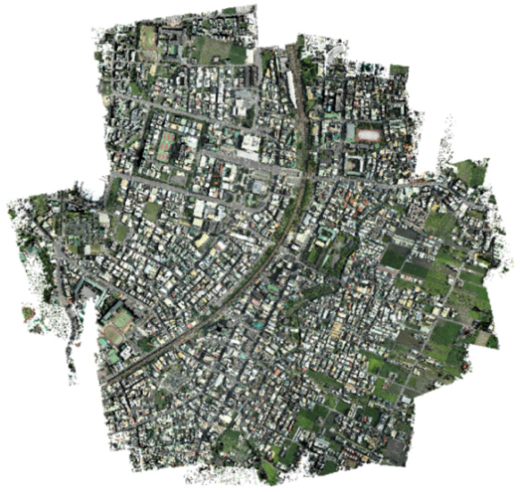
Figure 1.
Test area.
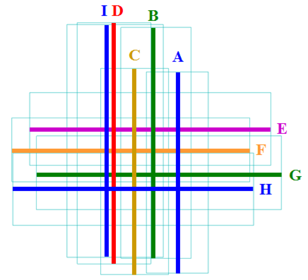
Figure 2.
Nine lidar strips.

Table 1.
Parameters for lidar strip.
| Strip No. | Direction | Height (m) | Length (m) | Swath (m) | Area (m2) | Point | Density | |
|---|---|---|---|---|---|---|---|---|
| A | N to S | 409 | 2019 | 621 | 1,254,503 | 14,624,049 | 11.66 | |
| B | S to N | 379 | 2312 | 703 | 1,625,821 | 11,246,618 | 6.92 | |
| C | N to S | 382 | 2066 | 679 | 1,403,830 | 14,536,123 | 10.35 | |
| D | S to N | 408 | 2416 | 737 | 1,780,059 | 10,289,728 | 5.78 | |
| E | W to E | 420 | 2412 | 729 | 1,759,366 | 11,509,870 | 6.54 | |
| F | E to W | 385 | 2382 | 639 | 1,521,724 | 15,960,908 | 10.49 | |
| G | W to E | 363 | 2451 | 737 | 1,806,575 | 12,383,787 | 6.85 | |
| H | E to W | 370 | 2413 | 726 | 1,750,655 | 15,058,611 | 8.60 | |
| I | S to N | 575 | 2331 | 964 | 2,35,5476 | 7,492,812 | 3.33 | |
| Total | 6,806,076 | 113,102,506 | 16.62 | |||||
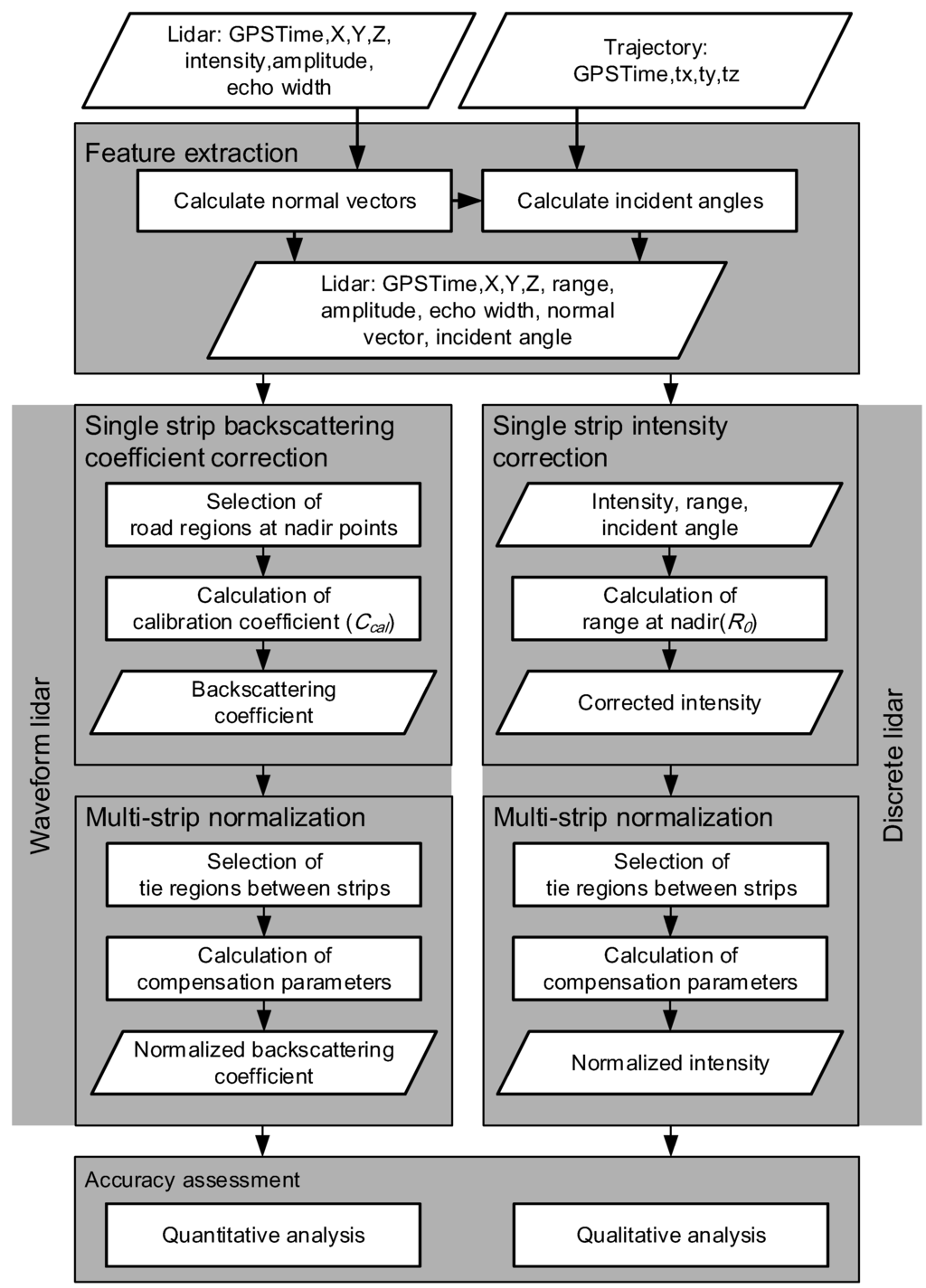
Figure 3.
The workflow of multi-strip radiometric normalization.
3. Proposed Scheme
The workflow (Figure 3) consisted of four major parts: (1) feature extraction; (2) single-strip calibration; (3) multi-strip normalization; and (4) accuracy assessment. First, we extracted the amplitude and echo width from waveform, range, and incidence angle from trajectories, and intensity from LAS file. The LAS file format is a public file format for three-dimensional point clouds [33]. We then obtained the backscattering coefficient from lidar equations and corrected intensity from range/incidence normalization for each strip separately. Several tie regions were selected automatically for radiometric block adjustment to determine radiometric correction parameters (i.e., gain and offset). Finally, we conducted quantitative and qualitative accuracy assessments.
3.1. Feature Extraction
This stage extracts essential parameters for radiometric correction from lidar. The input data included lidar data in LAS [33] and SDW [34] files and trajectory. Each lidar point in the LAS file contains GPS time, X, Y, Z, and original intensity that represent the data source from discrete lidar. The SDW file is the output of waveform lidar using Riegl RiAnalyze. Each lidar point in the SDW file contains GPS time, X, Y, Z, amplitude, and echo width from waveform. The RiAnalyze utilized Gaussian pulse fitting [19] (Equation (1)) to decompose a received waveform into several Gaussian functions; amplitude and echo width were also extracted from the Gaussian function:
where Pr(x) is the received lidar waveform, is the amplitude, is the echo width, is the position of peak, and N is the number of echoes.
Range and incident angle: Because the GPS time is attached in lidar point and trajectory, we used lidar point’s GPS time to determine corresponding trajectory. By comparing the GPS times, the trajectory of each lidar point can be easily determined, and hence the scan range between scanning position and object can be calculated by trajectory and lidar point. Incident angle was the angle between surface normal and laser line-of-sight, an important parameter that reduces the angle effects in radiometric normalization. The surface normal vector was determined by plane fitting from the nearest lidar points within a certain distance in the object space [35]. In this study, the lidar points within a 1 m radius were selected for plane fitting. The surface normal vector can be calculated from plane coefficients after plane fitting. The line-of-sight of laser is calculated from coordinates of lidar point and trajectory. Finally, the incident angle θ can be calculated from the dot product of surface normal vector and laser line-of-sight .
3.2. Single-Strip Calibration
The backscattering coefficients and corrected intensities were calculated to correct systematic biases. The backscattering coefficients were obtained by lidar equations, and asphalt road regions were selected as reference targets. The corrected intensities were normalized from scan range and incident angle.
For backscattering coefficients, the lidar equation was used to calculate the backscattering coefficient via waveform features [18]. The effects of amplitude, echo width, range, and incidence angle were incorporated into backscattering coefficient for each strip. We assumed a reflectance of 0.25 for asphalt road at a wavelength of 1550 nm [21,29] and manually selected asphalt roads located at the nadir point as the reference target. An individual calibration constant, , was calculated for each strip (Equation (2)) and applied to each pulse to obtain the backscattering coefficient (Equation (3)):
where is the calibration constant, is the reflectivity of object (i.e., 0.25 for asphalt road in this study), is the laser beam divergence (i.e., 0.5 mrad for Riegl Q680i in this study), is the scan range, is the amplitude, is the echo width, is the backscatter cross-section, is the backscattering coefficient, is the area of footprint, and is the incidence angle.
The uncorrected intensity in the LAS file was affected by scan range and incident angle. The intensity near the edge was lower than the nadir point; we therefore used scan range and incident angle to obtain a corrected intensity (Equation (6)) [24]:
where is the corrected intensity, is the original intensity, is the scan range, is the range at nadir point, is the atmosphere factor, and is the incidence angle. The corrected intensities eliminate the effects of range and incidence angle and can be an alternative for radiometric correction when the waveform features are not available. After correction, the intensities of the same material (e.g., road) are more uniform at different view directions and ranges (Figure 4).
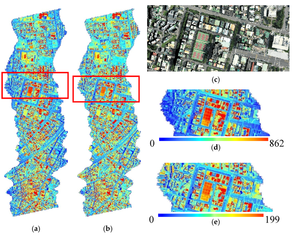
Figure 4.
Illustration of intensity correction: (a) original intensity; (b) corrected intensity; (c) reference image; (d) enlargement of original intensity; and (e) enlargement of corrected intensity.
3.3. Multi-Strip Normalization
Theoretically, the radiance of an object from different flight lines should be the same in the overlapped area. Because not all the system parameters (e.g., internal parameters of the instrument) were considered in the single-strip calibration, the calibrated values (i.e., backscattering coefficients and corrected intensities) were slightly different in the overlapped area. Notice that, these system parameters are implicit in radiometric calibration by calibration targets [2,36]. To calculate and compensate for the difference between strips, we proposed an automatic process for tie region selection. Asphalt road or other homogeneous regions can be selected automatically. Our method selects homogeneous regions based on geometrical and radiometrical properties. The homogeneous criteria include: (1) overlapped area; (2) flatness of a region; and (3) homogeneity of radiometric responds. We consider the overlapped areas in automatic selection of tie regions. The flatness of a region is evaluated by the curvature [37] of a region. A small curvature indicates a planar object like road and roof top. The performance of curvature is better than delta Z as the curvature is able to handle gable roof while delta Z can only extract the horizontal planes. The standard deviation of intensity within a region is also used to select a homogeneous area.
To consider the distribution of tie regions, the study area is divided into 100 sub-regions (10 rows × 10 columns) equally. All the non-overlapped areas are excluded in the selection of tie region. Then, we use a 5 m × 5 m moving window to extract the homogeneous areas within the overlapped areas. If the standard deviation of a curvature and the intensity of a moving window are smaller than the predefined thresholds, this moving window is selected as a homogeneous area. For example, Mi and Mj are overlapped windows in strip i and strip j, respectively. If both Mi and Mj are determined as homogeneous areas, then, these two windows are selected as a candidate tie region. Several candidates can be selected within a sub-region and the one nearest to the center point of a sub-region is selected to represent the tie region in this sub-region. The total number of automatic extracted tie regions is 54 (Figure 5a). Among these 54 tie regions, 40 regions are roads and 14 regions are roofs. The numerical static shows that the proposed method is able to select the homogeneous areas automatically.
In radiometric block adjustment, all corrected intensities and backscattering coefficients were normalized as 0 to 1 in parameter determination, after which invert-regularization was applied to the original numerical space. For each tie region, the mean and standard deviation of backscattering coefficients and corrected intensities can be calculated. The standard deviations of backscattering coefficients ranged from 0.0007 to 0.0124, and the standard deviations of corrected intensities ranged from 0.0013 to 0.0093, indicating that the variations of selected tie regions were less than 1.24% in the original numerical space. The standard deviations also indicated that the selected tie regions were homogeneous areas. The means of backscattering coefficients and corrected intensities were then calculated for multi-strip block adjustment. We also manually selected 52 independent check regions (ICR) to verify results (Figure 5b).
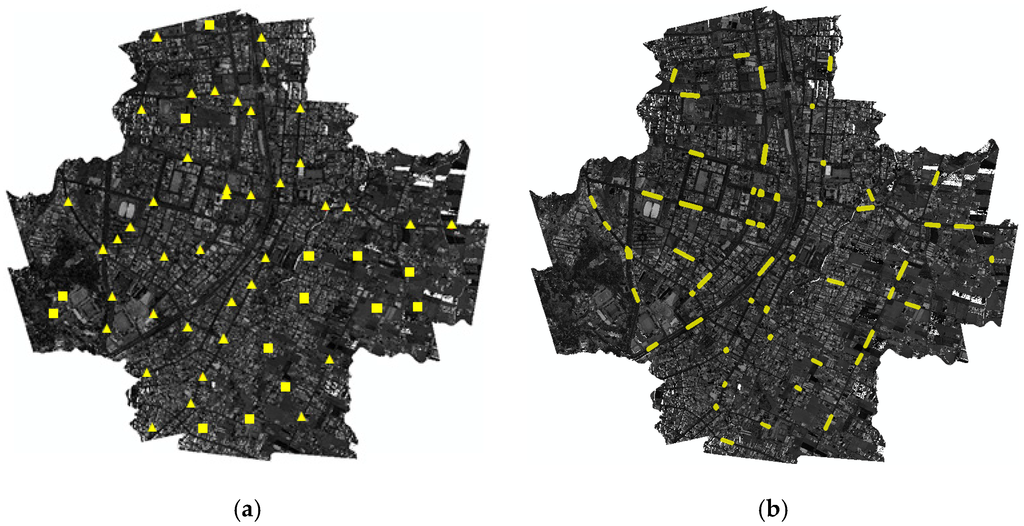
Figure 5.
The distribution of tie regions: (a) ground control regions (GCR) by automatic tie region selection, the triangles indicate road regions and squares indicates rooftop regions; and (b) independent check regions (ICR) by manual selection.
We applied both the backscattering coefficient and corrected intensity in multi-strip calibration for radiometric alignment. The concept of lidar radiometric normalization is to calculate the compensated parameters for each strip and reduce the difference between strips. At most ranges, incident angle and system effects are corrected via single-strip radiometric correction, and the remaining radiometric bias can be compensated by a linear function (i.e., gain and offset). The observation (measurement) was the control tie regions between strips, and these control tie regions were used to determine compensation parameters (Figure 6).
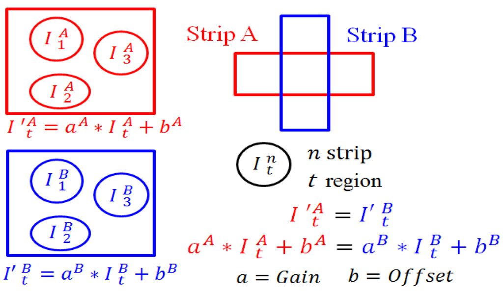
Figure 6.
Illustration of multi-strip adjustment for strips A and B.
Considering a multi-strip lidar dataset with number of strips, , where , each strip should be compensated by gain and offset parameters in radiometric block adjustment. The number of tie regions was and number of pairs between strips was . The average radiance of the tie region in strip is denoted as , where . The radiance can be compensated into by gain and offset parameters (Equation (7)):
Assuming that the tie region radiance in the overlapped area should be the same, the corrected radiances of the region from strip i and strip j satisfied Equation (8), assuming that a set of observation equations from all strips was F, , where . The observation equation was defined as Equation (9) in which pairs of tie regions establish observation equations from all strips. Equation (9) was substituted by Equation (7) to form Equation (10), in which the measurement was the average radiance from the tie region, and unknown parameters were gain and offset .
For M pairs of tie regions, the observation equation is represented in matrix form as Equations (11)–(13). Matrix A comprised homogeneous linear equations and X non-zero unknown parameters. To solve for these linear equations, we used singular value decomposition (SVD) [38]. These linear equations were independent, and the rank of matrix A was larger than the number of unknown parameters. More notably, they were required to maintain a restraint condition of compensatory parameters for the model to remain physically plausible. As discussed earlier, and were assumed to be different for each strip but stabilized around theoretical values (e.g., , ).
3.4. Accuracy Assessment
The aim of radiometric block adjustment is to reduce the radiometric difference between strips in overlapped regions. The accuracy analysis included quantitative and qualitative assessments. In quantitative analysis, the backscattered energy from different strips should have similar responses after block adjustment; therefore, we compared the differences in the overlapped area before and after adjustment. An improvement rate was also provided to analyze the performance of block adjustment (Equation (14)). In the qualitative analysis, we visually compared the results before and after radiometric block adjustment and used the radiometric profiles to evaluate the radiometric continuity between strips.
where is standard error before radiometric normalization; is standard error after radiometric normalization.
4. Results and Discussions
4.1. Quantitative Analyses
In order to evaluate the quality of parameter determination, we calculate the additional sigma naught (σ0) as an overall quality index. All the 54 tie regions are used in radiometric block adjustment. The σ0 for backscattering coefficient and intensity block adjustment are 0.0047 and 0.0039, respectively. As the numerical ranges for backscattering coefficient and intensity is 0 to 1 in radiometric block adjustment, the σ0 is relatively a very small value. We also calculate the variation of coefficients in radiometric block adjustment. The uncertain of coefficients are very small too; they are less than 0.030 for backscattering coefficient and 0.043 for corrected intensity. The sigma naught and variation of coefficients indicated that the parameter determination in block adjustment is stable and reliable.
The quantitative results included the variance of difference and improvement rate from control and check tie regions. We compared the results of radiometric block adjustment using backscattering coefficient (γ) and corrected intensity (I) (Table 2). For the check tie region, the standard deviations of delta γ before and after radiometric block adjustment were 0.112 and 0.041, respectively, and the standard deviations of delta I before and after radiometric block adjustment were 38.53 and 10.14, respectively, both of which showed significant improvement after block adjustment. The results indicated that the improvement of radiometric consistency reached about 63.5% to 73.6% for check tie regions.
To compare the backscattering coefficient and corrected intensity, the backscattering coefficient was normalized by several waveform parameters (Equation (3)), whereas corrected intensity only considered range and incident angles (Equation (6)). The distribution of the corrected intensity was larger than the backscattering coefficient before block adjustment; therefore, delta I was larger than delta γ before correction. The numerical result indicated that the discrete lidar may adopt intensity, whereas waveform lidar may use backscattering coefficient in radiometric block adjustment. The backscattering coefficient and corrected intensity can be used in radiometric normalization respectively.

Table 2.
Improvement rates of the proposed methods.
| Residuals () | Single-Strip Adjustment | Multi-Strip Adjustment | Improvement | |||
|---|---|---|---|---|---|---|
| Mean | Std | Mean | Std | |||
| Backscattering coefficient (γ) | GCR | 0.158 | 0.213 | 0.038 | 0.056 | 73.78% |
| ICR | 0.127 | 0.112 | 0.038 | 0.041 | 63.58% | |
| Corrected intensity (I) | GCR | 42.75 | 37.98 | 6.02 | 9.02 | 76.23% |
| ICR | 42.17 | 38.53 | 6.86 | 10.14 | 73.68% | |
In order to evaluate the radiometric normalization using different materials, we compare the results of all regions, road regions and non-road regions using the same independent check regions (Table 3). The numbers of ground control region for all regions, road regions and non-road regions are 54, 40 and 14. All ground control regions (GCR) are automatically selected by the proposed method. The independent check regions are manually selected and the total number is 52. For the standard deviations of independent check regions (ICR) after multi-strip adjustment, the standard deviations of road region (i.e., 0.035) is smaller than non-road region (i.e., 0.052) as the road regions has lower reflectance than others. Therefore, the improvement rate from road regions is better than non-road regions. Overall, all the improvement rates have reached over 50% and the road and non-road regions are able to improve the consistency between strips.

Table 3.
Comparison of different materials in multi-strip adjustment.
| Residuals () | N | Single-Strip Adjustment | Multi-Strip Adjustment | Improvement | ||||
|---|---|---|---|---|---|---|---|---|
| Mean | Std | Mean | Std | |||||
| Backscattering coefficient (γ) | All | GCR | 54 | 0.158 | 0.213 | 0.038 | 0.056 | 73.78% |
| ICR | 52 | 0.127 | 0.112 | 0.038 | 0.041 | 63.58% | ||
| Road | GCR | 40 | 0.140 | 0.161 | 0.029 | 0.047 | 70.61% | |
| ICR | 52 | 0.127 | 0.112 | 0.028 | 0.035 | 69.01% | ||
| Non-Road | GCR | 14 | 0.243 | 0.366 | 0.087 | 0.082 | 77.66% | |
| ICR | 52 | 0.127 | 0.112 | 0.081 | 0.052 | 53.43% | ||
| Corrected intensity (I) | All | GCR | 54 | 42.75 | 37.98 | 6.02 | 9.02 | 76.23% |
| ICR | 52 | 42.17 | 38.53 | 6.86 | 10.14 | 73.68% | ||
| Road | GCR | 40 | 41.24 | 33.43 | 4.64 | 7.43 | 77.76% | |
| ICR | 52 | 42.17 | 38.53 | 5.65 | 9.54 | 75.23% | ||
| Non-Road | GCR | 14 | 50.06 | 54.97 | 13.15 | 12.28 | 77.65% | |
| ICR | 52 | 42.17 | 38.53 | 19.77 | 16.53 | 57.11% | ||
Lin [39] indicated that flying height (range) was one of the important factors for amplitude/intensity. To investigate the effect of range and intensity/backscattering coefficient, the delta intensity (dI) and delta backscattering coefficient (dγ) of tie regions were also provided (Figure 7) to compare the results of single- and multi-strip adjustments at different delta ranges (dR) from ICR. In Figure 7a, the squares indicate corrected intensities after single-strip adjustment while the triangles show normalized intensities after multi-strip adjustment for ICR. The y-axis is delta intensity (dI) of ICR while the x-axis is delta slant range (dR) of ICR between overlapped strips. The variation of dI in single-strip adjustment (i.e., distribution of squares in y-direction) was larger than the results after multi-strip adjustment (i.e., distribution of triangles in y-direction). The dI was proportional to the dR and the linear regression of dI and dR was also provided in the figure. The slope of linear regression for multi-strip adjustment was smaller than slope of linear regression for single-strip adjustment. It means that the variation of dI was reduced significantly and the intensities between strips were more consistency after multi-strip adjustment. The behavior of delta backscattering coefficient (Figure 7b) was similar to delta intensity (Figure 7a). In addition, the influence of dR for dI was larger than dγ because the backscattering coefficient considers more parameters than the corrected intensity. Figure 7c,d shows the relationship between delta incident angle and dI / dγ. The variations of dI and dγ were become smaller after multi-strip adjustment.
The multi-strip radiometric adjustment includes two strategies: pair-wise adjustment [32] and block adjustment. The pair-wise adjustment considers the radiometrical balancing between two strips. Every slave strip is referred to a master strip separately using pair-wise adjustment. The block adjustment considers the radiometrical balancing globally for all available strips in the least squares sense. Besides, the pair-wise adjustment used histograms, while the proposed method used the homogeneous control regions in an overlapped area. The proposed method is a block adjustment process to minimize globally the radiometrical discrepancies for all strips. Table 4 shows the comparison of the proposed method and the pair-wise adjustment using piece-wise histogram matching [32]. Both methods use the same check regions to evaluate the consistency of intensities and backscattering coefficients between strips. The experimental results indicate that the means of delta γ and delta I for block adjustment are smaller than pair-wise adjustment. The test area contains nine strips; therefore, block adjustment is more suitable for data set with cross-over strips.
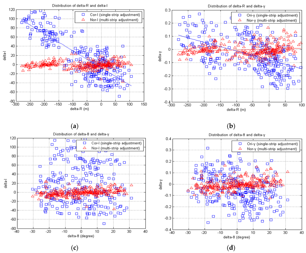
Figure 7.
Distributions of delta intensity and delta backscattering coefficient: (a) the distributions of delta intensity and delta slant range; (b) the distributions of delta backscattering coefficient and delta slant range; (c) the distributions of delta intensity and delta incident angle; and (d) the distributions of delta backscattering coefficient and delta incident angle.

Table 4.
Comparison of block and pair-wise adjustments.
| Before | After | Improvement | |||||
|---|---|---|---|---|---|---|---|
| Mean | Std. | Mean | Std. | ||||
| Backscattering Coefficient (γ) | Block Adjustment | ICR | 0.127 | 0.112 | 0.038 | 0.041 | 63.58% |
| Pair-Wise Adjustment | ICR | 0.127 | 0.112 | 0.110 | 0.067 | 40.07% | |
| Corrected Intensity (I) | Block Adjustment | ICR | 42.17 | 38.53 | 6.86 | 10.14 | 73.68% |
| Pair-Wise Adjustment | ICR | 42.17 | 38.53 | 16.82 | 17.99 | 53.29% | |
4.2. Qualitative Analysis
In qualitative analysis, multi-strip lidars were mosaicked to obtain a wider coverage (Figure 8). We used average of pixel values from different strips to generate mosaicked image. The result of single-strip adjustment was first corrected from the physically-oriented model, then the biases were minimized through block adjustment by the data-oriented model. The result of multi-strip adjustment showed higher consistency than the single-strip adjustment.
A comparison of results of the backscattering coefficient (Figure 8b) and intensity (Figure 8e) after single-strip adjustment showed that the radiometric consistency of the backscattering coefficient performed better than intensity because the single-strip adjustment of intensity only considered the range and angle effects. The pulse energy, beam size, and other effects were not applied in corrected intensity. A comparison of intensity before (Figure 8e) and after (Figure 8f) multi-strip adjustment showed that the results of block adjustment were more uniform than the single-strip adjustment.
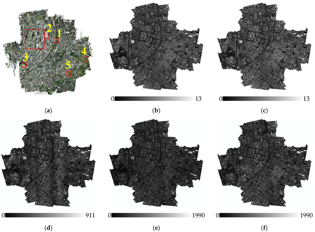
Figure 8.
Results of normalized intensity and backscattering coefficient: (a) optical image; (b) original backscattering coefficient; (c) normalized backscattering coefficient; (d) original intensity; (e) corrected intensity; and (f) normalized intensity.
To compare the mosaicked results from single- and multi-strip adjustments, five areas covering seam lines were enlarged (Figure 9). The results of single-strip adjustment showed inconsistencies near seam lines. After multi-strip adjustment, the results of normalized intensity showed higher consistency than the single-strip adjustment. Both intensity and backscattering coefficients improved near seam lines.
Qualitative analysis included two aspects: one to check the consistency in overlapped areas, and another to evaluate the continuity at seam lines. In the continuity check, we manually selected five profiles (Figure 8a) at seam lines located in amplitude and echo width were also extracted from the Gaussian function (e.g., road, grass, concrete) and used them to check the radiometric continuity between strips. Theoretically, the return energy of planar areas should be stable after strip adjustment. The profiles of strip adjustment had larger undulations than block adjustment, but after block adjustment, the discontinuity between strips was reduced (Figure 9). In the consistency check, we selected an overlapped area (Figure 8a) containing different land cover types. Whether using the backscattering coefficient or corrected intensity, the differences were significantly improved and overall differences were decreased (Figure 10 and Figure 11). According to the radiometric differences between strips, the delta I of block adjustment was lower than the single adjustment, especially in flat areas. Delta γ behaved similarly, indicating that the difference between strips was reduced after block adjustment.
The largest differences occurred at the boundaries of trees and buildings. It is caused by penetration at near-edge area. There is no big difference in non-edge area. We have provided the histograms of delta I and delta γ in Figure 12. The histograms of delta I after multi-strip adjustment is more centralize to zero than the histogram of single-strip adjustment. Beside the distribution of delta I after multi-strip adjustment is also smaller than delta I in single-strip adjustment. The histograms of delta γ show the similar behavior like delta intensity.
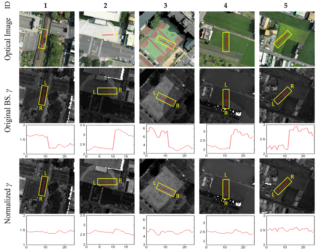
Figure 9.
Profiles of check regions.
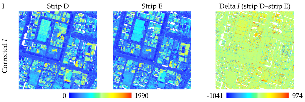

Figure 10.
Delta intensity in overlapped area.
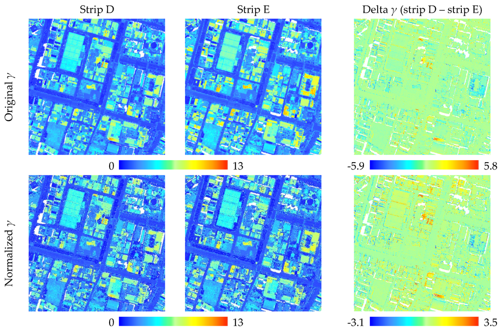
Figure 11.
Delta backscattering coefficient in overlapped area.
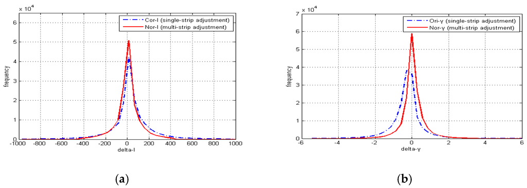
Figure 12.
Histogram of delta intensity and delta backscattering coefficient in overlapped area: (a) delta intensity before and after multi-strip normalization; and (b) delta backscattering coefficient before and after normalization.
Figure 13 is the zoom-in view to demonstrate the intensities in two overlapped strips. Figure 13f,j shows the distributions of original, corrected (i.e., results of single-strip adjustment) and normalized (i.e., results of multi-strip adjustment) intensities for strips C and G. Figure 13k superimposes the corrected intensities of strips C and G. The corrected intensity of strip C is slightly larger than strip G. After multi-strip adjustment, the discrepancies can be compensated as shown as Figure 13.
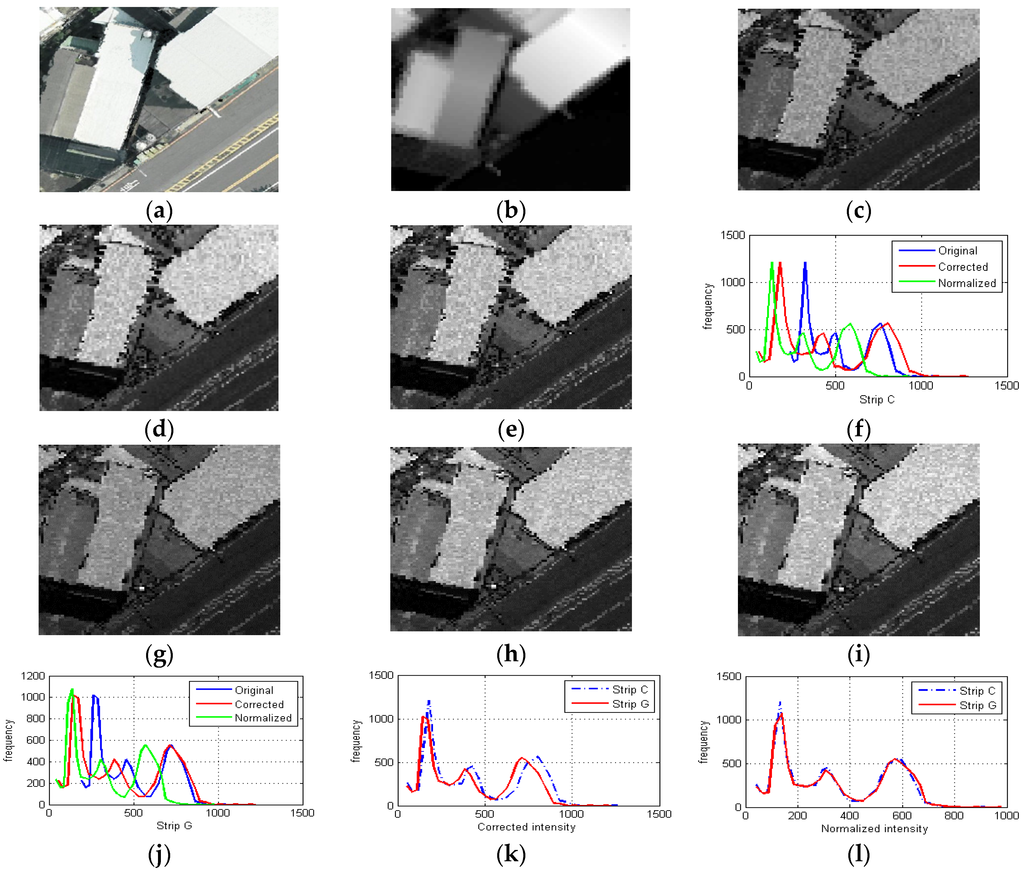
Figure 13.
Zoom-in overlapped area: (a) aerial photo; (b) DSM; (c) original intensity of strip C; (d) corrected intensity of strip C; (e) normalized intensity of strip C; (f) histograms of strip C; (g) original intensity of strip G; (h) corrected intensity of strip G; (i) normalized intensity of strip G; (j) histograms of strip G; (k) histograms of corrected intensity of strips C and G; and (l) histograms of normalized intensity of strips C and G.
5. Conclusion and Future Work
This study proposed a radiometric normalization model to improve the radiometric consistency between multi-strip lidars. A framework of radiometric block adjustment was developed to validate the proposed scheme. The advantage of the proposed method was utilizing reliable tie regions to reduce the radiometric discrepancy in overlapped regions. Moreover, this model was data-independent and can therefore be successfully applied to backscattering coefficient from waveform lidar and intensity from discrete lidar. The major contributions of this study were to (1) establish a radiometric normalization scheme for multi-strip lidars; (2) improve the radiometric consistency through model-driven single-strip adjustment and data-driven block adjustment; and (3) compare results of backscattering coefficient and corrected intensity in radiometric normalization.
The proposed scheme integrates model-driven single-strip adjustment and data-driven block adjustment in radiometric normalization, subsequently improving the radiometric consistency between multi-strip lidars. The conclusions are summarized as follows:
- (1)
- Systematic error can be eliminated through the radiometric block adjustment. Experimental results indicated that the proposed method may improve the radiometric consistency between multiple strips. The improvement rate for backscattering coefficient and corrected intensity reached 63% and 73% in overlapped area.
- (2)
- In model-driven single-strip adjustment, the consistency of backscattering coefficient was better than intensity. After the data-driven block adjustment, both the backscattering coefficient and intensity showed similar results.
- (3)
- In the qualitative check, the backscattering coefficient and corrected intensity became more consistent after normalization in overlapped areas. Profiles at seam lines also showed high continuity after normalization.
- (4)
- In the mosaicking of multi-strip lidars, the mosaicked data removed the inconsistency and can be used in land cover recognition, classification, and other applications.
In this study, the proposed method used multiple flight lines from single wavelength airborne lidar system. As the development of multi-wavelength lidar system [14], future work will evaluate the suitability of multiple flight lines adjustment from different wavelengths. Besides, the future work will also extend the radiometric block adjustment for the needs of multi-stations terrestrial lidar system [17].
Acknowledgments
This research was partially supported by the Ministry of Science and Technology of Taiwan under project number NSC 101-2628-E-009-019-MY3. The authors would like to thank Strong Engineering Consulting Co., Ltd in Taiwan for providing the test datasets.
Author Contributions
Tee-Ann Teo provided the overall conception of this research, designed the methodologies and experiments, and wrote the majority of the manuscript. Hsien-Ming Wu contributed to the implementation of proposed algorithms, conducted the experiments and performed the data analyses.
Conflicts of Interest
The authors declare no conflict of interest.
References
- Shan, J.; Sampath, A. Urban DEM generation from raw lidar data: A labeling algorithm and its performance. ISPRS J. Photogramm. Remote Sens. 2005, 71, 217–226. [Google Scholar] [CrossRef]
- Kaasalainen, S.; Krooks, A.; Kukko, A.; Kaartinen, H. Radiometric calibration of terrestrial laser scanners with external reference targets. Remote Sens. 2009, 1, 144–158. [Google Scholar] [CrossRef]
- Vosselman, G.; Kessels, P.; Gorte, B. The utilisation of airborne laser scanning for mapping. Int. J. Appl. Earth Obs. Geoinform. 2005, 6, 177–186. [Google Scholar] [CrossRef]
- Elberink, S.O.; Vosselman, G. Building reconstruction by target based graph matching on incomplete laser data: Analysis and limitations. Sensors 2009, 9, 6101–6118. [Google Scholar] [CrossRef] [PubMed]
- Sithole, G.; Vosselman, G. Bridge detection in airborne laser scanner data. ISPRS J. Photogramm. Remote Sens. 2006, 61, 33–46. [Google Scholar] [CrossRef]
- Tseng, Y.H.; Wang, C.K.; Chu, H.J.; Hung, Y.C. Waveform-based point cloud classification in land-cover identification. Int. J. Appl. Earth Obs. Geoinfor. 2015, 34, 78–88. [Google Scholar] [CrossRef]
- Kim, K.; Shan, J. Building roof modeling from airborne laser scanning data based on level set approach. ISPRS J. Photogramm. Remote Sens. 2011, 66, 484–497. [Google Scholar] [CrossRef]
- Rebecca, O.C.; Gold, C.; Kidner, D. 3D city modelling from lidar data. Adv. 3D Geoinform. Syst. 2008. [Google Scholar] [CrossRef]
- Sun, S.; Salvaggio, C. Aerial 3D building detection and modeling from airborne lidar point clouds. IEEE J. Sel. Top. Appl. Earth Obs. Remote Sens. 2013, 6, 1440–1449. [Google Scholar] [CrossRef]
- Filin, S.; Vosselman, G. Adjustment of airborne laser altimetry strips. Int. Arch. Photogramm. Remote Sens. Spat. Inform. Sci. 2004, 35, 285–289. [Google Scholar]
- Kager, H. Discrepancies between overlapping laser scanner strips–simultaneous fitting of aerial laser scanner strips. Int. Arch. Photogram. Remote Sens. Spat. Inform. Sci. 2004, 35, 555–560. [Google Scholar]
- Lee, J.; Yu, K.; Kim, Y.; Habib, A.F. Adjustment of discrepancies between lidar data strips using linear features. IEEE Geosci. Remote Sens. Lett. 2007, 4, 475–479. [Google Scholar] [CrossRef]
- Doneus, M.; Miholjek, I.; Mandlburger, G.; Doneus, N.; Verhoeven, G.; Briese, C.; Pregesbauer, M. Airborne laser bathymetry for documentation of submerged archaeological sites in shallow water. ISPRS Int. Ann. Photogramm. Remote Sens. Spat. Inform. Sci. 2015, 1, 99–107. [Google Scholar] [CrossRef]
- Rees, V.E. The first multispectral airborne lidar sensor. GeoInformatics 2015, 18, 10. [Google Scholar]
- Sawamura, P.; Müller, D.; Hoff, R.M.; Hostetler, C.A.; Ferrare, R.A.; Hair, J.W.; Rogers, R.R.; Anderson, B.E.; Ziemba, L.D.; Beyersdorf, A.J.; et al. Aerosol optical and microphysical retrievals from a hybrid multiwavelength lidar data set—DISCOVER-AQ 2011. Atmos. Meas. Tech. 2014, 7, 3113–3157. [Google Scholar] [CrossRef]
- Suvorina, A.S.; Veselovskii, I.A.; Whiteman, D.N.; Korenskiy, M.Y. Profiling of the forest fire aerosol plume with multiwavelength Raman lidar. Int. Laser Opt. Conf. 2014. [Google Scholar] [CrossRef]
- Hartzell, P.; Glennie, C.; Biber, K.; Khan, S. Application of multispectral lidar to automated virtual outcrop geology. ISPRS J. Photogramm. Remote Sens. 2014, 88, 147–155. [Google Scholar] [CrossRef]
- Wagner, W. Radiometric calibration of small-footprint full-waveform airborne laser scanner measurements: Basic physical concepts. ISPRS J. Photogramm. Remote Sens. 2010, 65, 505–513. [Google Scholar] [CrossRef]
- Wagner, W.; Ullrich, A.; Ducic, V.; Melzer, T.; Studnicka, N. Gaussian decomposition and calibration of a novel small-footprint full-waveform digitising airborne laser scanner. ISPRS J. Photogramm. Remote Sens. 2006, 60, 100–112. [Google Scholar] [CrossRef]
- Abed, F.M.; Mills, J.P.; Miller, P.E. Echo amplitude normalization of full-waveform airborne laser scanning data based on robust incidence angle estimation. IEEE Trans. Geosci. Remote Sens. 2012, 50, 2910–2918. [Google Scholar] [CrossRef]
- Briese, C.; Höfle, B.; Lehner, H.; Wagner, W.; Pfennigbauer, M.; Ullrich, A. Calibration of full-waveform airborne laser scanning data for object classification. Conf. Laser Radar Technol. Appl. 2008. [Google Scholar] [CrossRef]
- Kaasalainen, S.; Hyyppä, J.; Litkey, P.; Hyyppä, H.; Ahokas, E.; Kukko, A.; Kaartinen, H. Radiometric calibration of ALS intensity. Int. Arch. Photogramm. Remote Sens. Spat. Inf. Sci. 2007, 36, 201–205. [Google Scholar]
- Roncat, A.; Bergauer, G.; Pfeifer, N. B-spline deconvolution for differential target cross-section determination in full-waveform laser scanning data. ISPRS J. Photogramm. Remote Sens. 2011, 66, 418–428. [Google Scholar] [CrossRef]
- Ding, Q.; Chen, W.; King, B.; Liu, Y.; Liu, G. Combination of overlap-driven adjustment and Phong model for lidar intensity correction. ISPRS J. Photogramm. Remote Sens. 2013, 75, 40–47. [Google Scholar] [CrossRef]
- Phong, B.T. Illumination for computer generated pictures. Commun. ACM 1975, 18, 311–317. [Google Scholar] [CrossRef]
- Höfle, B.; Hollaus, M.; Hagenauer, J. Urban vegetation detection using radiometrically calibrated small-footprint full-waveform airborne lidar data. ISPRS J. Photogramm. Remote Sens. 2012, 67, 137–147. [Google Scholar] [CrossRef]
- Höfle, B.; Pfeifer, N. Correction of laser scanning intensity data: Data and model-driven approaches. ISPRS J. Photogramm. Remote Sens. 2007, 62, 415–433. [Google Scholar] [CrossRef]
- Jutzi, B.; Gross, H. Normalization of lidar intensity data based on range and surface incidence angle. Int. Arch. Photogramm. Remote Sens. Spat. Inf. Sci. 2009, 38, 213–218. [Google Scholar]
- Alexander, C.; Tansey, K.; Kaduk, J.; Holland, D.; Tate, N.J. Backscatter coefficient as an attribute for the classification of full-waveform airborne laser scanning data in urban areas. ISPRS J. Photogramm. Remote Sens. 2010, 65, 423–432. [Google Scholar] [CrossRef]
- Chandelier, L.; Martinoty, G. Radiometric aerial triangulation for the equalization of digital aerial images and orthoimages. Photogramm. Eng. Remote Sens. 2009, 75, 193–200. [Google Scholar] [CrossRef]
- Pros, A.; Colomina, I.; Navarro, J.A.; Antequera, R.; Andrinal, P. Radiometric block adjustment and digital radiometric model generation. Int. Arch. Photogramm. Remote Sens. Spat. Inf. Sci. 2013, XL-1/W1, 293–298. [Google Scholar] [CrossRef]
- Yan, W.Y.; Shaker, A. Radiometric correction and normalization of airborne lidar intensity data for improving land-cover classification. IEEE Trans. Geosci. Remote Sens. 2014, 52, 7658–7673. [Google Scholar]
- APSRS Las specification version 1.3-R10. Available online: http://www.asprs.org/a/society/committees/standards/asprs_las_spec_v13.pdf (accessed on 6 June 2015).
- RIEGL RiWorld User Manual. Available online: http://www.riegl.com/products/software-packages/riworld/ (accessed on 10 December 2015).
- Teo, T.A.; Huang, S.H. Surface-based registration of airborne and terrestrial mobile lidar point clouds. Remote Sens. 2014, 6, 12686–12707. [Google Scholar] [CrossRef]
- Kaasalainen, S.; Pyysalo, U.; Krooks, A.; Vain, A.; Kukko, A.; Hyyppä, J.; Kaasalainen, M. Absolutie radiometric calibration of ALS inteisyt data: Effects on accuracy and target classification. Sensors 2011, 11, 10586–10602. [Google Scholar] [CrossRef] [PubMed]
- Pauly, M.G.M.; Kobbelt, L.P. Efficient simplification of point-sampled surfaces. Proc. IEEE Vis. 2002, 2, 163–170. [Google Scholar]
- Willian, H.P.; Sual, A.T.; Willian, T.V.; Brian, P.F. Numerical Recipes in C; Cambridge University Press: Cambridge, UK, 1998. [Google Scholar]
- Lin, Y.C. Normalization of echo features derived from full-waveform airborne laser scanning data. Remote Sens. 2015, 7, 2731–2751. [Google Scholar] [CrossRef]
© 2015 by the authors; licensee MDPI, Basel, Switzerland. This article is an open access article distributed under the terms and conditions of the Creative Commons by Attribution (CC-BY) license (http://creativecommons.org/licenses/by/4.0/).