Article

Object-Based Canopy Gap Segmentation and Classification: Quantifying the Pros and Cons of Integrating Optical and LiDAR Data

1
Department of Geography, University of Toronto, 100 St. George Street, Toronto, ON M5S 3G3, Canada
2
Forest Research and Monitoring Section, Ontario Ministry of Natural Resources and Forestry, 1235 Queen Street East, Sault Ste Marie, ON, P6A 2E5, Canada
3
Faculty of Forestry, University of Toronto, 33 Willcocks Street, Toronto, ON M5S 3B3, Canada
4
Department of Geography, University of Toronto Mississauga, 3359 Mississauga Rd North, Mississauga, ON L5L 1C6, Canada
*
Author to whom correspondence should be addressed.
Remote Sens. 2015, 7(12), 15917-15932; https://doi.org/10.3390/rs71215811
Submission received: 5 October 2015 / Revised: 4 November 2015 / Accepted: 19 November 2015 / Published: 27 November 2015
(This article belongs to the Special Issue Remote Sensing of Vegetation Structure and Dynamics)

Abstract

:
Delineating canopy gaps and quantifying gap characteristics (e.g., size, shape, and dynamics) are essential for understanding regeneration dynamics and understory species diversity in structurally complex forests. Both high spatial resolution optical and light detection and ranging (LiDAR) remote sensing data have been used to identify canopy gaps through object-based image analysis, but few studies have quantified the pros and cons of integrating optical and LiDAR for image segmentation and classification. In this study, we investigate whether the synergistic use of optical and LiDAR data improves segmentation quality and classification accuracy. The segmentation results indicate that the LiDAR-based segmentation best delineates canopy gaps, compared to segmentation with optical data alone, and even the integration of optical and LiDAR data. In contrast, the synergistic use of two datasets provides higher classification accuracy than the independent use of optical or LiDAR (overall accuracy of 80.28% ± 6.16% vs. 68.54% ± 9.03% and 64.51% ± 11.32%, separately). High correlations between segmentation quality and object-based classification accuracy indicate that classification accuracy is largely dependent on segmentation quality in the selected experimental area. The outcome of this study provides valuable insights of the usefulness of data integration into segmentation and classification not only for canopy gap identification but also for many other object-based applications.

Graphical Abstract

1. Introduction

A canopy gap is defined as a small opening within a continuous and relatively mature canopy, where trees are absent (i.e., non-forest gaps) or much smaller than their immediate neighbors (i.e., forest gaps) [1]. Canopy gaps are usually formed from natural disturbances, such as individual tree mortality events caused by insect, disease [2], or silvicultural thinning or harvesting activities [3]. Canopy gaps play an important role in forest regeneration, turnover, and overall dynamics of forest ecosystems [1]. In northern hardwood forests, for example, the size of gaps plays a critical role in controlling the regeneration of tree species that are not tolerant of deep shade [4]. Canopy gaps can also lead to the transformation of understory microenvironments (e.g., solar energy, water, and nutrients), responsible for understory biodiversity and habitats. In boreal mixedwood forests, Vepakomma et al. [5] found that canopy gaps increased availability of abiotic resources within canopy gaps as well as up to 30 m into the surrounding forest.
Compared to manual interpretation, which requires extensive field validation and training, remote sensing offers an efficient and accurate alternative for automated canopy gap identification. Medium spatial resolution Landsat images were able to detect relatively large forest canopy gaps [6,7] but failed to map fine-scale canopy gaps (i.e., under 30 m in size) [8]. The emergence of high spatial resolution images accompanied with the prevalence of Object-Based Image Analysis (OBIA) have overcome this shortcoming. OBIA views a group of similar image pixels as a segment and is particularly useful for high spatial resolution image processing because geo-objects tend to occupy many pixels at a fine scale. Compared to the traditional pixel-based methods, OBIA reduces spectral variability within geo-objects and suppresses the “salt and pepper” noise in the classification map [9]. For example, Jackson et al. [10] evaluated the potential of high spatial resolution IKONOS image (4 m) for identifying windthrown gaps, and found it could characterize more gaps than manual interpretation of temporally coincident aerial photographs. In addition, He et al. [11] successfully separated non-vegetated trails, roads, and cut blocks from vegetated areas using high spatial resolution SPOT image. Malahlela, Cho and Mutanga [12] tested the utility of WorldView-2 image with eight spectral bands to delineate forest canopy gaps, and concluded that it yielded a higher accuracy than conventional images with four spectral bands. These studies demonstrate that broad-band multispectral images produced promising results for canopy gap identification. However, the saturation of visible-near-infrared [1] signals makes it a challenge to discriminate between tree canopies and forest gaps [12]. Narrow-band hyperspectral images could solve this problem but their prohibitive acquisition cost limits the exploitation of their full potential [13,14]. Light detection and ranging (LiDAR) data have recently become one of the most important data sources for analyzing canopy gap dynamics. Vepakomma et al. [15] used a LiDAR derived Canopy Height Model (CHM) to identify canopy gaps larger than 5 m2 in a conifer dominated forest. Gaulton and Malthus [16] compared CHM and point cloud based techniques, and observed that the latter resulted in a higher overall accuracy over CHM-based methods. Nevertheless, very few studies involving canopy gap delineation and classification have integrated passive multispectral images and active LiDAR data by taking advantage of both spectral and vertical information.
In our study, a synergistic use of optical and LiDAR data is adopted for canopy gap delineation and classification for a structurally complex forest, located in Haliburton Forest and Wildlife Reserve, Ontario, Canada. In the workflow of OBIA, canopy gap delineation refers to sketching the boundaries of canopy gaps, whereas object-based classification is adopted to categorize the delineated geo-objects into different types of canopy gaps including non-forest (2–6 m in height) and forest gaps (6–10 m in height). Canopy gap delineation is done through image segmentation, which is the prerequisite step for object-based classification. This study focuses on answering the following three research questions: (1) how does the synergistic use of optical and LiDAR data influence the quality of canopy gap segmentation; (2) what are the advantages of the synergistic use of optical and LiDAR data in the process of object-based canopy gap classification; and (3) to what extent can the quality of canopy gap segmentation affect the accuracy of object-based gap classification?

2. Methodology

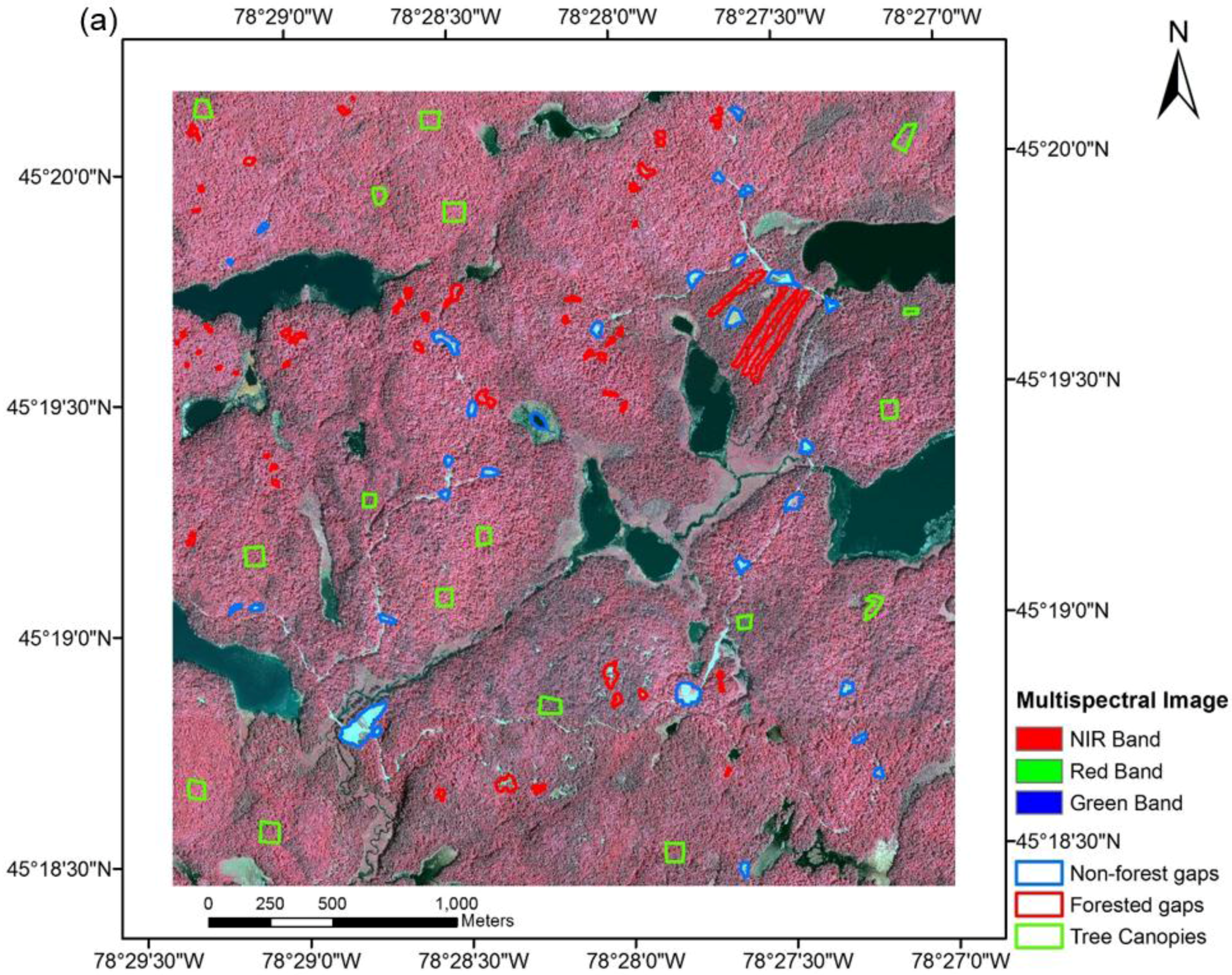
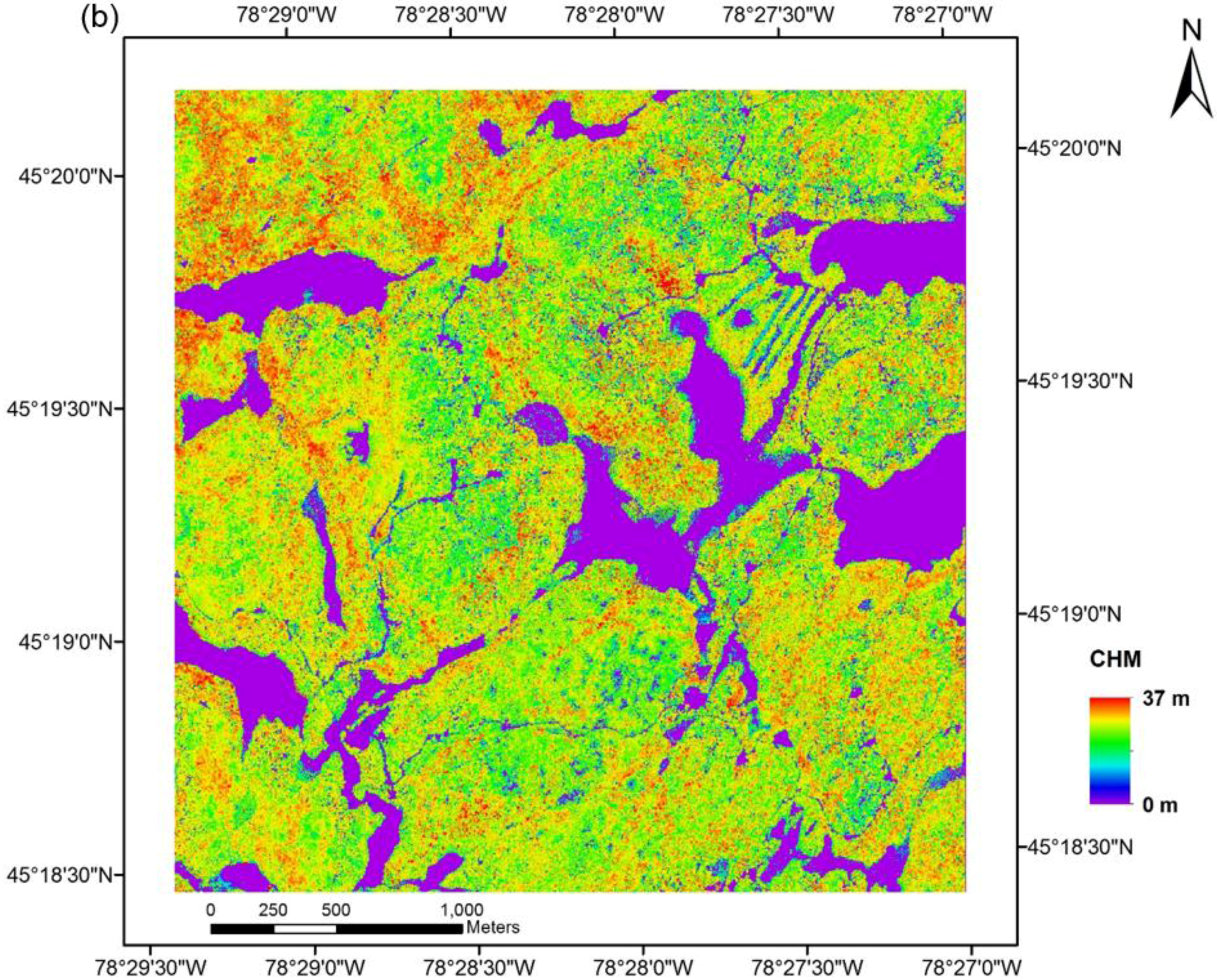
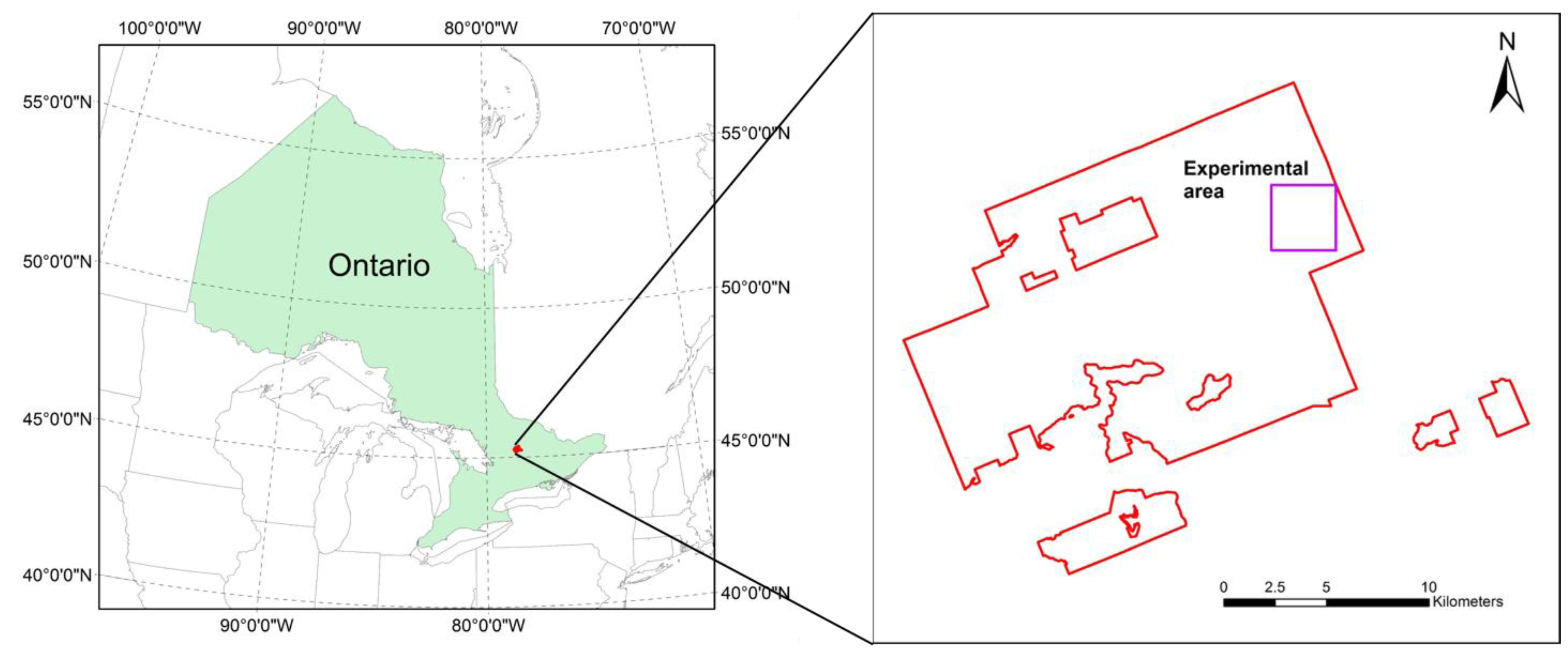
2.1. Study Area and Experimental Site Selection

Our study was carried out in Haliburton Forest and Wildlife Reserve, located in the Great Lakes-St. Lawrence region of central Ontario, Canada (Figure 1). The forest is approximately 30,000 ha in area and is primarily composed of uneven-aged, mixed-deciduous forest dominated by shade-tolerant hardwood species. At present, sugar maple (Acer saccharum) represents approximately 60% of basal area with American beech (Fagus grandifolia), yellow birch (Betula alleghaniensis), black cherry (Prunus serotina), balsam fir (Abies balsamea), and eastern hemlock (Tsuga canadensis) also present and relatively abundant [17].
Figure 1. Location of the experimental site in Haliburton Forest and Wildlife Reserve, Ontario, Canada.
Remotesensing 07 15811 g001
The experimental site (approximately 1000 hectares) was chosen for the study (Figure 1) because canopy gaps vary in type, size, and structure (water bodies included) in this site.

2.2. Multi-Source Remote Sensing Data
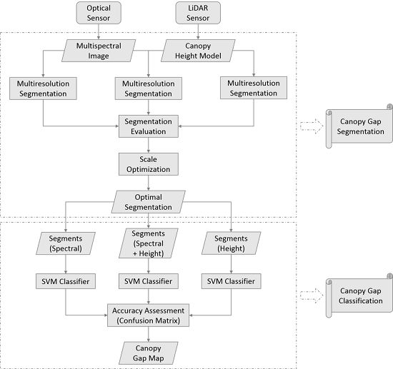
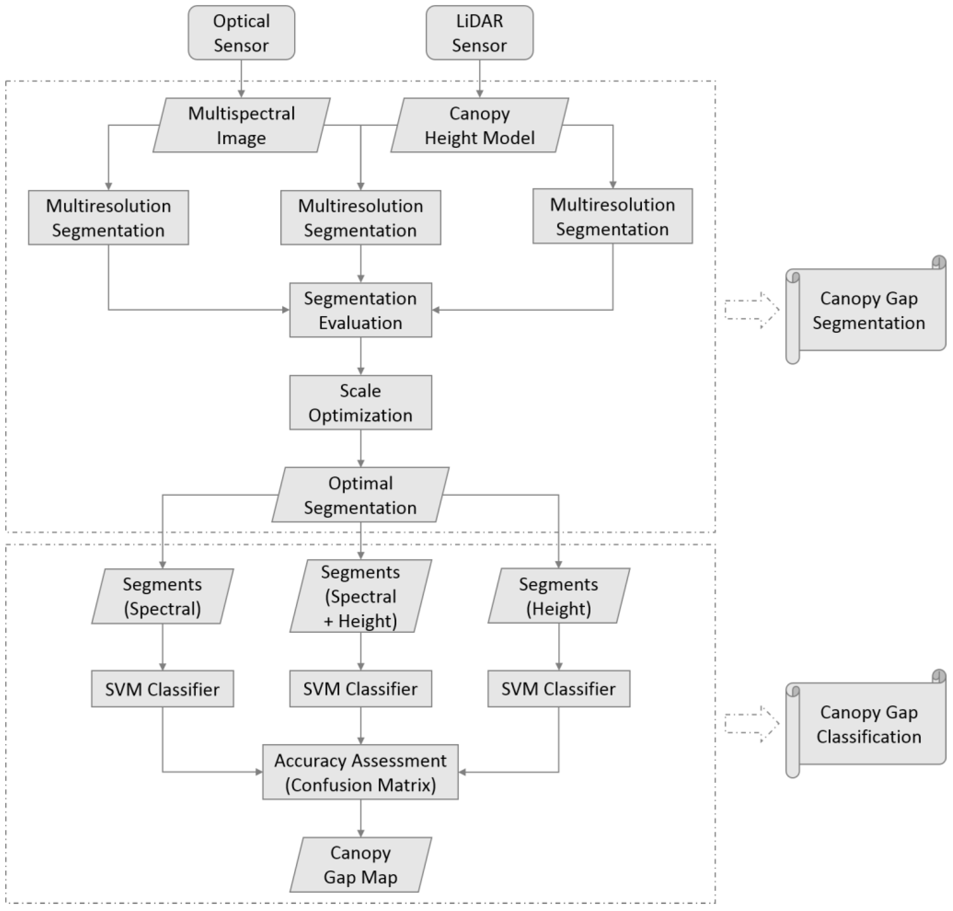
The optical multispectral image was acquired using the ADS40 airborne sensor by the Ontario Ministry of Natural Resources and Forestry (OMNRF) in the summer of 2007. The image contains four spectral bands (i.e., blue: 420–492 nm, green: 533–587 nm, red: 604–664 nm, near infrared (NIR): 833–920 nm) with a spatial resolution of 0.4 m. LiDAR data were collected by an Optech Airborne Laser Terrain Mapper (ALTM) 3100 LiDAR system in the summer of 2009. The flight was conducted at a height of 1500 m with a 16-degree field of view, a scan rate of 36 Hz, and a maximum pulse repetition frequency of 70 kHz. The average sampling point density is 1.7 points per square meter. In the process of creating the CHM, the LiDAR points within the study area were normalized to the terrain and outliers were filtered. The height of each pixel (cell size: 2 m) was derived by the maximum normalized LiDAR point that intersected the 2 m pixel (Haliburton & Nipissing LiDAR Survey). The multispectral image and CHM were clipped to cover the whole experimental site (Figure 2). As the CHM derived from the LiDAR data had a spatial resolution of 2.0 m, the multispectral image was further resampled to the spatial resolution of 2.0 m by the nearest neighbor method to keep the data compatible.
Figure 2. Multispectral image (a) and LiDAR derived CHM (b) for the experimental site (under the NAD83 UTM coordinate system). Blue, red, and green polygons represent the reference non-forest gaps (2–6 m in height), forest gaps (6–10 m in height), and tree canopies, respectively.
Remotesensing 07 15811 g002aRemotesensing 07 15811 g002b

2.3. Methods

The processing steps for the automated canopy gap delineation and classification are shown in Figure 3. Image segmentation was implemented to delineate canopy gaps at a range of scale parameters over three data sources: (1) the multispectral image; (2) the CHM; and (3) the combination of multispectral image and CHM. The suitable scale parameter that produced the best segmentation was identified and the best segmentation map from three data sources was then adopted for subsequent object-based classifications. Next, the geo-objects in the best segmentation were assigned with spectral (multispectral image), height (CHM), or both of spectral and height information for classification, and were further automatically categorized into three classes: non-forest gaps, forest gaps, and tree canopies. The classification accuracies were quantified by the parameters derived from the confusion matrices. The relation between the segmentation quality and the classification accuracy was investigated at the end.
Figure 3. The flowchart of the automated gap delineation and classification using optical and LiDAR data.
Remotesensing 07 15811 g003

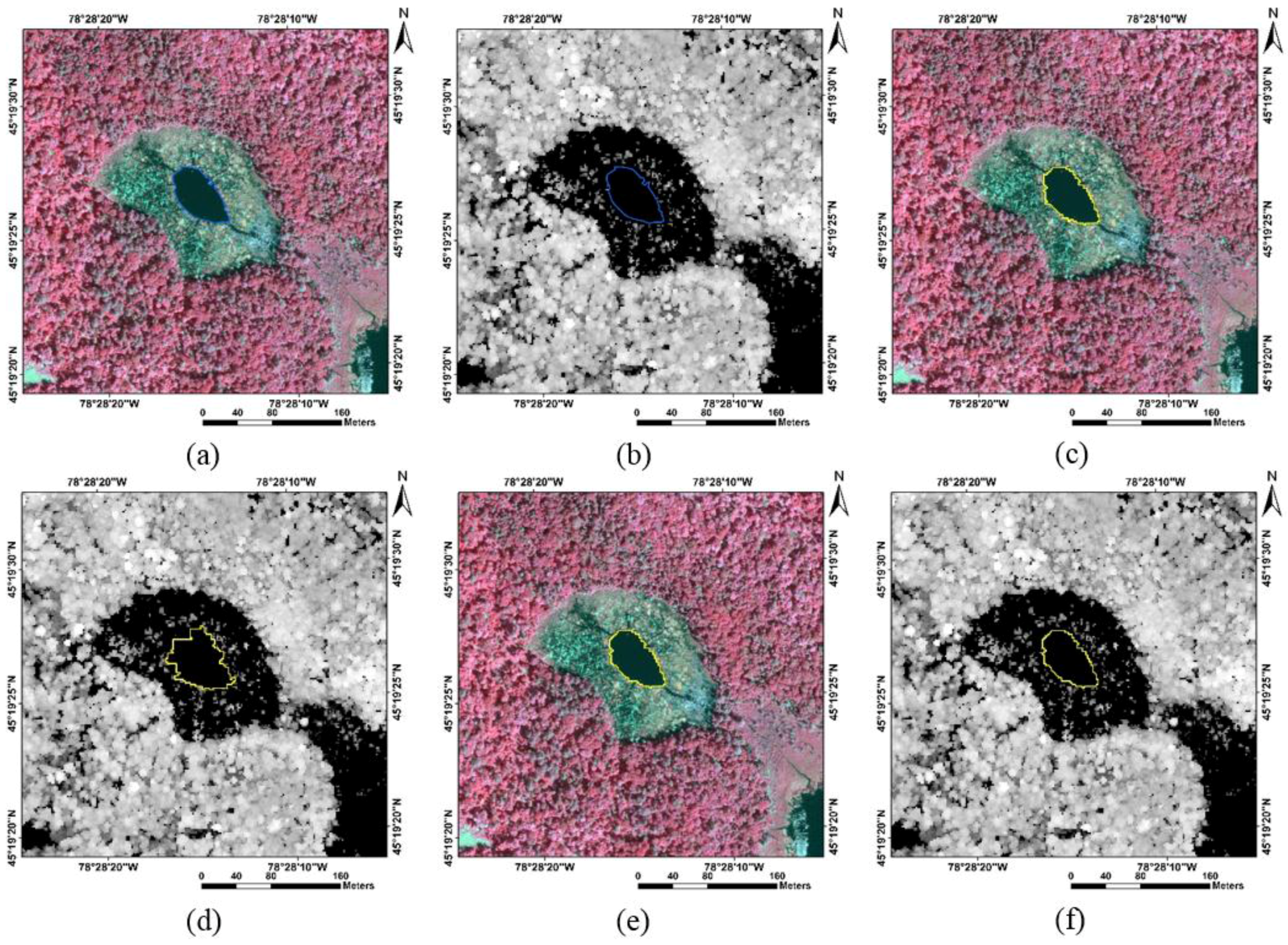
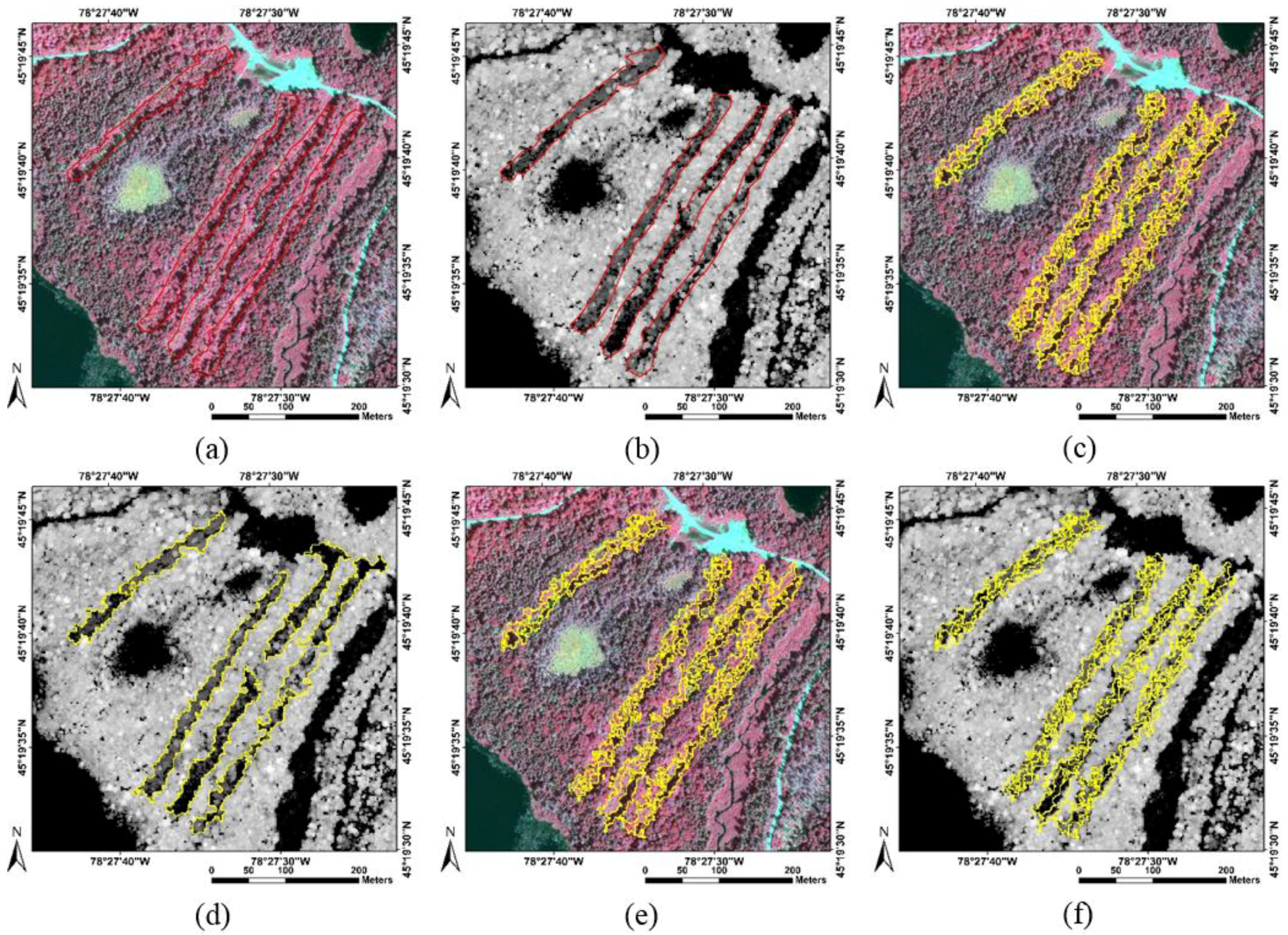
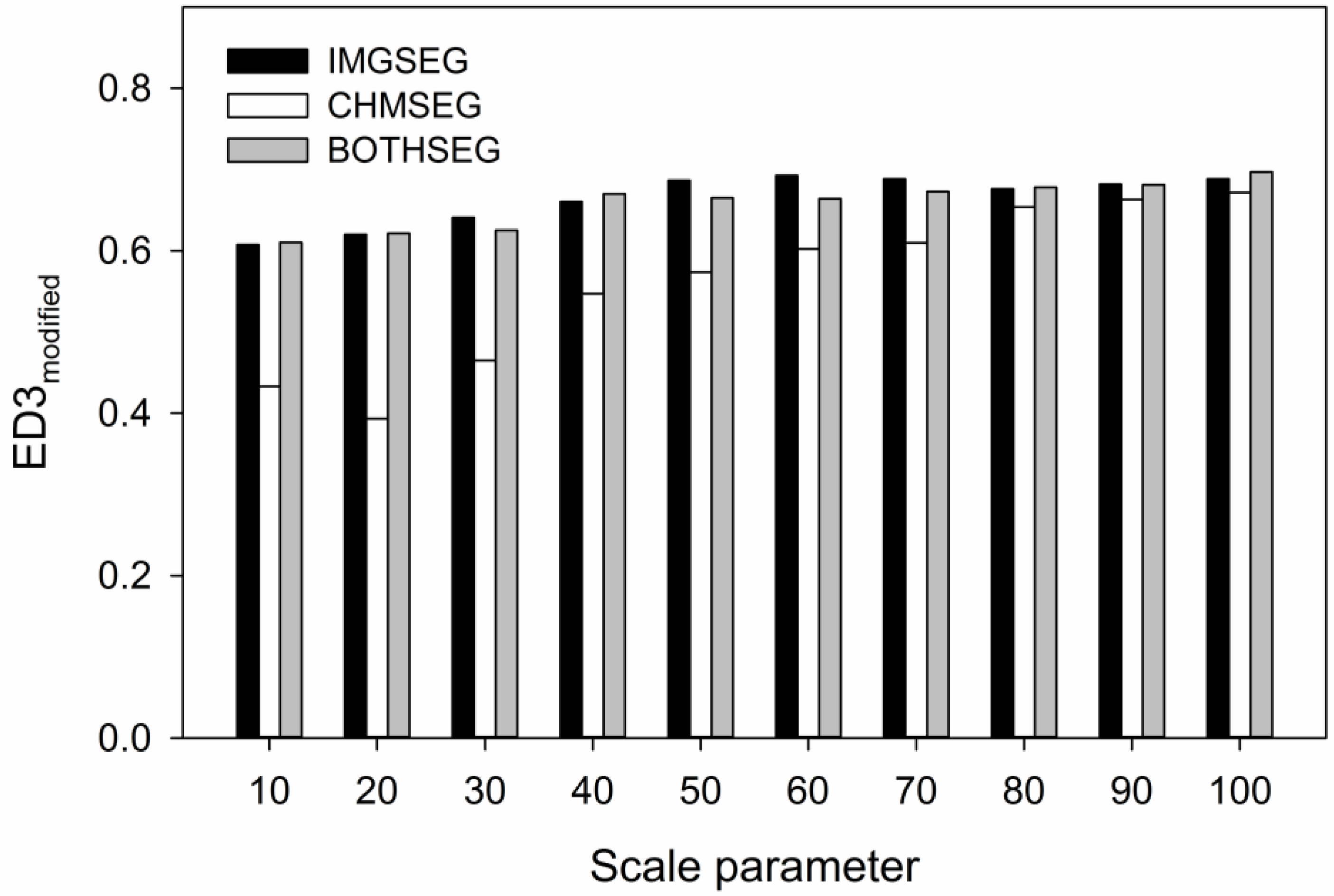
2.3.1. Canopy Gap Delineation

To segment canopy gaps, we employed a prevailing segmentation algorithm (i.e., multiresolution segmentation (MRS)) implemented in the Trimble eCognition Developer software package. MRS uses a local-oriented region merging technique that executes pairwise merging within a local vicinity [18]. The segmentation process is controlled by three parameters—scale, shape, and compactness [19]—and the size of segments is primarily determined by the scale parameter. In general, a high scale parameter produces larger segments whereas a low scale parameter produces smaller segments. In our experiment, the scale parameter was adjusted to produce different segmentation results while the other two parameters (i.e., shape and compactness) were fixed as the default values (i.e., 0.1 and 0.5) because canopy gaps varied in shape and compactness. When more than one data source was used in the MRS process, each layer was weighted equally.
Canopy gap delineation was achieved through image segmentation, so the accuracy of canopy gap delineation can be assessed by segmentation evaluation algorithms. Of many existing measures of segmentation evaluation (e.g., analytical and empirical goodness), the indicators of empirical discrepancy have been demonstrated to be most effective [20,21] because they capture the dissimilarity between a reference polygon and a corresponding segment. In recent years, many discrepancy measures have been proposed [22,23,24,25]. Yang et al. [26] proposed the indicator of Modified Euclidean Distance 3 (ED3Modified) in order to measure local metrics of geometric and arithmetic discrepancy and globalize the ED3Modified with equal weight to each reference polygon over the whole image. The ED3Modified value ranges from 0 to 0.71 with a lower value indicating a better segmentation. Yang et al. [27] later developed a new discrepancy measure, Segmentation Evaluation Index (SEI), to quantify the segmentation accuracy from the perspective of geo-object recognition. The SEI indicator is a more strict discrepancy measure because it requires a one-to-one correspondence between reference polygons and candidate segments. Similar to the modified ED3, a lower value of SEI indicates a higher quality of segmentation, although SEI ranges from 0 to 1. Since SEI is a more strict indicator of over-segmentation than ED3Modified [26,27] and since over-segmented geo-objects does not impact the object-based classification as negatively as under-segmented geo-objects, we decided to use ED3Modified to quantify the accuracy of canopy gap delineation at scale parameters between 10 and 100. We manually digitized 29 reference polygons for non-forest and 53 reference for forest gaps (Figure 2). A total of 82 reference polygons were used to calculate the ED3Modified values to determine the quality of canopy gap segmentation. For the segmentation results at those scale parameters, one-way analysis of variance (ANOVA) was implemented to identify whether the synergistic use of optical and LiDAR data could significantly improve the accuracies of canopy gap segmentation. The best segmentation result was determined by the lowest value of ED3Modified, and was further used for the object-based canopy gap classification. We also calculated the SEI values for the above segmentation results in order to determine which index (i.e., ED3Modified or SEI) was more related to object-based classification accuracy.

2.3.2. Object-Based Canopy Gap Classification

The segmented geo-objects were assigned with spectral, height, or both of spectral and height information (i.e., the mean pixel values within the segments) and then classified into three classes: non-forest gaps, forest gaps, and tree canopies using the support vector machine (SVM) available in the R package kernlab [28]. The SVM classifier is used to implicitly map the original feature space into a space with a higher dimensionality, where classes can be modeled to be linearly separable [29]. This transformation is performed by applying kernel functions (e.g., linear, polynomial, Radial Basis Function (RBF), and sigmoid) to the original data. The learning of the classifier is associated with a constrained optimization process which is also called a complex cost function [30]. All the original data layers (i.e., multispectral, CHM, Multispectral + CMH) were imported into the SVM classifier. A set of samples containing 29 polygons (17,315 pixels) for non-forest gaps, 53 polygons (16,341 pixels) for forest gaps, and 17 polygons (16,973 pixels) for tree canopies was randomly selected as the training and test samples for object-based canopy gap classification (Figure 2). The SVM classifier with a kernel of RBF was employed for classification. Using one-way ANOVA, a 10-fold cross-validation was implemented for accuracy assessment to determine whether or not the integrated optical and LiDAR data could lead to a significant improvement in canopy gap classification in comparison with the independent data sources.
A confusion matrix was used to quantitatively evaluate classification accuracy. Accuracy parameters, derived from a confusion matrix, consists of Producer’s Accuracy (PA), User’s Accuracy (UA), and Overall Accuracy (OA). As recommended by Olofsson et al. [31], the post-stratified estimators of accuracy parameters have better precision than the estimators commonly used when test samples are selected randomly or systematically. We used the post-stratified Producer’s Accuracy, User’s Accuracy, and Overall Accuracy to estimate classification accuracy, and further investigated how the quality of canopy gap delineation affected the accuracy of object-based classification.

3. Results

For the segmentation of canopy gaps, the one-way ANOVA indicated that there were significant differences among the segmentations of multispectral image, CHM, and combined data. The Dunnett’s T3 test indicated that ED3Modified was significantly lower when using the CHM to segment canopy gaps (0.56 ± 0.09) than using the other two data sources over the set of scale parameters (p ≤ 0.05), indicating that the CHM produced the best segmentation results (Figure 4). There was no significant difference between the delineation results using the multispectral image (0.66 ± 0.03) and using an integration of the multispectral image and CHM (0.66 ± 0.03).
Figure 4. ED3Modified values for the canopy gap delineation results using multispectral image (IMGCHM), LiDAR derived CHM (CHMSEG), and both image and CHM (BOTHSEG) as a function of the scale parameter ranging between 10 and 100 by an interval of 10.
Remotesensing 07 15811 g004
The lowest ED3Modified scale parameter was 20 when segmenting the CHM, whereas the lowest ED3Modified segmentation of the other two sources were produced at the scale parameter of 10. For the non-forest gaps, such as the waterbody shown in Figure 5a,b, segmentation results from three datasets were generally acceptable. However, the waterbody segmented from the CHM (Figure 5d) extended beyond its boundary to the lakeshore and thus did not match the reference geo-object as well as those from the multispectral image (Figure 5c,e,f). This is to be expected because the spectral contrast of the waterbody and its neighboring lakeshore was much stronger than the height difference. Most of the forest gaps, as shown in Figure 6a,b, were well segmented by the CHM (Figure 6d) despite slight over-segmentation. The inclusion of the multispectral image did not improve segmentation but resulted in over-segmentation (Figure 6c,e,f), likely due to the spectral confusion between forest gaps and the neighboring tree canopies.
Figure 5. Examples of non-forest gap segmentation results by different data sources. Tile (a) and (b) show the reference geo-objects (blue polygons) of non-forest gaps imposed on the multispectral image and CHM, respectively. Tile (c) depicts the result of segmentation using the multispectral image at the optimal scale parameter of 10, while Tile (d) indicates the corresponding segments by segmenting the CHM at the optimal scale parameter of 20. Both Tile (e) and (f) show the optimal segmentation result through the integration of multispectral image and CHM at the scale parameter of 10.
Remotesensing 07 15811 g005
The best canopy gap delineation was yielded by the segmentation of LiDAR derived CHM at the scale parameter of 20 with a low ED3Modified of 0.39. Averaged pixel values (i.e., spectral and height) within each geo-object segmented at this scale parameter was used for the subsequent object-based classifications.
With respect to object-based canopy gap classification, the one-way ANOVA revealed significant differences among the three classifications (Figure 7). For post-hoc multiple comparisons, the Tukey–Kramer test indicated that the overall accuracy of canopy gap classification using both spectral and height information (80.28% ± 6.16%) was significantly higher than those using individual sole sources of information (spectral: 68.54% ± 9.03%; height: 64.51% ± 11.32%) (p ≤ 0.05). In order to further interpret the classification accuracies of non-forest and forest gaps, we utilized the confusion matrices (Table 1) to export the producer’s and user’s accuracies (Table 2). The producer’s accuracy of forest gaps using both spectral and height information were higher than those using either spectral or height information, indicating that a synergistic use of spectral and height information could reduce the omission of forest gap identification.
Figure 6. Examples of forest gap segmentation results by different data sources. Tile (a) and (b) show the reference geo-objects (red polygons) of forest gaps imposed on the multispectral image and CHM, respectively. Tile (c) depicts the result of segmentation using the multispectral image at the optimal scale parameter of 10, while Tile (d) indicates the corresponding segments by segmenting the CHM at the optimal scale parameter of 20. Both Tile (e) and (f) show the optimal segmentation result through the integration of multispectral image and CHM at the scale parameter of 10.
Remotesensing 07 15811 g006
Table 1. Confusion matrices of object-based canopy gap classifications by spectral, height, and both spectral and height information.
Data Source ReferenceNon-Forest GapsForest GapsTree Canopies
Classification
SpectralNon-forest gaps14,0796180
Forest gaps206912,1091900
Tree canopies1167361415,073
HeightNon-forest gaps14,39085618
Forest gaps197511,1581003
Tree canopies950432715,952
Spectral + HeightNon-forest gaps14,0594980
Forest gaps250113,6281492
Tree canopies755221515,481
Table 2. Accuracy parameters of object-based canopy gap classifications by spectral, height, and both spectral and height information.
Gap ClassAccuracySpectralHeightSpectral + Height
Non-forest gapsPA81.31%83.11%81.20%
UA95.80%94.27%96.58%
Forest gapsPA74.10%68.28%83.40%
UA75.31%78.93%77.34%
Figure 7. A subset of multispectral image (a); CHM (b); and canopy gap classification map by spectral (c); height (d); and spectral + height information (e). Blue and red polygons imposed on the multispectral image (a) and CHM (b) represent the reference geo-objects of non-forest and forest gaps, respectively. Blue, red, and green pixels in the classification maps (c–e) represent the non-forest gaps, forest gaps, and tree canopies, respectively.
Remotesensing 07 15811 g007
A subset of the individual canopy gap classification maps, produced by three different data sources, is illustrated in Figure 7 and the final classification map of canopy gaps (i.e., non-forest gaps and forest gaps) is depicted in Figure 8. The differences for non-forest gap classification were not so obvious when using three datasets, but the combination of spectral and height information led to a better forest gap classification (Figure 7e). The use of single data source (i.e., spectral or height information) misclassified the forest gaps as the non-forest gaps (Figure 7c,d). The independent use of height information suffered higher omission compared to the use of spectral information due to the serious confusion in height between non-forest and forest gaps. This result is consistent with the PA values of forest gaps (Table 2—spectral: 74.10% vs. height: 68.28%).
Figure 8. Final thematic map of non-forest gaps (blue), forest gaps (red), and tree canopies (green).
Remotesensing 07 15811 g008
The performance of ED3Modified and SEI for evaluating the CHM segmentation results were compared at a series of scale parameters (i.e., 10, 20, 30, 40, 50, 60, 70, 80, 90, and 100), through relating them to the corresponding overall accuracies when using both spectral and height information for object-based classification (Figure 9). Since the higher overall accuracy indicates better classification while the lower ED3Modified or SEI indicates the better segmentation, the absolute value of correlation coefficient (|R|) was used to gauge the strength of the relationships. ED3Modified had a stronger correlation with overall accuracy (0.83) than that of SEI (0.79), suggesting ED3Modified was more related to the classification accuracy.
Figure 9. Classification accuracy (i.e., OA) vs. segmentation quality (i.e., ED3Modified and SEI).
Remotesensing 07 15811 g009

4. Discussion

4.1. Remote Sensing Data Processing

Owing to the increasing availability of various remote sensors, a synergistic use of remote sensing data has attracted growing attention in many applications. Data integration is now the preferred method in OBIA studies, such as individual tree based species classification [32,33,34], urban land cover extraction [35,36], and small-scale wetland mapping [37,38,39].
Data integration of object-based applications involves two steps—image segmentation and image classification. In this study, both the multispectral image and the LiDAR derived CHM were utilized in the process of canopy gap delineation and object-based classification. We found that canopy gaps can be better delineated (i.e., segmented) by the independent use of LiDAR derived CHM, rather than by the combined use of two datasets. This finding is reasonable because height information is expected to be more informative than spectral information, especially for forest gap delineation in which gap boundaries in height are sharper than in spectral features. However, the synergistic use of optical and LiDAR datasets resulted in a better classification map than the independent use of any sole data source. This result suggests that both vertical information and spectral information contributed to the separation of forest gaps and non-forest gaps/tree canopies.
These results are consistent with the existing OBIA studies in which multi-source remote sensing data have been widely applied for object-based classification, whereas rarely used for segmentation. The success of data integration is heavily dependent on the compatibility of multi-source remote sensing data, specifically the consistency in spatial, spectral, temporal, and radiometric resolutions. This study resampled the multispectral image from 0.4 m to 2 m in order to match the spatial resolution of the CHM. Otherwise, the utilized MRS and SVM algorithms would segment and classify all the layers at the finest spatial resolution (i.e., 0.4 m) reducing the computing efficiency of canopy gap identification.
Our multispectral image contain four spectral bands while the CHM has only one layer of height information. We treated these five layers (i.e., four spectral bands + one height layer) equally. The CHM was assigned a weight of 20% for both segmentation and classification while each layer of the multispectral image was weighted 20%, resulting in a total of 80% for the multispectral image. However, most of segmentation algorithms, for instance region merging [19,40,41] and watershed transformation [42,43,44], use single layer or weighted averages of multiple layers. If spectral layers introduce noise, the use of them could reduce segmentation quality, particularly in cases where they were highly weighted. This may explain why adding the multispectral image negatively affected canopy gap delineation. The majority of popular classifiers such as decision tree [45], SVM [29], and random forest [46] view multiple layers independently as a variety of features. The classifiers could choose useful features and eliminate features that introduce noise and/or have marginal impact on classification accuracy.
Simultaneous collection of multi-source data is critical for the success of data integration. Although the LiDAR data used in this study were collected two years later than the multispectral image, we still treat them as if they were acquired simultaneously because the two datasets were both acquired during the summer and because there were no extreme weather events (e.g., microbursts, ice storms) during of the intervening two years so it is fair to assume that changes in forest would not be substantial.
Another potential source of error in the data could be the radiometric resolution of the two data sets, which is usually ignored for the synergistic use of data. In this study, the multispectral image was 8-bit so the data ranged from 0 and 255, which were quite different from those of CHM (i.e., true height). Future work should investigate whether inconsistent data ranges would reduce the effectiveness of data integration for segmentation and classification.
We also found that the discrepancy measures of segmentation quality (i.e., ED3Modified and SEI) were highly related to the indicators of classification accuracy (OA), suggesting that the quality of canopy gap delineation highly affects the accuracy of the following object-based classification. In comparison with SEI, ED3Modified is more closely related to classification accuracy. This is understandable because ED3Modified focuses geometric discrepancy on under-segmentation and is more tolerant to over-segmentation [26,27]. Since over-segmentation would not affect object-based classification as strongly as under-segmentation, ED3Modified is more suitable for evaluating segmentation quality from the perspective of object-based classification. In other words, ED3Modified has the advantage over SEI to assess segmentation quality when the goal of segmentation was for classification rather than geo-object recognition.

4.2. Forest Ecosystem Management

Accurate segmentation and classification of canopy gaps by a synergistic use of optical images and LiDAR data plays a critical role in understanding forest regeneration dynamics and may help predict future forest condition [16,47,48,49]. For example, larger canopy gaps may result in the establishment of early and mid-successional species while smaller canopy gaps may promote the establishment of late-successional species [1].
The success of canopy gap identification using remote sensing data demonstrates that it is possible to investigate canopy gap dynamics if multitemporal data are available. Monitoring gap opening, closure, expansion, and displacement could help understand the role of canopy gaps in forest succession [1]. For example, Yu et al. [50] used bi-temporal LiDAR derived CHMs to detect the harvested and fallen trees, over time. St-Onge and Vepakomma [51] highlighted the potential use of multi-temporal medium density LiDAR data for understanding gap dynamics in a spatially explicit manner, particularly in identifying new canopy gaps and assessing height growth.
Canopy gap delineation also assists in determining the size and distribution of gaps within a forested area (e.g., Haliburton Forest) which further relates to many important attributes commonly found in forest resource inventory, notably crown closure, stocking, and forest structure [49]. Being able to populate these attributes in a semi-automated way through the utilization of efficient remote sensing image processing algorithms as opposed to subjective photo interpretation or intensive ground survey could increase efficiency and accuracy of forest resource inventory. Accurate delineation of canopy gaps should benefit subsequent efforts to delineate tree crowns, and thus contribute to species identification at individual tree level, which has proven challenging in species diverse mixed deciduous forests [52].

5. Conclusions

Canopy gap fraction is a critically important parameter for structurally complex forests. In this study, we incorporated both the optical multispectral image and the LiDAR derived CHM for canopy gap identification over the selected experimental site in Haliburton Forest and Wildlife Reserve. Data integration was implemented in the process of canopy gap segmentation and object-based classification. The experimental results demonstrated that the independent use of CHM yielded the best canopy gap segmentation, attributed to the lowest value of discrepancy index (i.e., ED3Modified: 0.56 ± 0.09). Moreover, the synergistic use of multispectral image and CHM produced the more accurate gap classification (i.e., OA: 80.28% ± 6.16%) than the independent use of individual data sources (i.e., multispectral image: 68.54% ± 9.03%; CHM: 64.51% ± 11.32%). Further, the correlation between canopy gap segmentation and classification was 0.83, indicating that segmentation accuracy strongly influenced the follow-up object-based classification. The significance of this study was not limited to the improvement of canopy gap identification by data integration, but also extends to the management of forest ecosystem in terms of canopy gap dynamics.
Data integration has recently become a very promising alternative in a variety of remote sensing applications. Higher accuracy can be achieved through the synergistic use of multi-source data, however special attention should be drawn to keeping data compatible from the perspective of spatial, spectral, temporal, and radiometric resolutions. In particular, efforts should be made to avoid negative impacts of data incompatibility on the image segmentation step of OBIA. It should be noted that this study focused on the MRS algorithm and the SVM classifier with the RBF kernel as the segmentation and classification methods. Further work should be conducted in order to investigate if similar conclusions would be drawn using other segmentation and classification approaches.

Acknowledgments

This study was supported by an NRCAN ecoENERGY Grant to John Caspersen, funding from the Ontario Ministry of Natural Resources and Forestry, and CFI/ORF grants to Yuhong He.

Author Contributions

All authors contributed to forming the general idea of the paper, and helped conceive and design the experiments. Jian Yang performed the experiments, analyzed the data, and wrote the draft. Trevor Jones digitized reference data for validation. Trevor Jones, John Caspersen, and Yuhong He helped edit the draft and provided critical comments to improve the paper.

Conflicts of Interest

The authors declare no conflict of interest.

References

  1. St-Onge, B.; Vepakomma, U.; Sénécal, J.-F.; Kneeshaw, D.; Doyon, F. Canopy gap detection and analysis with airborne laser scanning. In Forestry Applications of Airborne Laser Scanning; Maltamo, M., Næsset, E., Vauhkonen, J., Eds.; Springer Netherlands: Berlin, Germany, 2014; Volume 27, pp. 419–437. [Google Scholar]
  2. Kupfer, J.A.; Runkle, J.R. Early gap successional pathways in a fagus-acer forest preserve: Pattern and determinants. J. Veg. Sci. 1996, 7, 247–256. [Google Scholar] [CrossRef]
  3. Suarez, A.V.; Pfennig, K.S.; Robinson, S.K. Nesting success of a disturbance-dependent songbird on different kinds of edges. Conserv. Biol. 1997, 11, 928–935. [Google Scholar] [CrossRef]
  4. Bolton, N.W.; D’Amato, A.W. Regeneration responses to gap size and coarse woody debris within natural disturbance-based silvicultural systems in northeastern minnesota, USA. For. Ecol. Manag. 2011, 262, 1215–1222. [Google Scholar] [CrossRef]
  5. Vepakomma, U.; St-Onge, B.; Kneeshaw, D. Boreal forest height growth response to canopy gap openings—An assessment with multi-temporal lidar data. Ecol. Appl. 2011, 21, 99–121. [Google Scholar] [CrossRef] [PubMed]
  6. Asner, G.P.; Keller, M.; Pereira, R., Jr.; Zweede, J.C.; Silva, J.N. Canopy damage and recovery after selective logging in amazonia: Field and satellite studies. Ecol. Appl. 2004, 14, 280–298. [Google Scholar] [CrossRef]
  7. Negrón-Juárez, R.I.; Chambers, J.Q.; Marra, D.M.; Ribeiro, G.H.; Rifai, S.W.; Higuchi, N.; Roberts, D. Detection of subpixel treefall gaps with landsat imagery in central amazon forests. Remote Sens. Environ. 2011, 115, 3322–3328. [Google Scholar] [CrossRef]
  8. Clark, M.L.; Clark, D.B.; Roberts, D.A. Small-footprint lidar estimation of sub-canopy elevation and tree height in a tropical rain forest landscape. Remote Sens. Environ. 2004, 91, 68–89. [Google Scholar] [CrossRef]
  9. Johansen, K.; Arroyo, L.A.; Phinn, S.; Witte, C. Comparison of geo-object based and pixel-based change detection of riparian environments using high spatial resolution multi-spectral imagery. Photogramm. Eng. Remote Sens. 2010, 76, 123–136. [Google Scholar] [CrossRef]
  10. Jackson, R.G.; Foody, G.M.; Quine, C.P. Characterising windthrown gaps from fine spatial resolution remotely sensed data. For. Ecol. Manag. 2000, 135, 253–260. [Google Scholar] [CrossRef]
  11. He, Y.; Franklin, S.E.; Guo, X.; Stenhouse, G.B. Narrow-linear and small-area forest disturbance detection and mapping from high spatial resolution imagery. J. Appl. Remote Sens. 2009, 3. [Google Scholar] [CrossRef]
  12. Malahlela, O.; Cho, M.A.; Mutanga, O. Mapping canopy gaps in an indigenous subtropical coastal forest using high-resolution worldview-2 data. Int. J. Remote Sens. 2014, 35, 6397–6417. [Google Scholar] [CrossRef]
  13. Cho, M.A.; Mathieu, R.; Asner, G.P.; Naidoo, L.; van Aardt, J.; Ramoelo, A.; Debba, P.; Wessels, K.; Main, R.; Smit, I.P. Mapping tree species composition in south african savannas using an integrated airborne spectral and LiDAR system. Remote Sens. Environ. 2012, 125, 214–226. [Google Scholar] [CrossRef]
  14. Mutanga, O.; Adam, E.; Cho, M.A. High density biomass estimation for wetland vegetation using worldview-2 imagery and random forest regression algorithm. Int. J. Appl. Earth Obs. Geoinf. 2012, 18, 399–406. [Google Scholar] [CrossRef]
  15. Vepakomma, U.; St-Onge, B.; Kneeshaw, D. Spatially explicit characterization of boreal forest gap dynamics using multi-temporal lidar data. Remote Sens. Environ. 2008, 112, 2326–2340. [Google Scholar] [CrossRef]
  16. Gaulton, R.; Malthus, T.J. LiDAR mapping of canopy gaps in continuous cover forests: A comparison of canopy height model and point cloud based techniques. Int. J. Remote Sens. 2010, 31, 1193–1211. [Google Scholar] [CrossRef]
  17. Hossain, S.M.Y.; Caspersen, J.P. In-situ measurement of twig dieback and regrowth in mature Acer saccharum trees. For. Ecol. Manag. 2012, 270, 183–188. [Google Scholar] [CrossRef]
  18. Baatz, M.; Schäpe, A. Multiresolution Segmentation: An Optimization Approach for High Quality Multi-Scale Image Segmentation. Available online: http://www.ecognition.com/sites/default/files/405_baatz_fp_12.pdf (accessed on 5 October 2015).
  19. Benz, U.C.; Hofmann, P.; Willhauck, G.; Lingenfelder, I.; Heynen, M. Multi-resolution, object-oriented fuzzy analysis of remote sensing data for GIS-ready information. ISPRS J. Photogramm. Remote Sens. 2004, 58, 239–258. [Google Scholar] [CrossRef]
  20. Carleer, A.; Debeir, O.; Wolff, E. Assessment of very high spatial resolution satellite image segmentations. Photogramm. Eng. Remote Sens. 2005, 71, 1285–1294. [Google Scholar] [CrossRef]
  21. Zhang, Y.J. A survey on evaluation methods for image segmentation. Pattern Recognit. 1996, 29, 1335–1346. [Google Scholar] [CrossRef]
  22. Clinton, N.; Holt, A.; Scarborough, J.; Yan, L.; Gong, P. Accuracy assessment measures for object-based image segmentation goodness. Photogramm. Eng. Remote Sens. 2010, 76, 289–299. [Google Scholar] [CrossRef]
  23. Liu, Y.; Bian, L.; Meng, Y.; Wang, H.; Zhang, S.; Yang, Y.; Shao, X.; Wang, B. Discrepancy measures for selecting optimal combination of parameter values in object-based image analysis. ISPRS J. Photogramm. Remote Sens. 2012, 68, 144–156. [Google Scholar] [CrossRef]
  24. Möller, M.; Lymburner, L.; Volk, M. The comparison index: A tool for assessing the accuracy of image segmentation. Int. J. Appl. Earth Obs. Geoinf. 2007, 9, 311–321. [Google Scholar] [CrossRef]
  25. Zhan, Q.; Molenaar, M.; Tempfli, K.; Shi, W. Quality assessment for geo-spatial objects derived from remotely sensed data. Int. J. Remote Sens. 2005, 26, 2953–2974. [Google Scholar] [CrossRef]
  26. Yang, J.; He, Y.; Weng, Q. An automated method to parameterize segmentation scale by enhancing intrasegment homogeneity and intersegment heterogeneity. IEEE Geosci. Remote Sens. Lett. 2015, 12, 1282–1286. [Google Scholar] [CrossRef]
  27. Yang, J.; He, Y.; Caspersen, J.; Jones, T. A discrepancy measure for segmentation evaluation from the perspective of object recognition. ISPRS J. Photogramm. Remote Sens. 2015, 101, 186–192. [Google Scholar] [CrossRef]
  28. Karatzoglou, A.; Smola, A.; Hornik, K.; Zeileis, A. Kernlab—An S4 package for kernel methods in R. J. Stat. Softw. 2004, 11, 1–20. [Google Scholar] [CrossRef]
  29. Vapnik, V.N.; Vapnik, V. Statistical Learning Theory; Wiley: New York, NY, USA, 1998; Volume 1. [Google Scholar]
  30. Dalponte, M.; Bruzzone, L.; Gianelle, D. Tree species classification in the southern Alps based on the fusion of very high geometrical resolution multispectral/hyperspectral images and LiDAR data. Remote Sens. Environ. 2012, 123, 258–270. [Google Scholar] [CrossRef]
  31. Olofsson, P.; Foody, G.M.; Herold, M.; Stehman, S.V.; Woodcock, C.E.; Wulder, M.A. Good practices for estimating area and assessing accuracy of land change. Remote Sens. Environ. 2014, 148, 42–57. [Google Scholar] [CrossRef]
  32. Dalponte, M.; Ørka, H.O.; Ene, L.T.; Gobakken, T.; Næsset, E. Tree crown delineation and tree species classification in boreal forests using hyperspectral and ALS data. Remote Sens. Environ. 2014, 140, 306–317. [Google Scholar] [CrossRef]
  33. Holmgren, J.; Persson, Å.; Söderman, U. Species identification of individual trees by combining high resolution LiDAR data with multi-spectral images. Int. J. Remote Sens. 2008, 29, 1537–1552. [Google Scholar] [CrossRef]
  34. Ørka, H.O.; Gobakken, T.; Næsset, E.; Ene, L.; Lien, V. Simultaneously acquired airborne laser scanning and multispectral imagery for individual tree species identification. Can. J. Remote Sens. 2012, 38, 125–138. [Google Scholar] [CrossRef]
  35. Zhou, W.; Troy, A. An object-oriented approach for analysing and characterizing urban landscape at the parcel level. Int. J. Remote Sens. 2008, 29, 3119–3135. [Google Scholar] [CrossRef]
  36. Zhou, Y.; Qiu, F. Fusion of high spatial resolution worldview-2 imagery and LiDAR pseudo-waveform for object-based image analysis. ISPRS J. Photogramm. Remote Sens. 2015, 101, 221–232. [Google Scholar] [CrossRef]
  37. Gilmore, M.S.; Wilson, E.H.; Barrett, N.; Civco, D.L.; Prisloe, S.; Hurd, J.D.; Chadwick, C. Integrating multi-temporal spectral and structural information to map wetland vegetation in a lower connecticut river tidal marsh. Remote Sens. Environ. 2008, 112, 4048–4060. [Google Scholar] [CrossRef]
  38. Johansen, K.; Phinn, S.; Witte, C. Mapping of riparian zone attributes using discrete return LiDAR, quickbird and SPOT-5 imagery: Assessing accuracy and costs. Remote Sens. Environ. 2010, 114, 2679–2691. [Google Scholar] [CrossRef]
  39. Rampi, L.P.; Knight, J.F.; Pelletier, K.C. Wetland mapping in the upper midwest United States. Photogramm. Eng. Remote Sens. 2014, 80, 439–448. [Google Scholar] [CrossRef]
  40. Liu, J.; Li, P.; Wang, X. A new segmentation method for very high resolution imagery using spectral and morphological information. ISPRS J. Photogramm. Remote Sens. 2015, 101, 145–162. [Google Scholar] [CrossRef]
  41. Zhang, X.; Xiao, P.; Feng, X.; Wang, J.; Wang, Z. Hybrid region merging method for segmentation of high-resolution remote sensing images. ISPRS J. Photogramm. Remote Sens. 2014, 98, 19–28. [Google Scholar] [CrossRef]
  42. Li, P.; Xiao, X. Multispectral image segmentation by a multichannel watershed-based approach. Int. J. Remote Sens. 2007, 28, 4429–4452. [Google Scholar] [CrossRef]
  43. Wang, L. A multi-scale approach for delineating individual tree crowns with very high resolution imagery. Photogramm. Eng. Remote Sens. 2010, 76, 371–378. [Google Scholar] [CrossRef]
  44. Yang, J.; He, Y.; Caspersen, J. A multi-band watershed segmentation method for individual tree crown delineation from high resolution multispectral aerial image. In Proceedings of the 2014 IEEE International Geoscience and Remote Sensing Symposium (IGARSS), Quebec City, QC, Canada, 13–18 July 2014; pp. 1588–1591.
  45. Quinlan, J.R. Induction of decision trees. Mach. Learn. 1986, 1, 81–106. [Google Scholar] [CrossRef]
  46. Breiman, L. Random forests. Mach. Learn. 2001, 45, 5–32. [Google Scholar] [CrossRef]
  47. Koukoulas, S.; Blackburn, G.A. Quantifying the spatial properties of forest canopy gaps using LiDAR imagery and GIS. Int. J. Remote Sens. 2004, 25, 3049–3072. [Google Scholar] [CrossRef]
  48. Koukoulas, S.; Blackburn, G.A. Spatial relationships between tree species and gap characteristics in broad-leaved deciduous woodland. J. Veg. Sci. 2005, 16, 587–596. [Google Scholar] [CrossRef]
  49. Zhang, K. Identification of gaps in mangrove forests with airborne LiDAR. Remote Sens. Environ. 2008, 112, 2309–2325. [Google Scholar] [CrossRef]
  50. Yu, X.; Hyyppä, J.; Kaartinen, H.; Maltamo, M. Automatic detection of harvested trees and determination of forest growth using airborne laser scanning. Remote Sens. Environ. 2004, 90, 451–462. [Google Scholar] [CrossRef]
  51. St-Onge, B.; Vepakomma, U. Assessing forest gap dynamics and growth using multi-temporal laser-scanner data. Power 2004, 140, 173–178. [Google Scholar]
  52. Ke, Y.; Quackenbush, L.J. A review of methods for automatic individual tree-crown detection and delineation from passive remote sensing. Int. J. Remote Sens. 2011, 32, 4725–4747. [Google Scholar] [CrossRef]

