Spatial Accuracy Assessment and Integration of Global Land Cover Datasets

Abstract

Along with the creation of new maps, current efforts for improving global land cover (GLC) maps focus on integrating maps by accounting for their relative merits, e.g., agreement amongst maps or map accuracy. Such integration efforts may benefit from the use of multiple GLC reference datasets. Using available reference datasets, this study assesses spatial accuracy of recent GLC maps and compares methods for creating an improved land cover (LC) map. Spatial correspondence with reference dataset was modeled for Globcover-2009, Land Cover-CCI-2010, MODIS-2010 and Globeland30 maps for Africa. Using different scenarios concerning the used input data, five integration methods for an improved LC map were tested and cross-validated. Comparison of the spatial correspondences showed that the preferences for GLC maps varied spatially. Integration methods using both the GLC maps and reference data at their locations resulted in 4.5%–13% higher correspondence with the reference LC than any of the input GLC maps. An integrated LC map and LC class probability maps were computed using regression kriging, which produced the highest correspondence (76%). Our results demonstrate the added value of using reference datasets and geostatistics for improving GLC maps. This approach is useful as more GLC reference datasets are becoming publicly available and their reuse is being encouraged.

1. Introduction

Multiple global land cover (GLC) maps have been produced over the past decades. These maps are used for various applications such as climate modeling, food security, biodiversity, ecosystem services and environmental monitoring [1]. Currently, GLC map production is progressing towards higher resolution maps, namely the Land Cover-CCI (LC-CCI) maps at 300 m resolution and the Fine Resolution Observation and Monitoring (FROM-GLC) and Globeland30 maps at 30 m resolution [2,3]. However, these maps were developed using different input data and methods [4], and as a consequence, considerable disagreements amongst GLC maps have been found [4,5]. Despite efforts in advancing GLC mapping approaches, the accuracy of GLC maps has not improved significantly and continues to be around 70% [6]. Such accuracies mostly do not meet the requirements of GLC map users [7] and thus, there is a need to improve GLC maps.

A common approach to improving GLC maps has been the integration of existing GLC maps using a variety of methods [8,9]. In map integration, pixels are assigned to land cover classes based on class labels from multiple GLC maps, sometimes in combination with other data sources. For example, Jung et al. [8] created the SYNMAP by assigning the land cover (LC) class that multiple GLC maps agreed upon. Iwao et al. [10] adopted a LC class favoured by the majority of GLC maps and a LC class with highest accuracy in case of no majority. Tuanmu and Jetz [11] created a GLC map specifically for biodiversity and ecosystem modeling applications by integrating the reported LC class accuracies and the map resolution. Other researchers focused on map integration for cropland and forest biomass datasets [12,13]. For example, Fritz et al. [13] created a 1 km global cropland percentage map by integrating several cropland maps at global to national scales along with national crop statistics. Ge et al. [12] generated a biomass map for Eastern Africa by fusing existing biomass maps using weights associated with the accuracy of source maps. This approach was improved and applied to a larger area to create an integrated pan-tropical biomass map using multiple reference datasets [14].

Existing reference datasets that were built for calibrating and validating GLC maps can be re-used in the integration of GLC maps. However, only a few studies have considered these datasets for integration. For example, Kinoshita et al. [15] assessed the presence probability of LC classes using logistic regression and the Degree Confluence Project (DCP) dataset and used this for integration. See et al. [9] created hybrid GLC maps using Geo-Wiki reference data within a geographically weighted kernel approach [16]. Similarly, Schepaschenko et al. [17] created a global hybrid forest cover map based on different forest and land cover maps and a dataset collected though the Geo-Wiki platform. The above studies made limited use of existing GLC reference datasets for integration and reported improvements on the integrated maps. Currently, several GLC reference datasets are being made accessible via the Global Observation of Forest and Land Cover Dynamics (GOFC-GOLD) reference data portal and Geo-Wiki platform [18,19] and this enables assessment of their utility for improving existing GLC maps.

The accuracy of GLC maps is often expressed in terms of global accuracies assessed from statistical sampling. Global accuracies do not inform about spatial variability in map accuracy, yet classification errors are not distributed evenly across the map [20]. Spatial variation of map accuracy can be modeled using indicator kriging [21,22]. Carneiro and Pereira [20] and Kyriakidis et al. [21] used indicator kriging to assess spatial accuracy of regional scale land cover maps. These types of assessments require a large number of reference sample sites with a good geographical spread, which explains why spatial variability of GLC map accuracies has hardly been studied. However, See et al. [9] assessed spatial correspondence of GLC maps with the Geo-Wiki volunteer based reference data using geographically weighted kernel approach. With the available GLC reference datasets from the GOFC-GOLD and Geo-Wiki platform, the number of reference sample sites increases substantially and a combined reference dataset could be used to model the spatial variability of accuracy of large-scale LC maps.

The objective of this paper is to analyze and compare the spatial correspondence of recent GLC maps and to integrate available GLC maps and reference datasets for generating a LC map with improved correspondence to reference LC. Firstly, we assess the spatial correspondence of the recent GLC maps for the year 2010 ± 1 with available GLC reference data. Our analysis involved the Globcover 2009, LC-CCI 2010, MODIS 2010 and Globeland30 maps. The assessment focuses on Africa—a continent with complex heterogeneous landscapes that are known to causes inconsistencies among GLC maps [23,24]. Secondly, we test five different integration methods to create an improved LC map. Three of these methods are based on integration of GLC maps and reference datasets, one method is based on the GLC maps only and the other method is based on the reference datasets only. We assess the performance of the integration methods by cross-validation. Finally, we create an improved LC map using the method selected by cross-validation and discuss the use of available reference datasets for integration.

2. Data

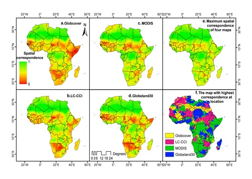
2.1. Global Land Cover Maps

The GLC maps included in this study are: Globcover, LC-CCI, MODIS and Globeland30 maps for the year 2010 (2009 for Globcover). The Globcover project of the European Space Agency (ESA) provided a GLC map for 2009 based on 300 m resolution MERIS satellite data [25]. This map has an LCCS (United Nations Land Cover Classification System) based legend with 22 classes and the thematic overall accuracy of the Globcover-2009 was reported as 70.7% based on 1484 homogenous sample sites [26].

Recently, ESA’s Land Cover-CCI (LC-CCI) project delivered three consecutive GLC maps for the epochs of 2000, 2005 and 2010 at 300 m resolution using the MERIS data archive [27]. These maps were specifically targeted to meet the requirements of climate modelers. The maps also have an LCCS based legend with 22 classes. The overall thematic accuracy of the LC-CCI 2010 map was 74.4% based on the same reference sample as the Globcover-2009 validation.

Using data from the Moderate Resolution Imaging Spectroradiometer (MODIS), Boston University provided annual MODIS Collection-5 GLC maps at 500 m resolution [28]. The MODIS GLC maps have five legends including a legend based on the International Geosphere-Biosphere Programme (IGBP) classification scheme with 17 classes. The accuracy of the MODIS GLC map of 2010 has not yet been assessed. However, based on cross-validation using the training dataset, Friedl et al. [28] reported an overall accuracy of 74.8% for the 2005 map.

The GlobeLand30 project of the Ministry of Science and Technology of China generated a GLC map for the year 2010. The GlobeLand30 map was derived from 30 m resolution multispectral images of Landsat TM and ETM+ as well as the Chinese Environmental Disaster Alleviation Satellite (HJ-1). We used the 250 m resolution version of Globeland30, which contains LC class fraction information. This map has 10 LC classes. The overall accuracy of the map has been reported to be 83.5% [3]. All above-mentioned map accuracies concern the global extent, and for specific regions such as Africa different accuracies are expected. Table 1 [3,26,27,28] provides a summary of the used GLC maps.

Table 1. A summary of GLC maps used for comparison.

GLC Map	Globcover	LC-CCI	MODIS	Globeland30
Spatial resolution at the Equator	300 m	300 m	500 m	250 m
Input data	MERIS: Bi-monthly from 10-day composites	MERIS global SR composite, SPOT-VGT time series (for updating)	MODIS: Monthly EVI, LST and 7 bands from 8-day composites	Landsat TM, ETM+ and HJ-1 multispectral images
Time of data collection	2009	2008–2012	2010	2010 ± 1 year
Classification method	(Un)supervised spatio-temporal clustering; expert-based labeling	Unsupervised spatio-temporal clustering; machine learning classification	Supervised decision tree boosting	Integration of pixel and object based classification and Knowledge based interactive verification
Classification scheme	LCCS based:22 classes	LCCS based: 22 classes	5 different legends including the IGBP (17 classes)	10 classes
Reference	[26]	[27]	[28]	[3]

Table 1. A summary of GLC maps used for comparison.

GLC Map	Globcover	LC-CCI	MODIS	Globeland30
Spatial resolution at the Equator	300 m	300 m	500 m	250 m
Input data	MERIS: Bi-monthly from 10-day composites	MERIS global SR composite, SPOT-VGT time series (for updating)	MODIS: Monthly EVI, LST and 7 bands from 8-day composites	Landsat TM, ETM+ and HJ-1 multispectral images
Time of data collection	2009	2008–2012	2010	2010 ± 1 year
Classification method	(Un)supervised spatio-temporal clustering; expert-based labeling	Unsupervised spatio-temporal clustering; machine learning classification	Supervised decision tree boosting	Integration of pixel and object based classification and Knowledge based interactive verification
Classification scheme	LCCS based:22 classes	LCCS based: 22 classes	5 different legends including the IGBP (17 classes)	10 classes
Reference	[26]	[27]	[28]	[3]

All the GLC maps were cropped to the extent of Africa. The MODIS and Globeland30 maps were resampled to 0.00278 degrees resolution using nearest neighbor assignment to match the resolution of the Globcover and LC-CCI maps. The legends of the GLC maps were harmonized into eight general LC classes following the approach of Herold et al. [4], which provides a table for harmonizing input classes into 13 general LC classes using LCCS-based legend translation protocols. Since the Globeland30 map does not have detailed forest classes, we used a single general forest class only (Table 2). Figure 1 presents the four GLC maps with the harmonized legend.

Table 2. General land cover classes and corresponding classes of the GLC datasets.

Code	Land Cover Class	Globcover	LC-CCI	IGBP (MODIS, STEP and VIIRS)	GLC2000	Geo-Wiki	GLCNMO
1	Forest	40–110, 160, 170	50–100, 160, 170	1–5, 8, 9	1–10	1	1–5
2	Shrubland	130	120	6, 7	11, 12	2	7
3	Grassland	120, 140	110, 130, 140	10	13	3	8, 9
4	Cropland (incl. mixtures)	11–30	10–40	12, 14	16–18	4	11, 12, 13
5	Wetland vegetation	180	180	11	15	6	15
6	Urban/built up	190	190	13	22	7	-
7	Bare/sparse vegetation	150, 200	150, 200	16	14, 19	9	10, 16, 17
8	Water and Snow/Ice	210, 220	210, 220	15, 17	20, 21	8, 10	-

Table 2. General land cover classes and corresponding classes of the GLC datasets.

Code	Land Cover Class	Globcover	LC-CCI	IGBP (MODIS, STEP and VIIRS)	GLC2000	Geo-Wiki	GLCNMO
1	Forest	40–110, 160, 170	50–100, 160, 170	1–5, 8, 9	1–10	1	1–5
2	Shrubland	130	120	6, 7	11, 12	2	7
3	Grassland	120, 140	110, 130, 140	10	13	3	8, 9
4	Cropland (incl. mixtures)	11–30	10–40	12, 14	16–18	4	11, 12, 13
5	Wetland vegetation	180	180	11	15	6	15
6	Urban/built up	190	190	13	22	7	-
7	Bare/sparse vegetation	150, 200	150, 200	16	14, 19	9	10, 16, 17
8	Water and Snow/Ice	210, 220	210, 220	15, 17	20, 21	8, 10	-

Figure 1. Global land cover maps used in the analyses.

Figure 1. Global land cover maps used in the analyses.

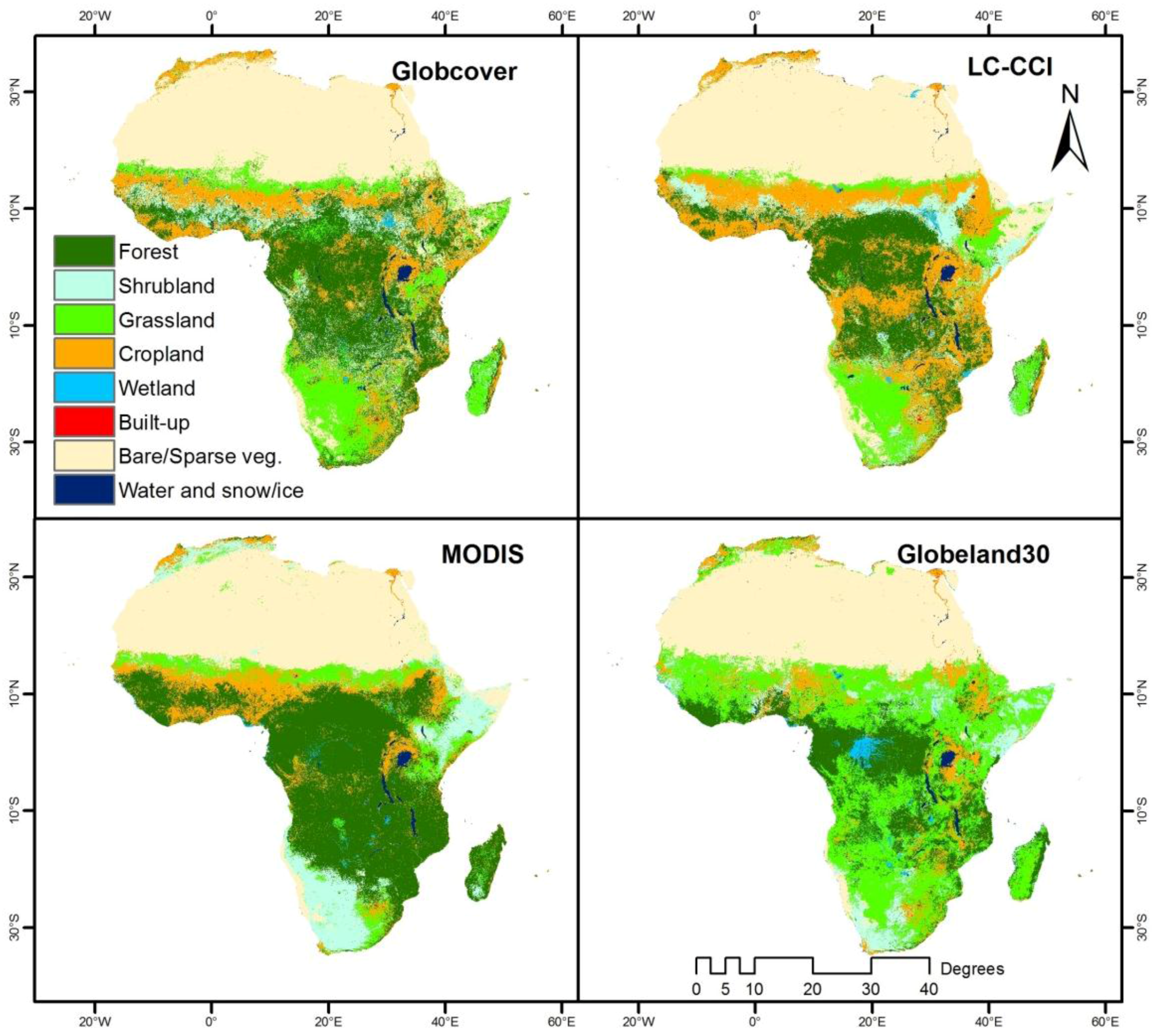
2.2. Reference Datasets

The reference datasets used in this work are denoted as: GLC2000rd, GLCNMOrd, Geo-Wikird, MODIS/STEPrd, VIIRSrd and the Globcover-2005rd. The subscript “rd” is added here to avoid potential confusion between LC maps and reference datasets. GLC2000rd concerns the consolidated version (11 LC classes) of the reference dataset generated for validating the Global Land Cover 2000 map [29,30]. GLCNMOrd refers to the calibration dataset of Global Land Cover by National Mapping Organizations, which was used to generate a GLC map for 2003 [31]. This dataset employs 14 LC classes, which were assigned to sample sites by international experts. MODIS/STEPrd has been used to calibrate the MODIS collection 4 and 5 GLC maps [28]. This dataset was developed and updated by Boston University and it has 17 LC classes according to the IGBP legend. Boston university also created VIIRSrd (Visible Infrared Imaging Radiometer Suite), which was used to validate the VIIRS surface type products [18,32]. The reference LC of this dataset was assigned by visual interpretation of very high-resolution images using the same classes as MODIS/STEPrd. Geo-Wikird was developed through a volunteer based online platform and volunteers’ interpretation of the reference LC was validated by a group of experts [33]. Globcover 2005rd is a re-interpreted version of the reference dataset that was built for validating the Globcover 2005 GLC map [6,34]. Detailed information on the characteristics of the available reference datasets are provided in [35]. Although there are temporal differences between the used datasets, we deemed these to be of minor importance, since errors owing to LC changes over the time frame are negligible compared to misclassification errors of the GLC maps.

These reference datasets are publicly accessible through the GOFC-GOLD Reference data portal, Geo-Wiki portal and International Steering Committee for Global Mapping [18,31,33].

To cope with differences in sample site areas across the reference datasets, we assumed that the LC of the sample site corresponds to the LC of the centroid of that sample sites. Reference data were then compared to the LC classes of the GLC maps at the centroids of the reference sites. For the combined reference dataset, the legends of all reference datasets were harmonized into the eight general classes listed in Table 2 to correspond with GLC map harmonization as given in Section 2.1.

In total, 3887 sample sites within Africa were used in this study. Based on this reference dataset, model-based geostatistical analysis was used since in contrast to design-based inference it does not require a probability sampling design. Figure 2 shows the sample distribution of each reference dataset (left) and the reference LC classes (right).

Figure 2. Spatial distribution of the reference datasets (left) and reference LC classes (right).

Figure 2. Spatial distribution of the reference datasets (left) and reference LC classes (right).

3. Method

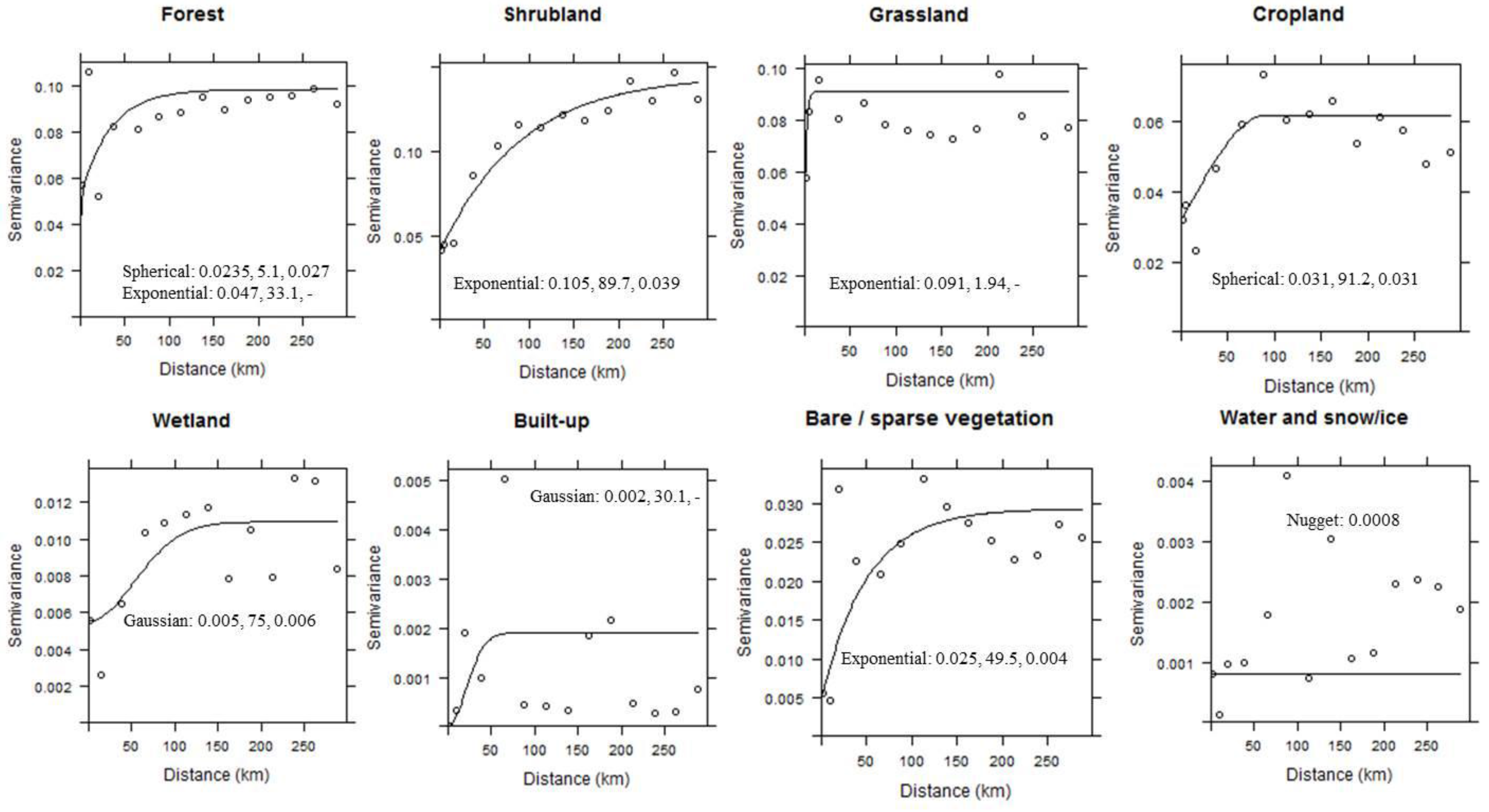
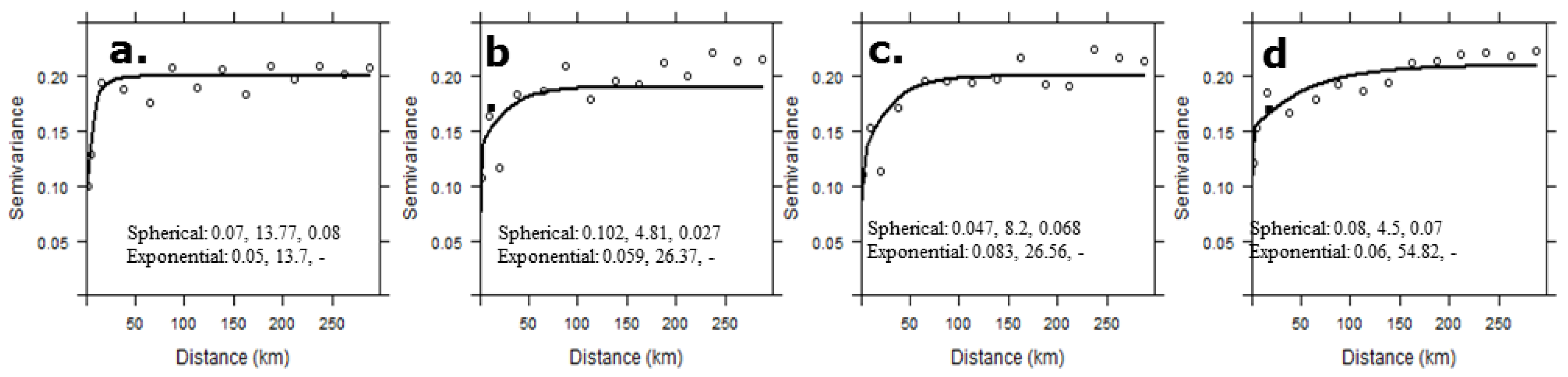
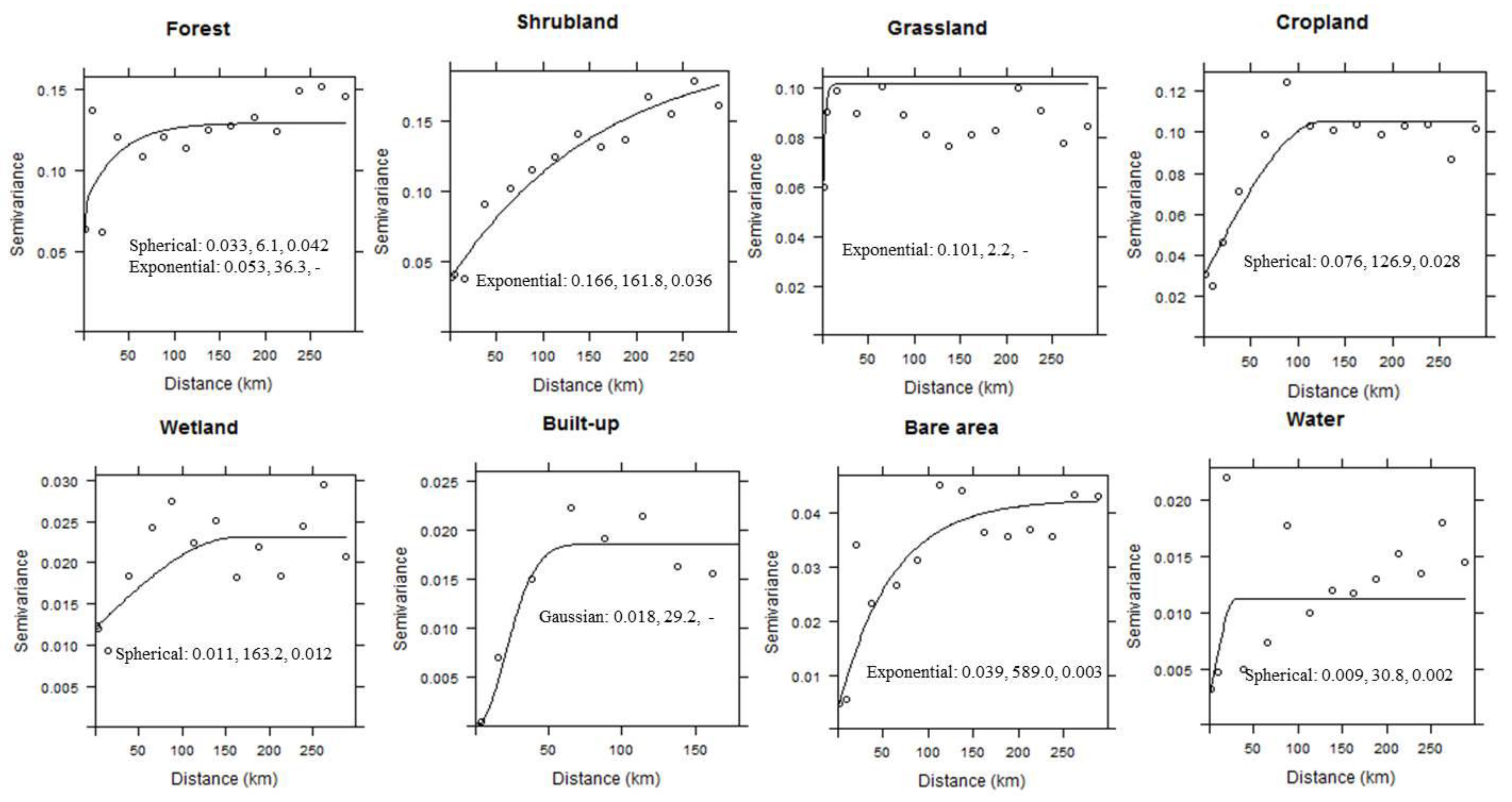
3.1. Spatial Correspondence Assessment

To assess spatial accuracy (spatial variation in map accuracy) we analyzed the spatial correspondence of the GLC map with the reference dataset. Correspondences between GLC maps and reference data were indicator coded. If the LC class of the reference sample site matched with that of a map, an indicator code 1 was assigned to that sample site. Conversely, an indicator code 0 was given to sites where the mapped LC differed from the reference class. Next, we analyzed spatial autocorrelation of the indicator-coded data (correspondence with reference LC) using indicator semivariograms. Nested variogram models were fitted to experimental semivariogram data obtained by the method of moment approach with binning of 3–5, 10–15 and intervals of 25 km [36]. Variograms were fitted by weighted least squares using N_j/h²_j as weights, where N_j denotes the number of point pairs in the j-th lag and h_j is the corresponding lag distance.

Spatial correspondence maps were created for each GLC map for Africa at 0.00278 degrees resolution (300 m at the Equator) by indicator kriging [37] using the gstat package in R [38]. The spatial correspondence maps depict the local correspondence values ranging between 0 and 1, which denotes the local probability that a particular map is correct. Figure 3 demonstrates the semivariograms of spatial correspondence for the GLC maps and used fitted models for the indicator kriging. To restrict the size of the kriging system, kriging was done with the nearest 50 observations.

Figure 3. Semivariograms and fitted models for spatial correspondence of the Globcover (a); LC-CCI (b); MODIS (c); and Globeland30 (d) maps (model parameters: partial sills, range and nugget).

Figure 3. Semivariograms and fitted models for spatial correspondence of the Globcover (a); LC-CCI (b); MODIS (c); and Globeland30 (d) maps (model parameters: partial sills, range and nugget).

3.2. GLC Dataset Integration

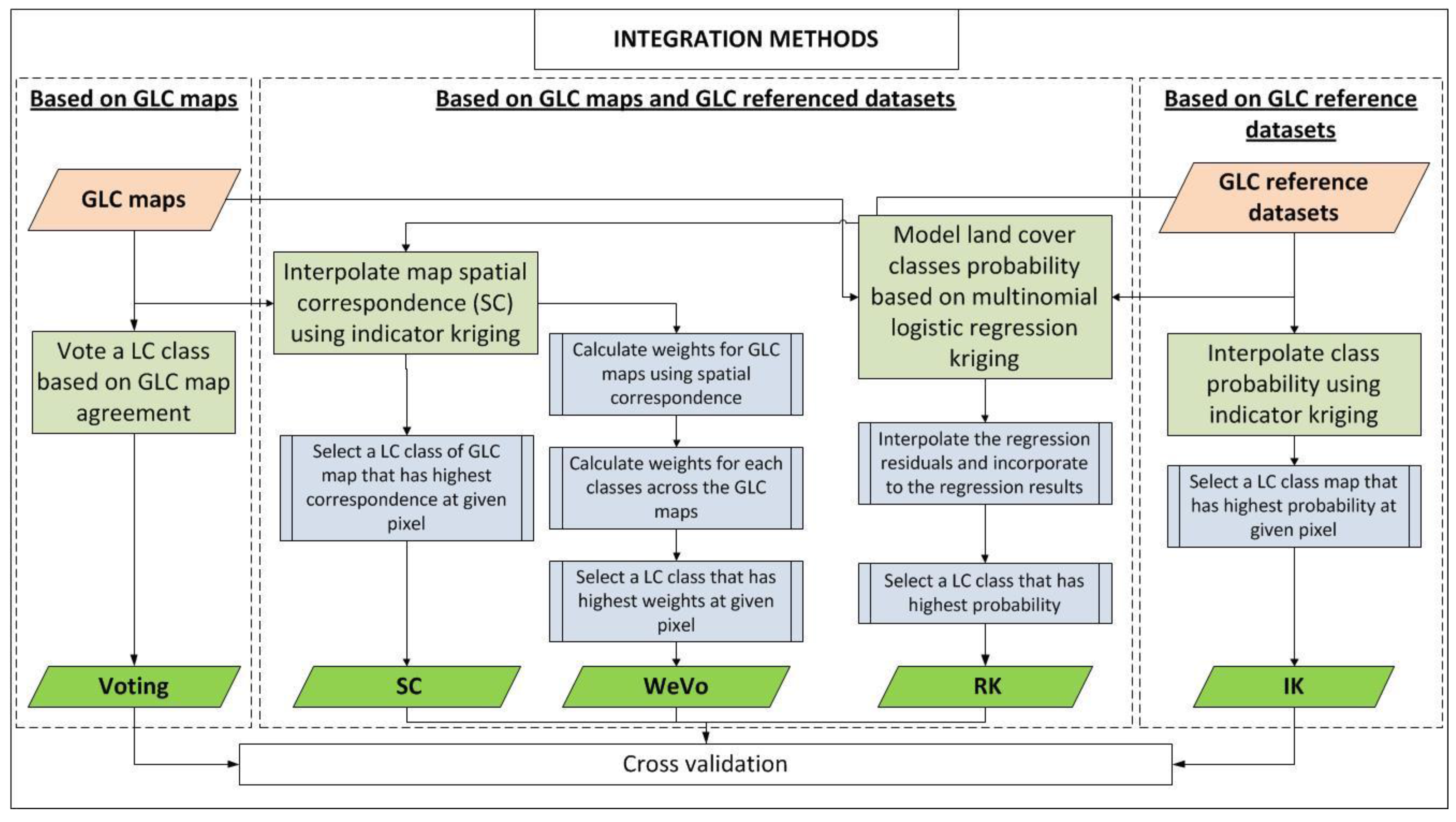
Analyzing the local variation in map accuracy is useful for obtaining information on where a map is accurate and where not, and this information can be valuable in creating an improved GLC map. Previous integration efforts of GLC maps did not focus on the local variation in map accuracy except the work of See et al. [9], who analyzed GLC maps with highest correspondence at a coarser grids of 0.25 degrees using geographically weighted kernel approach. However, the resulting integrated maps have artifacts in the pattern of LC classes that are caused by the coarse grid kernels [9].

Our study extends the principle of considering local variation of map accuracies and LC class probabilities for creating an improved LC map. We used a geostatistical approach to assess and model the spatial dependence of map accuracy and class probabilities. We compared different integration methods, as depicted in Figure 4, which represent a variety of choices concerning the use of input datasets. These include methods based on spatial correspondence of the GLC maps, agreement amongst input maps and the LC class presence probabilities, i.e., using both the GLC maps and the reference datasets. In addition, methods based on a conventional voting approach [10], i.e., without using reference data, and a geostatistical method that relies only on the reference data, i.e., without using the GLC maps, were also compared. We first applied all methods to the sample locations. After selecting the integration method with highest correspondence by cross-validation (see Section 3.2.6), the latter was applied to the full extent of Africa.

Figure 4. Conceptual diagram of different integration methods.

Figure 4. Conceptual diagram of different integration methods.

The following subsections describe the integration methods used in this study.

3.2.1. Voting

This integration method only uses the GLC maps as input. At each pixel location, the LC class corresponding to the majority of the mapped LC classes of the four input maps was assigned. In case of a tie, the LC class of a map that has the highest overall reported accuracy was assigned. Since there is no information on the accuracy of these maps in Africa, the reported global confusion matrices of the maps (see Table 1 for reference) were converted into confusion matrices for the eight generalized classes and the corresponding overall accuracy was calculated. The global accuracies at generalized class level were computed as 66%, 75.3%, 85.4% and 83.5% for the Globcover, LC-CCI, MODIS and Globeland30, respectively. Accordingly, the MODIS LC class was assigned in case of ties.

3.2.2. Spatial Correspondence (SC)

This method (SC) uses both the GLC maps and reference datasets as inputs. Based on the spatial correspondence map for each GLC map resulting from the method described in Section 3.1, we selected the LC class of the map that has the highest spatial correspondence value at a pixel location.

3.2.3. Weighted Voting (WeVo)

Weighted voting (WeVo) also uses both the GLC maps and the reference datasets. We created normalized weight maps using the spatial correspondence maps of the GLC maps. Let sc_i(x) denote the spatial correspondence of the i-th GLC map (i = 1, …, 4) at location x. W_i(x), the weight assigned to map i at location x, is then:

$$W_i\left(x\right)=\frac{s{c}_i\left(x\right)}{{\sum }_{i=1}^{4}s{c}_i\left(x\right)}$$

(1)

LC classes were dummy coded into multiple 1 or 0 indicators, where 1 indicates that a LC class k (k = 1, …, 8) is present and 0 means k is absent. Using these indicator values, we assigned the weights to the classes mapped on each of the GLC maps. For each LC class k, a total weight of the LC class at x location was created by summing the class weights of the four GLC maps (Equations (2) and (3)).

$$w_{i,k}\left(x\right)=W_i\left(x\right)\ast k_i\left(x\right)$$

(2)

$$W_k\left(x\right)={\displaystyle \sum _{i=1}^4}{w}_{i,k}\left(x\right)$$

(3)

where k is the LC class, W_k(x) is the total weight of the LC class at location x, and W_i,k(x) is class weight of the GLC map. A LC class with highest total weight at a location (Wk(x)) was then selected for this method.

3.2.4. Regression Kriging (RK)

Regression kriging (RK) similarly uses both the GLC maps and the reference datasets. The general trend of probabilities of presence of LC classes were predicted using a multinomial logistic (MNL) regression model. These were locally adjusted by interpolating indicator residuals by simple kriging (Equation (4)).

$$p_k\left(x\right)={\pi }_k\left(x\right)+{\epsilon }_k\left(x\right)$$

(4)

where p_k(x) denotes the presence probability of a LC class at location x, π_k(x) is a predicted probability trend of an LC class that was obtained by MNL regression [39] and ε_k(x) is the indicator residuals for that class. The latter was obtained by simple kriging. MNL regression also uses indicator values of the LC classes. There is an indicator variable for all but one class [39]. The MNL regression estimated a separate binary logistic regression model for each of these indicator variables. For each indicator variable (k = 2, …, 8), the log odds function for predicted probability is:

$${\mathsf{\eta }}_k\left(x\right)=\text{log}\left(\frac{{\pi }_k\left(x\right)}{1-{\pi }_k\left(x\right)}\right)={\beta }_{0k}+{\beta }_{1k}{h}_1\left(x\right)+{\beta }_{2k}{h}_2\left(x\right)+\dots +{\beta }_{jk}{h}_j\left(x\right)$$

(5)

where h_j (with j = 1, …,4) are the explanatory variables (LC class of the four GLC maps at sample locations), β_1k … β_jk are the regression coefficients and β_0k is the intercept. To ensure that all probabilities are in the interval [0,1] and that the probabilities sum to 1, Equations (6) and (7) were used [39].

$${\pi }_k\left(x\right)=\frac{\text{exp}\left({\mathsf{\eta }}_k\left(x\right)\right)}{{\sum }_{k=2}^8\text{exp}\left({\mathsf{\eta }}_k\left(x\right)\right)}$$

(6)

$${\pi }_1\left(x\right)=1/{\displaystyle \sum _{k=2}^8}\text{exp}\left({\mathsf{\eta }}_k\left(x\right)\right)$$

(7)

where exp(η_k(x)) denotes the odds of class k at location x. This was implemented using the nnet package in R [40].

Next, regression residuals at sample locations were calculated and simple kriging was used to interpolate the regression residuals (ε_k(x)) at un-sampled locations for all classes except water. For the water class, no spatial correlation was observed on the regression residuals based on the experimental semivariogram. Semivariograms were fitted using the same method as described in Section 3.1. Figure 5 demonstrates the semivariograms of regression residual for the LC classes and fitted variogram models used for kriging.

Figure 5. Semivariograms and fitted models for residual kriging.

Figure 5. Semivariograms and fitted models for residual kriging.

After adjusting the predicted probabilities with residual kriging, any probability outside the interval [0, 1] was set to the closest bound, zero or one. Subsequently, the estimates pk(x) k = 1, …, K were normalized by their sum to meet the condition ${\sum }_{k=1}^K{p}_k\left(x\right)=1$ [22]. A pixel was assigned to the LC class having the highest probability.

3.2.5. Indicator Kriging (IK)

For comparison, the last integration method was based on indicator kriging that uses only the reference datasets. Based on these indicator variables for LC classes, the presence probability of LC classes was modeled at the test locations of the cross validation (see next section).

Figure 6 shows the semivariograms and the fitted models used for modeling LC classes presence probability based on indicator kriging (Section 3.1). A LC class with highest modeled probability was selected for this method.

Figure 6. The semivariograms and fitted models used for Indicator Kriging.

Figure 6. The semivariograms and fitted models used for Indicator Kriging.

3.2.6. Cross-Validation

The performance of these methods was analyzed using 10 fold cross-validation. The reference sample sites were partitioned into 10 random subsamples. Nine subsamples (3498 ± 1 sample sites) were used to train the integration methods and one subsample (389 ± 1 sample sites) was used to validate the method performance by assessing the overall correspondence between the reference LC and LC from method outputs. This step was repeated 10 times so that each subsample was used for method training as well as validation and each sample site was used for validation exactly once. The median percentage of integrated LC classes locally corresponding with reference subsamples was then calculated. Note that these values should not be confused with the overall accuracy of LC maps since they are based on cross-validation using a heterogeneous sample rather than comparison against an independent reference dataset obtained by probability sampling. Based on the cross-validation results, the integration method having the highest correspondence with the reference LC was selected for creating an improved LC map.

4. Results and Discussions

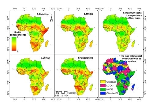
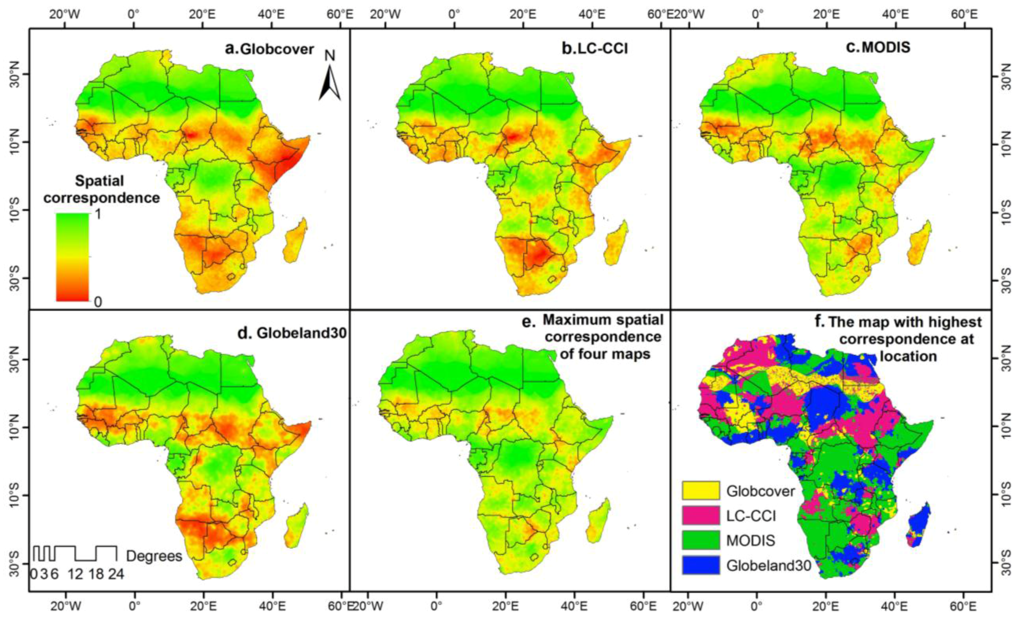
4.1. Spatial Correspondence of GLC Maps in Africa

The spatial correspondences of the GLC maps based on indicator kriging are provided in Figure 7. In terms of the spatial correspondence with reference LC, all four maps show similar trends. The Sahara desert and tropical rainforest regions were mapped with high correspondence, whereas the Sahel, and dry and moist savannah regions were generally mapped with low correspondence. In the latter regions, some differences in terms of spatial correspondence of the maps could be observed. For instance, the LC-CCI showed higher spatial correspondence related to cropland areas in Morocco and northern Algeria, Ethiopia, Eritrea, Sudan, Zambia, Zimbabwe and Angola. In other regions, the LC-CCI map tends to over-represent the cropland class. The MODIS map had higher correspondence in Somalia, Kenya, Mozambique, Namibia, Botswana and western part of South Africa as it has more shrubland areas. The Globeland30 map had higher correspondence in the tropical forest regions of western Africa, Chad, Uganda, Tanzania, Madagascar, and eastern part of South Africa related to grassland areas. A general tendency of over-representing the grassland class was also observed for the Gloebeland30 in other regions. These differences are also highlighted in Figure 7f, which illustrates the maps with highest correspondence at a given location. The strengths of the GLC maps over one another in different regions show the potential of creating an improved GLC map by integrating them.

Figure 7. Spatial correspondence of the GLC maps (a–d), maximum correspondence (e) and the map with highest correspondence (f).

Figure 7. Spatial correspondence of the GLC maps (a–d), maximum correspondence (e) and the map with highest correspondence (f).

Figure 7e shows the maximum spatial correspondence of the four maps and this demonstrates that the Sahel and dry savannah regions of Africa were mapped with the lowest spatial correspondence in all four maps. This could be due to the presence of multiple LC classes (i.e., heterogeneous landscapes) in transition zones of major ecosystem, which are difficult to classify correctly, owing to spectral and thematic similarity. GLC maps often do not agree in these regions [4,24]. These regions should be the main focus of map improvement efforts including the development of new GLC maps.

Information on the spatial variation in map correspondence is useful in uncertainty assessments of applications that use GLC maps and in map improvement efforts. It also provides confidence in using the GLC maps for regions with high map spatial correspondence and limited regional data availability.

In terms of correspondence with reference LC classes aggregated over the entire African continent, MODIS had highest correspondence (63%) followed by Globeland30 (57.2%), LC-CCI (55.5%) and finally Globcover (50.8%).

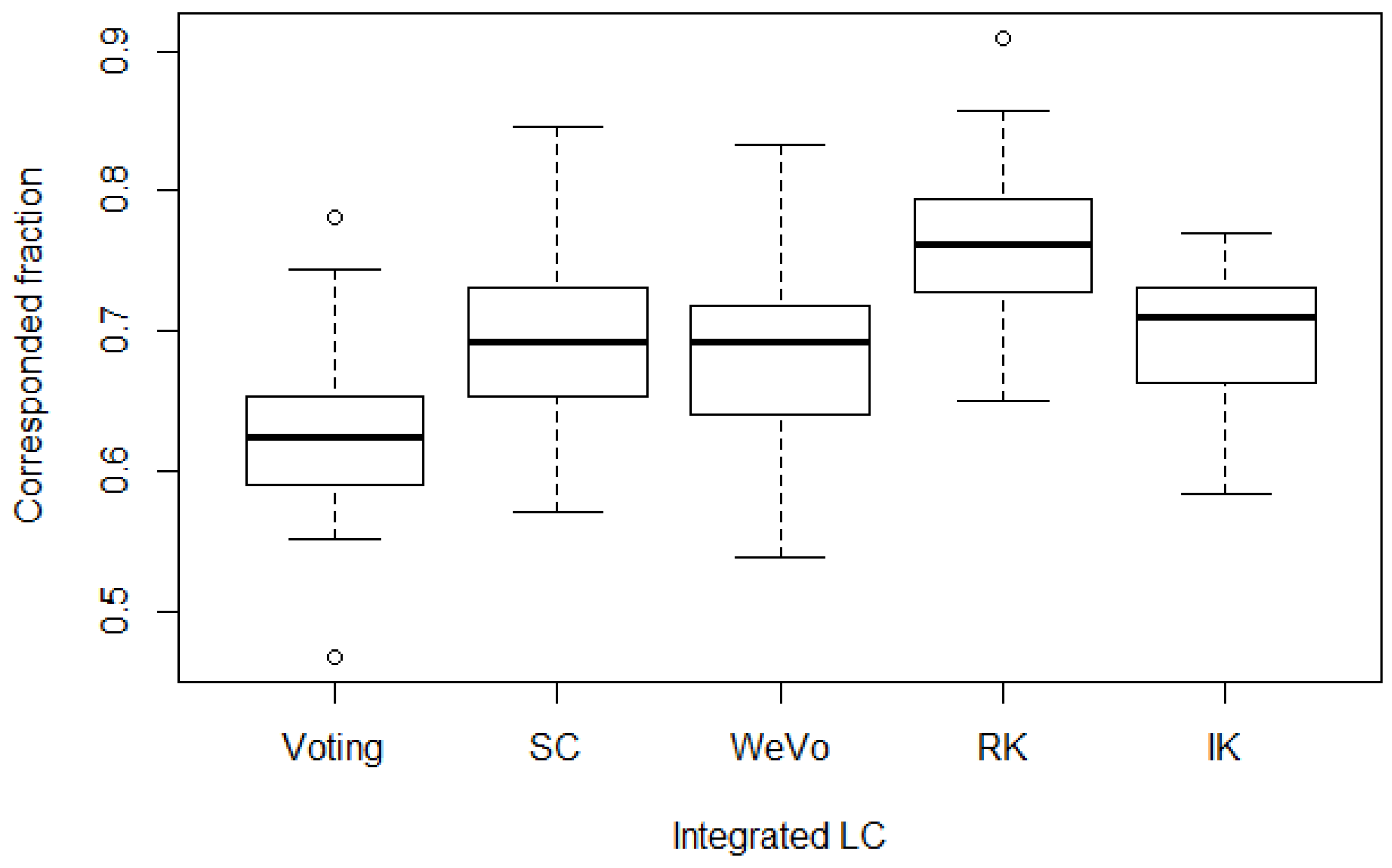
4.2. GLC Dataset Integration Methods

The result of the 10 fold cross-validation assessing the performances of the integration methods for an improved GLC map is presented in Figure 8. The medians of correspondence of integrated LC with reference data varied from 62.3%–76% across different integration methods (Figure 8). The integration method based on only the GLC maps (Voting) resulted in the lowest correspondence of 62.3%, which is less than the 63% of the MODIS map. A possible explanation is that the voting rule will assign a pixel to a wrong class if the majority of input maps agrees to that class.

Figure 8. Correspondence of integrated LC with reference sample LC (10-fold cross validation).

Figure 8. Correspondence of integrated LC with reference sample LC (10-fold cross validation).

The integration methods based on both the GLC maps and reference datasets resulted in 67.5%–76% correspondence with the reference LC, which is at least 4.5%–13% higher than the correspondence of the input maps. The RK method produced the highest correspondence (76%) compared with the other integration methods. The RK method ensures to reduce the classification errors as much as possible by exploiting the “best” of the available data i.e., modeling global trends of the LC class probabilities using the GLC maps as explanatory variables and calculating the local deviations from the global trends near reference points using spatial correlation of the residuals between trends and reference data [41]. The smaller sill values of the fitted models for residual kriging compared to that of the indicator kriging (Figure 5 and Figure 6) are indicative of the contribution of MNL regression in explaining the LC class probabilities [41]. This also justifies the use of residual kriging to model the remaining unexplained spatial variation of LC class probabilities.

Figure 8 shows that all methods using reference data produced higher correspondence than the Voting method. This could have been expected, since more data are being used. However, even IK that uses only reference data produced better correspondence than Voting. This underlines the importance of reference data in map improvement efforts. The spread in the cross-validation results obtained by IK is expected, since cross-validation repeatedly removes difference subsets of the reference data while IK is based on the reference data only. The intermediate positions of SC and WeVo can be explained by the fact that they employ map spatial correspondence and agreements amongst input maps, rather than class specific probabilities as considered in the RK method. Using different methods, See et al. [9] also observed limitations in using map spatial correspondence and agreement amongst map for integration. Our results demonstrate the advantage of using both the GLC maps and the reference data for integration where data abound while relying on the GLC maps only in places where the reference data is sparse.

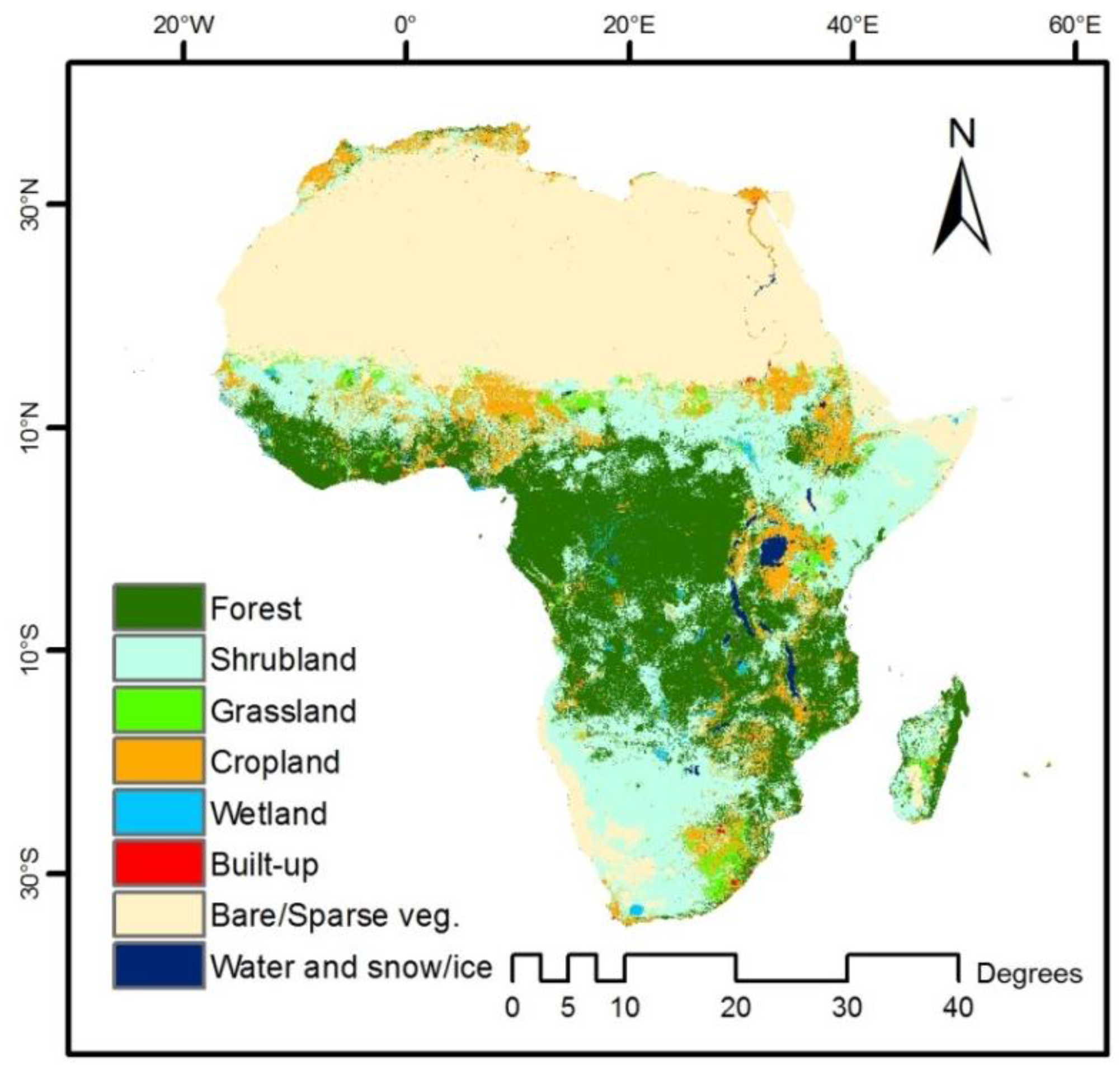
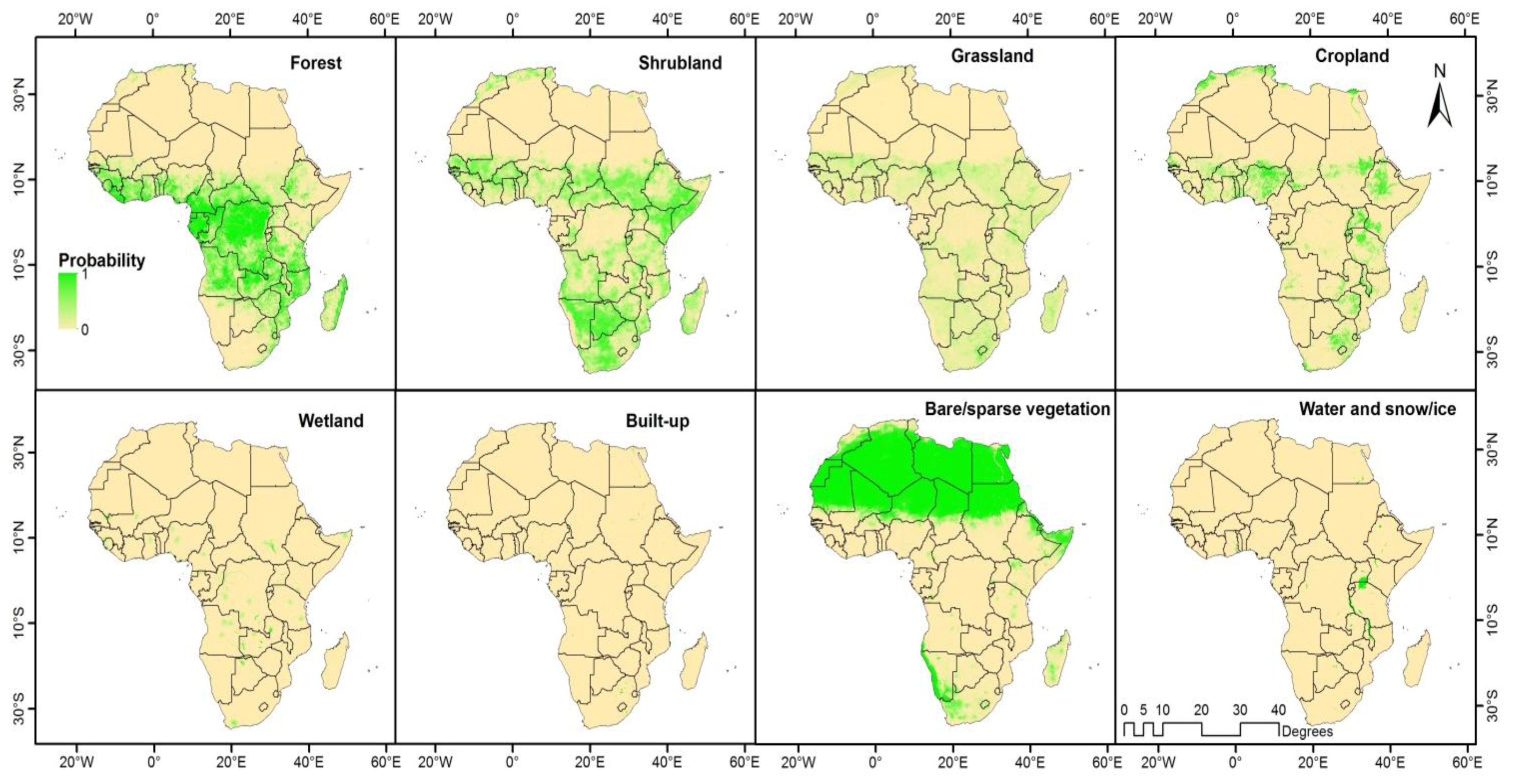
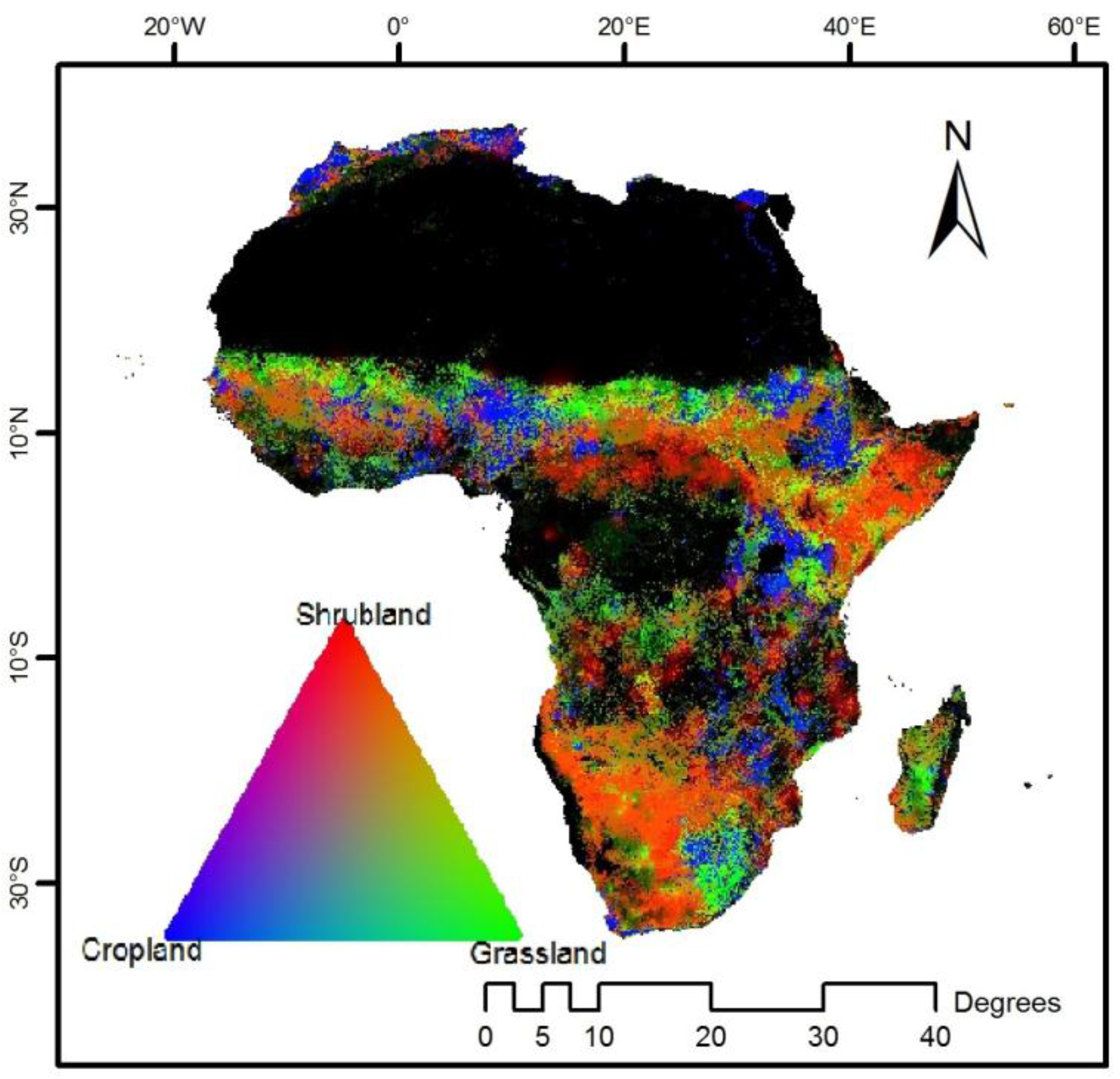
4.3. Integrated LC and LC Probability Maps of Africa

Since the RK integration method had the highest correspondence with reference LC (see Section 4.2), we used this method to create an integrated LC map of Africa using the input GLC maps and reference datasets (Figure 9). The integrated map had similar pattern to the input maps in terms of forest and bare/sparse vegetation classes. The main difference between the integrated map and the input maps is the fact that more area of shrubland and relatively less area of cropland and grassland are present. On the other hand, the general patterns of the LC classes were similar to those of the reference data (Figure 2 right).

Figure 9. Integrated LC map based on RK method.

Figure 9. Integrated LC map based on RK method.

Table 3 compares class-specific correspondences of RK integration and the input maps with the reference dataset. All LC class correspondences were derived by cross-validation (see Section 4.2). The RK method improved class correspondences for LC classes excluding forest, cropland, grassland and built-up. The forest, grassland and cropland classes were over-represented in the MODIS, Globeland30 and LC-CCI maps, respectively.

Table 3. Class-specific correspondences of RK integration and the input GLC maps with reference data.

	Globcover	LC-CCI	MODIS	Globeland30	RK
Forest	71.1	67.3	90.2	63.7	84.9
Shrubland	11.9	21.3	26.9	17.3	70.8
Grassland	18.4	18.9	27.1	70.4	41.1
Cropland	57.7	79.2	66.7	76.0	75.0
Wetland	25.0	31.5	59.8	52.2	67.0
Built-up	74.5	91.5	78.7	91.5	89.4
Bare/sparse vegetation	76.0	78.5	75.0	72.0	87.6
Water and snow/ice	80.0	80.0	70.0	78.0	86.7
Total	50.7	55.4	62.8	57.1	76.3

Table 3. Class-specific correspondences of RK integration and the input GLC maps with reference data.

	Globcover	LC-CCI	MODIS	Globeland30	RK
Forest	71.1	67.3	90.2	63.7	84.9
Shrubland	11.9	21.3	26.9	17.3	70.8
Grassland	18.4	18.9	27.1	70.4	41.1
Cropland	57.7	79.2	66.7	76.0	75.0
Wetland	25.0	31.5	59.8	52.2	67.0
Built-up	74.5	91.5	78.7	91.5	89.4
Bare/sparse vegetation	76.0	78.5	75.0	72.0	87.6
Water and snow/ice	80.0	80.0	70.0	78.0	86.7
Total	50.7	55.4	62.8	57.1	76.3

Probability maps for each LC class produced by means of RK are shown in Figure 10. While distinct high probability areas of forest, bare/sparse vegetation and water and snow/ice classes can be observed in Figure 10, the Sahel and savannah areas are represented by multiple classes such as shrubland, grassland and cropland, which had similar probabilities.

Figure 10. Probability maps of LC classes.

Figure 10. Probability maps of LC classes.

As the LC classes of the integrated map were selected based on the maximum presence probability, shrubland class superseded the grassland class by having a higher probability value in these regions and therefore more area of shrubland is observed in Figure 9. This can be observed in Figure 11, which shows the combination of class probabilities of shrubland (red), grassland (green) and cropland (blue). Substantial areas in orange color highlight the combination of shrubland and grassland as probable classes with the presence probability of shrubland is higher than that of grassland (Figure 11). In contrast, the extent of areas with only shrubland as probable class (red) is considerably less. The combination of grassland and cropland as probable classes is shown in cyan color that can mostly be observed in the northern part of Sahel and eastern part of South Africa. Figure 11 illustrates the complexity of landscape with multiple probable class in the Sahel and savannah areas. For studies regarding these areas, consulting with the presence probability maps of the LC classes are recommended.

Figure 11. RGB image of class probabilities of shrubland, grassland and cropland. Dark shades represent areas where none of these three classes has a presence probability.

Figure 11. RGB image of class probabilities of shrubland, grassland and cropland. Dark shades represent areas where none of these three classes has a presence probability.

The presence probability maps of the LC classes are helpful in understanding the uncertainties in class assignment in the integrated maps as well as the complexity of heterogeneous landscapes.

4.4. On the Use of Available Reference Datasets for Integration

This study made use of GLC reference datasets that were developed from different initiatives. The combined reference dataset has rather dense spatial distribution over a large portion of the African continent, which is beneficial for geostatistical interpolation. In the Sahara desert, sample density was lower. Nevertheless, correspondence with the reference LC was high in this region (Figure 7) as bare areas are usually mapped with high accuracy [4]. One should be cautious when integrating different reference datasets as they may have discrepancies in their legends, sampling design and response design (i.e., sample site area) [35]. To reduce the legend discrepancies of the reference datasets, we harmonized their legends into a common system with 8 general classes. However, there may be some inconsistencies in the reference datasets due to the discrepancies in the definition of LC classes.

Another issue is that reference datasets use different spatial supports. Our approach of using the centroids of reference sites provided a practical solution. However, differences in spatial support among reference data sets (and maps) are often a source of uncertainty about the true land cover. Block kriging and area-to-point [42,43] have been proposed for dealing with different spatial supports. Note that area-to-point kriging requires semivariograms at the fine spatial resolution, which may be difficult to acquire. Last, but not least, the integration approach of the reference datasets demonstrated in this study can be used for other studies that use geostatistical approaches. Since some reference datasets are not based on probability sampling, design-based statistical inference cannot be used. Moreover, design-based statistical inference using multiple reference datasets with different statistical sampling designs requires known inclusion probabilities [44].

5. Conclusions

This study utilized the available GLC reference datasets from the GOFC-GOLD, Geo-Wiki and the International Steering Community for Global Mapping. These datasets were originated from various institutions and the diversity of the reference datasets characters (e.g., legend and sample site area) makes them challenging to be integrated and reused for other studies. Our study provides an example of dealing with such diversities by harmonizing the thematic and spatial support differences of the reference datasets and using them for model-based geostatistical estimations. Further initiatives on generating better and more consolidated GLC maps can be useful to reduce discrepancies and uncertainty caused by legend harmonization. The advantages of including different reference datasets for integration were demonstrated in this study. Such information is useful as more reference datasets are becoming available to the public thanks to GLC mapping and validation communities [18,19].

Our study analyzed and compared the spatial variation in thematic correspondence of GLC maps, namely the Globcover 2009, LC-CCI 2010, MODIS 2010 and Globeland30, with the reference datasets. Based on the spatial autocorrelation structure of map correspondence, we modeled the spatial correspondence of the GLC maps as a measure of spatial accuracy. The comparison of the spatial correspondence maps demonstrated generally uncertain areas in LC mapping in Africa that need attention for improvement efforts while the preferences for GLC maps varied spatially. This finding demonstrates a motivation of integrating GLC maps based on their spatial variation in map correspondence in order to create an improved GLC map.

Aiming to create an improved LC map, we tested five different methods which are based on multiple GLC maps and reference datasets. The integration methods that employed both the GLC maps and the reference datasets resulted in 4.5%–13% higher correspondence with the reference LC classes than that of the input GLC maps. These methods exceeded the other two methods by making best use of the available data by calibrating the GLC maps with the help of reference datasets and relying on the GLC maps in places where the reference dataset is sparse. This result illustrates the benefit of using existing reference datasets and geostatistical approaches for map integration. In contrast, integration based on the agreement amongst the input maps without questioning their spatial correspondence did not result in improved correspondence with reference LC. Nevertheless such approaches are commonly adopted for map integration efforts.

The RK method, which ensures to reduce the classification errors as much as possible through MNL regression and kriging of the regression residuals, showed the highest correspondence with reference LC. This method was selected to create an integrated LC map and the LC class probability maps of Africa. Uncertainty in class assignment was higher in heterogeneous areas with mixtures of different LC classes than in homogenous areas. In heterogeneous areas such as the Sahel and dry and moist savannahs, the LC probability maps can be useful. This study was done for the extent of Africa. With increasing computational power and more data coming available, the approach can be extended to global coverage and other datasets can also be included as covariates.

References

1. Verburg, P.H.; Neumann, K.; Nol, L. Challenges in using land use and land cover data for global change studies. Glob. Chang. Biol. 2011, 17, 974–989. [Google Scholar] [CrossRef]
2. Mora, B.; Tsendbazar, N.-E.; Herold, M.; Arino, O. Global land cover mapping: Current status and future trends. In Land Use and Land Cover Mapping in Europe; Springer: Dordrecht, The Netherlands, 2014; pp. 11–30. [Google Scholar]
3. Chen, J.; Chen, J.; Liao, A.; Cao, X.; Chen, L.; Chen, X.; He, C.; Han, G.; Peng, S.; Lu, M. Global land cover mapping at 30 m resolution: A POK-based operational approach. ISPRS J. Photogramm. Remote Sens. 2015, 103, 7–27. [Google Scholar] [CrossRef]
4. Herold, M.; Mayaux, P.; Woodcock, C.E.; Baccini, A.; Schmullius, C. Some challenges in global land cover mapping: An assessment of agreement and accuracy in existing 1 km datasets. Remote Sens. Environ. 2008, 112, 2538–2556. [Google Scholar] [CrossRef]
5. Fritz, S.; See, L.; McCallum, I.; Schill, C.; Obersteiner, M.; van der Velde, M.; Boettcher, H.; Havlík, P.; Achard, F. Highlighting continued uncertainty in global land cover maps for the user community. Environ. Res. Lett. 2011, 6, 044005. [Google Scholar] [CrossRef]
6. Tsendbazar, N.E.; de Bruin, S.; Mora, B.; Schouten, L.; Herold, M. Comparative assessment of thematic accuracy of GLC maps for specific applications using existing reference data. Int. J. Appl. Earth Obs. Geoinf. 2016, 44, 124–135. [Google Scholar] [CrossRef]
7. Kooistra, L.; Groenestijn, A.; Kalogirou, V.; Arino, O.; Herold, M. User requirements from the climate modelling community for next generation global products from land cover cci project. In Proceedings of the ESA-iLEAPS-EGU Joint Conference 2010, Frascati, Italy, 3–5 November 2010.
8. Jung, M.; Henkel, K.; Herold, M.; Churkina, G. Exploiting synergies of global land cover products for carbon cycle modeling. Remote Sens. Environ. 2006, 101, 534–553. [Google Scholar] [CrossRef]
9. See, L.; Schepaschenko, D.; Lesiv, M.; McCallum, I.; Fritz, S.; Comber, A.; Perger, C.; Schill, C.; Zhao, Y.; Maus, V.; et al. Building a hybrid land cover map with crowdsourcing and geographically weighted regression. ISPRS J. Photogramm. Remote Sens. 2015, 103, 48–56. [Google Scholar] [CrossRef] [Green Version]
10. Iwao, K.; Nasahara, K.N.; Kinoshita, T.; Yamagata, Y.; Patton, D.; Tsuchida, S. Creation of new global land cover map with map integration. J. Geogr. Inf. Syst. 2011, 3, 160–165. [Google Scholar] [CrossRef]
11. Tuanmu, M.-N.; Jetz, W. A global 1-km consensus land-cover product for biodiversity and ecosystem modelling. Glob. Ecol. Biogeogr. 2014, 23, 1031–1045. [Google Scholar] [CrossRef]
12. Ge, Y.; Avitabile, V.; Heuvelink, G.B.; Wang, J.; Herold, M. Fusion of pan-tropical biomass maps using weighted averaging and regional calibration data. Int. J. Appl. Earth Obs. Geoinf. 2014, 31, 13–24. [Google Scholar] [CrossRef]
13. Fritz, S.; See, L.; McCallum, I.; You, L.; Bun, A.; Moltchanova, E.; Duerauer, M.; Albrecht, F.; Schill, C.; Perger, C.; et al. Mapping global cropland and field size. Glob. Chang. Biol. 2015, 21, 1980–1992. [Google Scholar] [CrossRef] [PubMed] [Green Version]
14. Avitabile, V.; Herold, M.; Heuvelink, G.; Lewis, S.; Phillips, O.; Asner, G.; Armston, J.; Asthon, P.; Banin, L.; Bayol, N. An integrated pan-tropical biomass map using multiple reference datasets. Glob. Chang. Biol. 2015. [Google Scholar] [CrossRef] [PubMed]
15. Kinoshita, T.; Iwao, K.; Yamagata, Y. Creation of a global land cover and a probability map through a new map integration method. Int. J. Appl. Earth Obs. Geoinf. 2014, 28, 70–77. [Google Scholar] [CrossRef]
16. Comber, A.; See, L.; Fritz, S.; van der Velde, M.; Perger, C.; Foody, G. Using control data to determine the reliability of volunteered geographic information about land cover. Int. J. Appl. Earth Obs. Geoinf. 2013, 23, 37–48. [Google Scholar] [CrossRef]
17. Schepaschenko, D.; See, L.; Lesiv, M.; McCallum, I.; Fritz, S.; Salk, C.; Moltchanova, E.; Perger, C.; Shchepashchenko, M.; Shvidenko, A.; et al. Development of a global hybrid forest mask through the synergy of remote sensing, crowdsourcing and FAO statistics. Remote Sens. Environ. 2015, 162, 208–220. [Google Scholar] [CrossRef]
18. GOFC-GOLD. GOFC-GOLD Reference Data Portal. Available online: http://www.gofcgold.wur.nl/sites/gofcgold_refdataportal.php (accessed on 22 October 2015).
19. Fritz, S.; McCallum, I.; Schill, C.; Perger, C.; See, L.; Schepaschenko, D.; van der Velde, M.; Kraxner, F.; Obersteiner, M. Geo-wiki: An online platform for improving global land cover. Environ. Model. Softw. 2011, 31, 110–123. [Google Scholar] [CrossRef]
20. Carneiro, J.D.; Pereira, M.J. Geostatistical stochastic simulation for spatial accuracy assessment of land cover maps derived from remotely sensed data. In Proceedings of the Ninth International Geostatistics Congress, Oslo, Norway, 11–15 June 2012.
21. Kyriakidis, P.C.; Dungan, J.L. A geostatistical approach for mapping thematic classification accuracy and evaluating the impact of inaccurate spatial data on ecological model predictions. Environ. Ecol. Stat. 2001, 8, 311–330. [Google Scholar] [CrossRef]
22. De Bruin, S. Predicting the areal extent of land-cover types using classified imagery and geostatistics. Remote Sens. Environ. 2000, 74, 387–396. [Google Scholar] [CrossRef]
23. Huttich, C.; Herold, M.; Wegmann, M.; Cord, A.; Strohbach, B.; Schmullius, C.; Dech, S. Assessing effects of temporal compositing and varying observation periods for large-area land-cover mapping in semi-arid ecosystems: Implications for global monitoring. Remote Sens. Environ. 2011, 115, 2445–2459. [Google Scholar] [CrossRef]
24. Kaptué Tchuenté, A.T.; Roujean, J.L.; de Jong, S.M. Comparison and relative quality assessment of the GLC2000, Globcover, MODIS and ECOCLIMAP land cover data sets at the African continental scale. Int. J. Appl. Earth Obs. Geoinf. 2011, 13, 207–219. [Google Scholar] [CrossRef]
25. Defourny, P.; Bontemps, S.; Schouten, L.; Bartalev, S.; Cacetta, P.; de Wit, A.; di Bella, C.; Gérard, B.; Giri, C.; Gond, V.; et al. Globcover 2005 and Globcover 2009 Validation: Learnt Lessons; GOFC-GOLD Global Land Cover & Change Validation Workshop: Laxenburg, Austria, 2011. [Google Scholar]
26. Bontemps, S.; Defourny, P.; van Bogaert, E.; Kalogirou, V.; Arino, O. Globcover 2009: Products Description and Validation Report; UCLouvain and ESA: Toulouse, France, 2009; p. 53. [Google Scholar]
27. CCI-LC. CCI-LC Product User Guide; UCL-Geomatics: Louvain-la-Neuve, Belgium, 2014. [Google Scholar]
28. Friedl, M.A.; Sulla-Menashe, D.; Tan, B.; Schneider, A.; Ramankutty, N.; Sibley, A.; Huang, X.M. MODIS collection 5 global land cover: Algorithm refinements and characterization of new datasets. Remote Sens. Environ. 2010, 114, 168–182. [Google Scholar] [CrossRef]
29. Mayaux, P.; Eva, H.; Gallego, J.; Strahler, A.H.; Herold, M.; Agrawal, S.; Naumov, S.; de Miranda, E.E.; di Bella, C.M.; Ordoyne, C.; et al. Validation of the global land cover 2000 map. IEEE Trans. Geosci. Remote Sens. 2006, 44, 1728–1739. [Google Scholar] [CrossRef]
30. Schultz, M.; Tsendbazar, N.; Herold, M.; Jung, M.; Mayaux, P.; Goehmann, H. Utilizing the global land cover 2000 reference dataset for a comparative accuracy assessment of global 1 km land cover maps. Int. Arch. Photogramm, Remote Sens. Spat. Inf. Sci. 2015, XL-7/W3, 503–510. [Google Scholar] [CrossRef]
31. Tateishi, R.; Uriyangqai, B.; Al-Bilbisi, H.; Ghar, M.A.; Tsend-Ayush, J.; Kobayashi, T.; Kasimu, A.; Hoan, N.T.; Shalaby, A.; Alsaaideh, B.; et al. Production of global land cover data—GLCNMO. Int. J. Digit. Earth 2011, 4, 22–49. [Google Scholar] [CrossRef]
32. Olofsson, P.; Stehman, S.V.; Woodcock, C.E.; Sulla-Menashe, D.; Sibley, A.M.; Newell, J.D.; Friedl, M.A.; Herold, M. A global land-cover validation data set, part I: Fundamental design principles. Int. J. Remote Sens. 2012, 33, 5768–5788. [Google Scholar] [CrossRef]
33. Fritz, S.; McCallum, I.; Schill, C.; Perger, C.; Grillmayer, R.; Achard, F.; Kraxner, F.; Obersteiner, M. Geo-wiki. Org: The use of crowdsourcing to improve global land cover. Remote Sens. 2009, 1, 345–354. [Google Scholar] [CrossRef]
34. Bicheron, P.; Defourny, P.; Brockmann, C.; Schouten, L.; Vancutsem, C.; Huc, M.; Bontemps, S.; Leroy, M.; Achard, F.; Herold, M.; et al. Globcover: Products Description and Validation Report; MEDIAS-France: Toulouse, France, 2008. [Google Scholar]
35. Tsendbazar, N.; de Bruin, S.; Herold, M. Assessing global land cover reference datasets for different user communities. ISPRS J. Photogramm. Remote Sens. 2015, 103, 93–114. [Google Scholar] [CrossRef]
36. Pebesma, E.J.; Wesseling, C.G. Gstat: A program for geostatistical modelling, prediction and simulation. Comput. Geosci. 1998, 24, 17–31. [Google Scholar] [CrossRef]
37. Bierkens, M.; Burrough, P. The indicator approach to categorical soil data. J. Soil Sci. 1993, 44, 361–368. [Google Scholar] [CrossRef]
38. Pebesma, E.J. Multivariable geostatistics in S: The gstat package. Comput. Geosci. 2004, 30, 683–691. [Google Scholar] [CrossRef]
39. Kempen, B.; Brus, D.J.; Heuvelink, G.B.; Stoorvogel, J.J. Updating the 1: 50,000 Dutch soil map using legacy soil data: A multinomial logistic regression approach. Geoderma 2009, 151, 311–326. [Google Scholar] [CrossRef]
40. Venables, W.N.; Ripley, B.D. Modern Applied Statistics with S; Springer: New York, NY, USA, 2002. [Google Scholar]
41. Hengl, T.; Heuvelink, G.B.M.; Stein, A. A generic framework for spatial prediction of soil variables based on regression-kriging. Geoderma 2004, 120, 75–93. [Google Scholar] [CrossRef]
42. Goovaerts, P. Combining areal and point data in geostatistical interpolation: Applications to soil science and medical geography. Math. Geosci. 2010, 42, 535–554. [Google Scholar] [CrossRef] [PubMed]
43. Kyriakidis, P.C.; Yoo, E.H. Geostatistical prediction and simulation of point values from areal data. Geogr. Anal. 2005, 37, 124–151. [Google Scholar] [CrossRef]
44. Stehman, S.V. Estimating area and map accuracy for stratified random sampling when the strata are different from the map classes. Int. J. Remote Sens. 2014, 35, 4923–4939. [Google Scholar] [CrossRef]