An On-Demand Web Tool for the Unsupervised Retrieval of Earth’s Surface Deformation from SAR Data: The P-SBAS Service within the ESA G-POD Environment

Abstract

This paper presents a web tool for the unsupervised retrieval of Earth’s surface deformation from Synthetic Aperture Radar (SAR) satellite data. The system is based on the implementation of the Differential SAR Interferometry (DInSAR) algorithm referred to as Parallel Small BAseline Subset (P-SBAS) approach, within the Grid Processing on Demand (G-POD) environment that is a part of the ESA’s Geohazards Exploitation Platform (GEP). The developed on-demand web tool, which is specifically addressed to scientists that are non-expert in DInSAR data processing, permits to set up an efficient on-line P-SBAS processing service to produce surface deformation mean velocity maps and time series in an unsupervised manner. Such results are obtained by exploiting the available huge ERS and ENVISAT SAR data archives; moreover, the implementation of the Sentinel-1 P-SBAS processing chain is in a rather advanced status and first results are already available. Thanks to the adopted strategy to co-locate both DInSAR algorithms and computational resources close to the SAR data archives, as well as the provided capability to easily generate the DInSAR results, the presented web tool may contribute to drastically expand the user community exploiting the DInSAR products and methodologies.

1. Introduction

The knowledge of Earth’s surface deformation provides key insights into phenomena of great interest not only for the scientific community but also for regional and national authorities. Terrain displacement measurements are, indeed, very important to effectively investigate natural events such as earthquakes, volcano unrests and landslides, but also to detect, monitor and possibly mitigate the impact of anthropogenic activities such as ground water exploitation, oil and gas extraction, mining, etc.

Nowadays, Differential SAR Interferometry (DInSAR) is one of the most used remote sensing techniques for the investigation of Earth's surface deformation phenomena [1,2]. It permits the retrieval of surface deformation maps with centimetre to millimetre accuracy, starting from the phase difference (interferogram) of SAR image pairs relevant to the same area of interest but acquired at different epochs and with a significantly small orbital spatial separation (baseline) [3,4]. Originally, DInSAR was developed to analyze single deformation episodes, such as earthquakes [5], but it has subsequently evolved towards the study of temporal behavior of the detected displacements. This evolution has been possible thanks to (a) the availability of temporally extended SAR data archives and (b) the implementation of the so-called “multi-temporal” (also referred to as “advanced”) DInSAR algorithms [6,7,8,9,10,11,12,13,14] that permit the generation of surface deformation time series (and the corresponding mean velocity maps) of an observed area through the exploitation of a sequence of interferograms. Among several, a largely used multi-temporal DInSAR technique is the one referred to as the Small BAseline Subset (SBAS) [10]. The SBAS approach relies only on small spatial and temporal baseline interferograms, which define a system of equations that can be inverted to retrieve the deformation time series, through a method based on Singular Value Decomposition (SVD) [15]. Note that, thanks to the above mentioned small baseline constraint, it is possible to drastically mitigate the noise phenomena affecting the DInSAR interferograms, referred to as decorrelation effects [16], thus maximizing the number of reliably analyzed SAR pixels. Recently, a parallel implementation of the SBAS algorithm [17], referred to as P-SBAS, which allows the generation of deformation time series in a very short time by taking advantage of distributed computing systems, has been presented.

The DInSAR results can be achieved at a relative low cost by benefiting from the free availability of the SAR archives acquired by the European satellites (ERS, ENVISAT, Sentinel-1) during the last 25 years, and from the large disposal of open access software for DInSAR data processing [18,19,20]. However, to obtain high quality multi-temporal DInSAR results, an extensive and non-trivial processing has to be carried out on the SAR data. This often limits the access to such a technology by non-expert users, who do not necessarily want to become skilled on DInSAR data processing, while they are typically more attracted by the analysis and interpretation of the retrieved displacement results.

In this paper we present a tool, which is available via the web, aimed at generating in an unsupervised way surface deformation mean velocity maps and time series through the P-SBAS algorithm. Such a tool is implemented within the ESA’s Grid Processing on Demand (G-POD) environment [21], which allows for operational web processing services based on federated computing facilities. The direct access of the G-POD environment to the ESA SAR data Virtual Archive 4 [22], together with a user-friendly interface, allows us to set up an efficient and on-demand P-SBAS processing web tool addressed to scientists that are less expert on interferometric SAR data processing.

2. Unsupervised P-SBAS Processing Chain Implementation

In this section, we provide some details on the P-SBAS algorithm and on the unsupervised implementation of its processing chain.

The main challenges for the development of the proposed multi-temporal web tool have been the design and the implementation of an algorithm capable to run, in a fully automated and unsupervised manner, the complex end-to-end P-SBAS processing chain via web, without significantly affecting the achieved result accuracy.

Multi-temporal DInSAR processing through the P-SBAS approach represents a rather complex task that implies the correct execution of several, subsequent steps to finally retrieve surface deformation mean velocity maps and the corresponding time series with accuracies of one millimeter per year and of few millimeters, respectively [20,23,24,25,26].

The main steps of the P-SBAS processing chain are depicted in Figure 1 and are extensively discussed in [17]; however, in the following a brief description of the whole P-SBAS workflow and the main background theory is presented.

Figure 1. Simplified block diagram of the P-SBAS processing chain.

Figure 1. Simplified block diagram of the P-SBAS processing chain.

First of all, it is worth recalling that the P-SBAS algorithm is the parallel implementation of the SBAS approach, which is a well-established multi-temporal DInSAR technique. Therefore, the main improvements of P-SBAS are related to the SBAS workflow optimization, in light of exploiting high performance computing technologies and moving to a more efficient multi-temporal DInSAR process.

Inputs of the P-SBAS workflow are the SAR raw data acquired by the satellite along time over the same region and from the same look angle (same acquisition geometry), together with the orbital information indicating the position of the satellite during the acquisition time, and the Digital Elevation Model (DEM) of the investigated area. The SAR raw data undergo (block A of Figure 1) a specific processing (SAR focusing) to be converted in the corresponding radar image, referred to as Single Look Complex (SLC). As complex entities, SLCs are constituted by amplitude and phase, the latter being at the base of the SAR interferometric process.

All the SLCs have to be referred to the same spatial grid (master) to allow the correct combination of the phase contributions associated to each pixel of every image. This operation, referred to as co-registration, is carried out through geometric considerations based on the satellite orbital information and the topography of the area (DEM). Therefore, the DEM has to be properly converted into the SAR geometry (block B of Figure 1) to be correctly exploited within the subsequent co-registration step (block C). Once co-registered, the SLCs can be coupled in the so-called interferometric pairs, which are selected, among all the possible couples, according to a minimum baseline criterion (being the spatial and temporal baselines the orbital and time separations between two SAR images, respectively). From such image pairs the differential interferometric phase (interferogram) is then extracted. It has been demonstrated that such phase difference is directly related to the ground displacement occurred in the time span between the two SAR images [2]. More in details, by considering M SAR data pairs, the expression of the $j$-th interferogram $\delta {\phi }_j\left(x,r\right)$, in correspondence to the generic point P of SAR coordinates $\left(x,r\right)$ (hereinafter referred to as azimuth and range, respectively) is, according to [10]:

$$\begin{gathered} \delta {\phi }_j\left(x,r\right)= \phi \left(t_B,x,r\right)- \phi \left(t_A,x,r\right) \cong \\ \cong \frac{4\pi }{\lambda }\left[d\left(t_B,x,r\right)-d\left(t_A,x,r\right)\right]+\frac{4\pi }{\lambda }\frac{b_{\perp j}\text{Δ}z}{r sin\left(\vartheta \right)}+ \frac{4\pi }{\lambda }\left[d_{atm}\left(t_B,x,r\right)-d_{atm}\left(t_A,x,r\right)\right]+ \text{Δ}{n}_j \\ \forall j=1,\dots \dots \mathrm{..},M, \end{gathered}$$

(1)

where $\phi \left(t_B,x,r\right)$ and $\phi \left(t_A,x,r\right)$ represent the phases of the two SLCs involved in the interferogram and acquired at times $t_B$ and $t_A$. This expression can be generally expanded into four terms. The first, $d \left(t_B,x,r\right)$ and $d \left(t_A,x,r\right)$, accounts for the radar line of sight (LOS) projection of the scene surface movements occurred at time $t_B$ with respect to the time $t_A$, being $\lambda$ the transmitted signal central wavelength. The second one takes into account for topography ($∆z$) phase components that can be present in the interferogram due to DEM inaccuracies; it depends on the spatial (or perpendicular) baseline value $b_{\perp j}$, as well as on the sensor-target distance $r$ and on the look angle $\vartheta$. The terms $d_{atm }\left(t_B,x,r\right)$ and $d_{atm }\left(t_A,x,r\right)$ represent possible phase delays introduced by the atmospheric conditions present during the acquisition of the two images [27]. Finally, the last term $\text{Δ}{n}_j$ accounts for additional source of noise.

The phase difference expressed by Equation (1) is known in the $(-\text{π},\text{ π})$ domain (wrapped phase), it then needs to be unwrapped to retrieve its full evolution: such operation, referred to as phase unwrapping, is carried out in block E by applying the Extended Minimum Cost Flow (EMCF) phase unwrapping algorithm [28].

On the unwrapped interferograms a procedure to estimate the residual topography phase component (see Equation (1)) due to possible DEM errors is carried out. This operation is carried out through a least square approach according to [10]. The residual topography estimation step precedes the final retrieval of the displacement time series (block F), which is carried out at a pixel level by solving the following system of $M$ equations in the $N$ unknowns (where $N$ is the number of SAR acquisition used for the interferometric analysis):

$$Bv=\text{ δ}\phi$$

(2)

where $B$ represents the $\text{M }\times \text{ N}$ system matrix and

$$v=\left[{\text{v}}_1=\frac{\mathrm{\phi }\left({\text{t}}_1,\text{x},\text{r}\right)-\mathrm{\phi }\left({\text{t}}_0,\text{x},\text{r}\right)}{{\text{t}}_1-{\text{t}}_0},\dots \dots ,{\text{v}}_{\text{N}}=\frac{\mathrm{\phi }\left({\text{t}}_{\text{N}},\text{x},\text{r}\right)-\mathrm{\phi }\left({\text{t}}_{\text{N}-1},\text{x},\text{r}\right)}{{\text{t}}_{\text{N}}-{\text{t}}_{\text{N}-1}}\right]$$

(3)

corresponds to phase velocities between time adjacent acquisitions. The system in Equation (2) can be solved applying the SVD method.

It is worth noting that, from the so computed displacement time series, we can regenerate the original interferograms in order to measure the discrepancies between the obtained time series and the original measurements. Accordingly, we can define a quality index of the retrieved SBAS measurement, which is defined in [29] as:

$$\text{γ}=\frac{\left|{{\displaystyle \sum }}_{k=1}^M\text{exp}\left[\text{j}\left({\mathrm{\text{δφ}}}_{\text{k}}-{\overline{\mathrm{\text{δφ}}}}_{\text{k}}\right)\right]\right|}{\text{M}},0<\text{γ}<1$$

(4)

where ${\mathrm{\text{δφ}}}_{\text{k}}$ and ${\overline{\mathrm{\text{δφ}}}}_{\text{k}}$ are the original and reconstructed interferograms, respectively.

Such an index, referred to as temporal coherence, is an indicator of the correct retrieval of the original interferogram phase, thus providing a quality of the performed phase unwrapping step and, therefore, of the computed displacement time series. Note that, by properly setting a threshold to the temporal coherence value, it is possible to mask out measure points affected by unwrapping errors and then considered unreliable.

In general, DInSAR processing requires some skilled user interventions and evaluations to increase the quality and reliability of generated DInSAR results.

In order to avoid user interaction and to release a P-SBAS processing chain able to run in a completely unsupervised way, several algorithms and routines have been developed, thus allowing us to strongly improve the P-SBAS chain also in terms of efficiency and robustness. Consequently, we implemented a P-SBAS processing chain capable to run starting from the SAR RAW data (Level 0) selection up to the generation of surface deformation time series. In particular, the unsupervised P-SBAS chain permits to automatically:

-

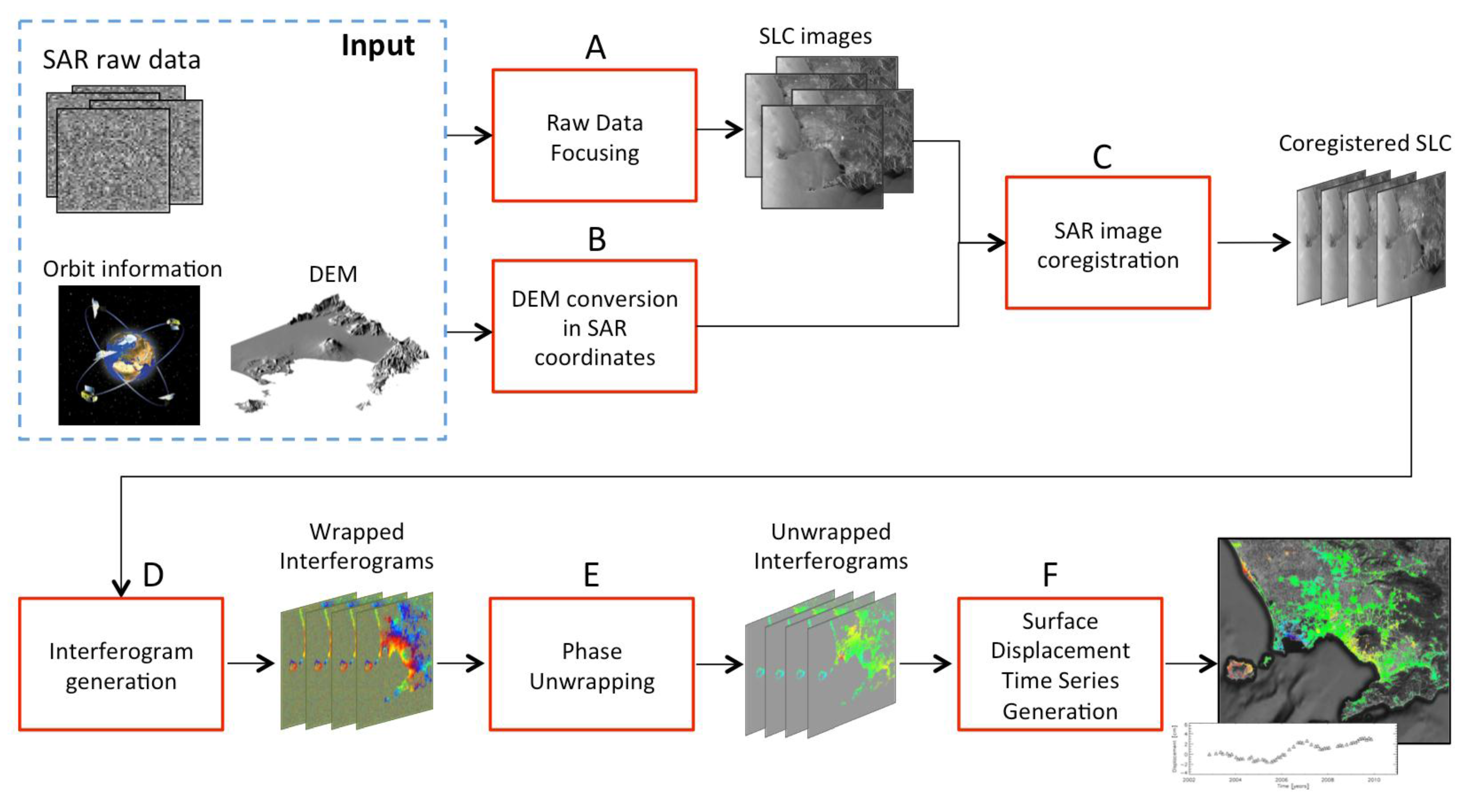
Identify, within the input SAR dataset, data that are acquired at the same epoch but that partially cover the user’s Area of Interest (AoI) and to evaluate the possibility to mosaic them for increasing the investigated area spatial coverage. This feature also permits to automatically discard SAR acquisitions that do not cover the selected AoI. Note that the mosaicking can be performed on adjacent frames of the same track, but not across different tracks;

-

Identify and analyze only the portion of SAR data that cover the AoI, thus reducing the amount of data to be processed and, consequently, the elapsed computing time;

-

Select, among the overall SAR acquisitions, the master image, which is used to identify a reference geometry to minimize the possible error sources during the DInSAR processing. The master image is selected as the closest to the barycenter of the SAR data acquisition distribution in the temporal/perpendicular baseline $\left(T \times b_{\perp }\right)$ plane;

-

Improve the precision of the orbit metadata, e.g., the acquisition start time, by making use of DEM information. Indeed, an incorrect knowledge of the acquisition start time basically translates in a rigid misalignment between the DEM and the SAR acquisitions. To calculate this residual rigid shift, the implemented algorithm first selects an area with high coherence and high phase gradient, within an interferogram less affected by deformation (short temporal baseline) and sensitive to the topography (i.e., with a relatively high perpendicular baseline). Then, it performs a cross-correlation between the phase gradients of the so identified interferogram and the synthetic topography phase computed from the DEM. The peak of the cross-correlation identifies the requested shift;

-

Refine the user-selected reference point of the displacement time series by looking for the one that is affected by the lowest noise level (as defined in [16]) in a surrounding area, thus improving the degree of accuracy of the final DInSAR results. To this aim the algorithm performs, for each interferogram, the phase unwrapping procedure of a patch around the user selected reference point. The point with the higher temporal coherence is then identified as the new reference;

-

Select the pixels to be unwrapped by properly identifying only those that are not significantly affected by noise, thus improving the quality of the final results, taking into account the spatial coherence of each pixels in each data pair;

-

Evaluate the temporal coherence threshold, in dependence of the number of the exploited SAR acquisitions, according to an empirical relationship derived from an extensive analysis of ESA C-band SAR data.

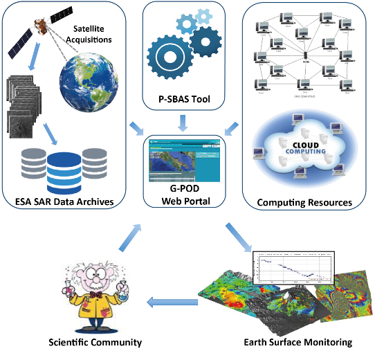
3. G-POD Environment

G-POD is part of the Geohazards Thematic Exploitation Platform (GEP) activity originated by ESA [30]. The GEP, formerly named the Supersites Exploitation Platform (SSEP), was originally specifically designed for Earth Observation (EO) data exploitation in the context of the Geohazard Supersites and Natural Laboratories [31]; however, it has been subsequently expanded in order to address a broader field of objectives concerning the CEOS Pilots on Seismic Hazards and Volcanoes [32].

In particular, G-POD is an environment that was designed by ESA to both orchestrate and manage data processing workflows, in which applications aimed at exploiting EO data can be easily and directly plugged in. More specifically, a generic application can be encapsulated within such a virtual environment and can exploit both distributed high-performance processing resources and large volumes of archived data, in order to provide the scientific community with new EO services [33].

G-POD benefits from the access to the ESA computing facilities as well as to their EO data archives, and provides a friendly web user interface that permits the processing of jobs on a distributed computing system, rather than on PCs or in-house user’s workstations as for traditional applications. This also implies for the final user no installation and update efforts, service access from everywhere (through a web browser) and, at any time, no need to download the input data; last but not least, there is no need to procure and maintain expensive processing hardware. The G-POD environment is, indeed, a complex distributed architecture that is constituted of different logical subsystems, such as computing facility, web portal, services modules repository, and satellite data catalogues.

The computing facility, which is the actual component of the G-POD environment that executes the processing, is composed by several logical elements:

-

A single Computing Element (CE), which acts as a master node in terms of job scheduling policy control;

-

Several Worker Nodes (WNs), which provide the required computation capability;

-

The Storage Elements (SE), where the overall archived data are stored.

The computing resources dedicated to the P-SBAS service are described in Table 1. They are managed by grid and cloud technologies running on Linux operating systems. In addition, a number of utility software such as IDL, Matlab, Sentinel Toolbox, NEST and Gamma are also available [33]. Moreover, thanks to the architecture flexibility, G-POD can easily federate additional computing and storage resources exceeding in this way its base processing capacity. Note also that these G-POD nominal resources belong to ESRIN-ESA but, recently, a new CE has been installed and federated at the IREA-CNR premises [34], which controls 15 WNs (see Table 1) fully dedicated to the P-SBAS service.

Table 1. G-POD resources dedicated to the P-SBAS web tool.

	ESRIN-ESA	IREA-CNR
Worker Nodes	15	15
Virtual CPU	60	30
CPU Type	Intel(R) Xeon(R) X5650 2.67 GHz	Intel(R) Xeon(R) E5-2680 2.70 GHz
RAM /WN	32	64
Storage	2TB	4TB
Network	1 Gbps	1 Gbps

Table 1. G-POD resources dedicated to the P-SBAS web tool.

	ESRIN-ESA	IREA-CNR
Worker Nodes	15	15
Virtual CPU	60	30
CPU Type	Intel(R) Xeon(R) X5650 2.67 GHz	Intel(R) Xeon(R) E5-2680 2.70 GHz
RAM /WN	32	64
Storage	2TB	4TB
Network	1 Gbps	1 Gbps

4. The P-SBAS Web Tool within the G-POD Environment

In this section, we first present the main steps to be accomplished to implement the P-SBAS web tool within the on-demand environment of G-POD; subsequently, the key features and characteristics of the implemented P-SBAS web tool, accessible at [35], are described.

4.1. P-SBAS Web Tool: Implementation

The deployment of the unsupervised P-SBAS algorithm, and in general of a scientific application, within the G-POD environment for developing an on-demand tool accessible via the web requires:

-

A preliminary study of the algorithm aimed at identifying the main independent processes in which it can be decomposed in order to design the proper application workflow;

-

The implementation of the defined workflow in Linux Bash (LB) program language according to the tasks scheduling policy adopted within the G-POD environment. As a result, a set of LB scripts manages the entire P-SBAS algorithm by properly scheduling the different processing steps and, for each parallel step, by correctly distributing the concurrent jobs among the available WNs;

-

The implementation of the LB scripts for executing the processing steps that constitute the P-SBAS workflow and that are launched on the different WNs;

-

The definition and implementation of the web user interface, which allows the configuration and selection of input parameters, thresholds, processing settings, etc.;

-

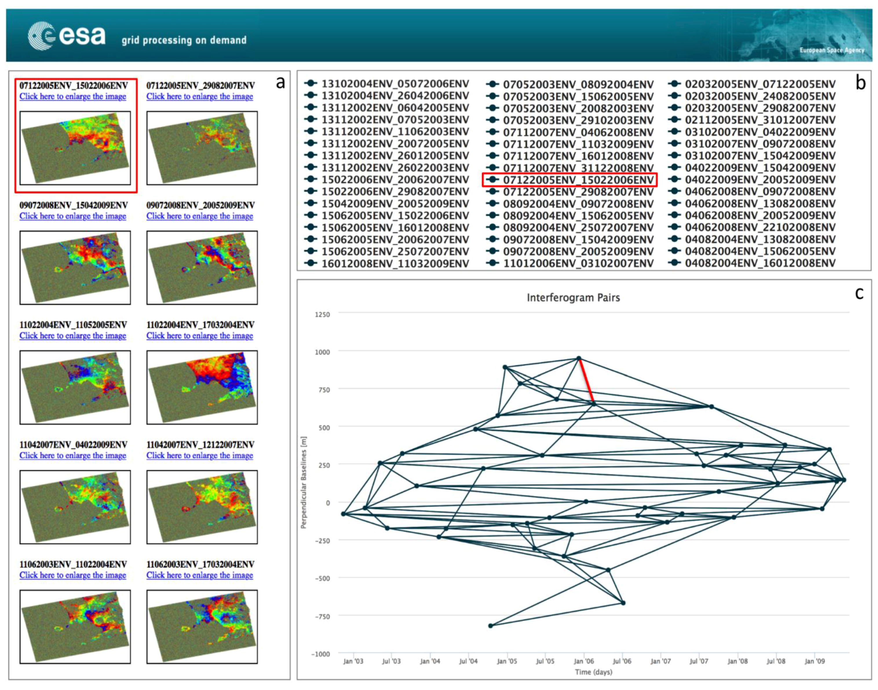
The identification of the whole processing outputs and the implementation of appropriate procedures to collect and make them available for download at the end of the DInSAR processing.

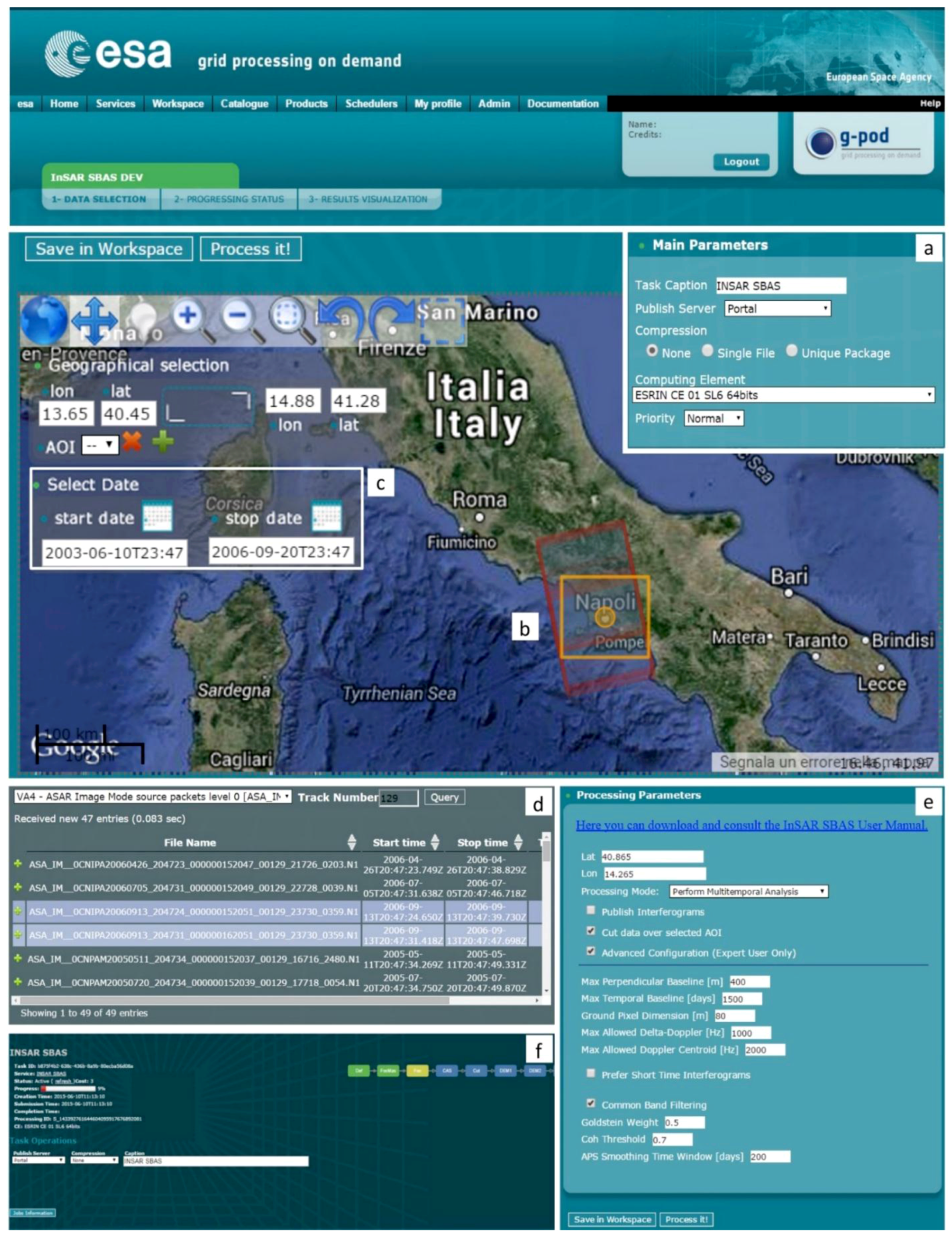
4.2. P-SBAS Web Tool: Features and Characteristics

The access to the developed on-demand P-SBAS web tool on GPOD requires a mandatory registration step on the ESA web portal [36], by creating an ESA Earth Observation Single Sign-On (EO-SSO) account. Then, such an account has to be activated to access the P-SBAS web tool via a request to the Operation Support Team (eo-gpod@esa.int).

Following this preliminary step, the use of the P-SBAS web tool within G-POD is rather straightforward because it simply requires the selection, from the ESA archives, of SAR data to be exploited, and the setting of few parameters needed for the multi-temporal DInSAR processing. The P-SBAS Service is indeed provided with a user-friendly interface, see Figure 2, which allows any user to produce multi-temporal DInSAR products. In particular, the user has to carry out, as only task, the following few actions:

-

Select the computing facilities/resources among those available through the platform, insert the interferometric task caption, select where the final results will be made available to the user, and set the task priority (Figure 2a);

-

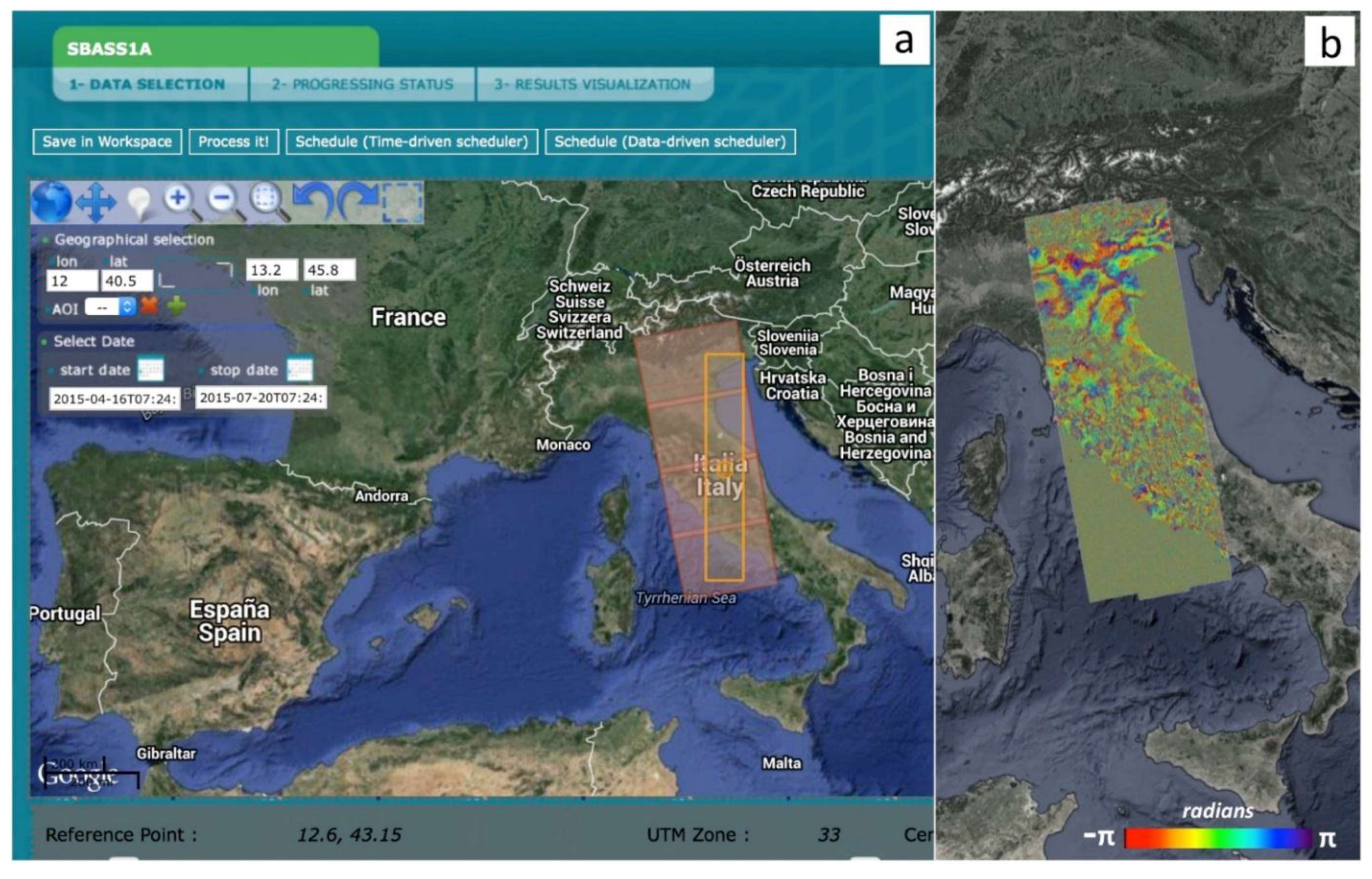
Select the AoI to be processed and the DInSAR reference pixel. The AoI selection is made via a bounding box over an interactive geographical map client (Figure 2b). Instead, the reference point selection is carried out by shifting a place mark over the map client. It is anyway possible to insert geographic coordinates of a known point in the appropriate fields. As a general hint for the reference point selection, it is strongly suggested that it will be located in a stable and (expected) coherent area;

-

Indicate the temporal span used for the subsequent SAR raw data catalogue querying (Figure 2c);

-

Select the ESA data catalogue from which the SAR acquisitions are automatically retrieved. The Virtual Archive 4 (VA4) catalogue [22] is the main source of SAR data for the P-SBAS web tool. VA4 is composed by subsections containing the ENVISAT ASAR and the ERS-1/2 data, the latter being present in both CEOS and ASAR formats. Moreover the possibility to select data by relative orbit number is also provided (Figure 2d);

Figure 2. P-SBAS tool web portal. (a) Main processing Parameters window, (b) geographic map client for the AoI and data selection, (c) investigated time interval selection, (d) SAR data catalogue query, (e) interferometric processing parameters window, and (f) job status monitoring.

Figure 2. P-SBAS tool web portal. (a) Main processing Parameters window, (b) geographic map client for the AoI and data selection, (c) investigated time interval selection, (d) SAR data catalogue query, (e) interferometric processing parameters window, and (f) job status monitoring.

-

Optionally, enter some basic interferometric SAR parameters such as: spatial and temporal baseline thresholds, approximate size (in meters) of the resulting ground pixel, filtering coefficient and noise thresholds (Figure 2e). It is strongly suggested that users skilled on DInSAR processing perform the setting of these parameters. However, to simplify this task for less expert users, default values for each parameter are also provided. It is worth highlighting that these default values are the result of extensive and long-term analyses of ESA C-band data and are suitable for a large part of case studies.

Note that a flag is also available to limit the DInSAR analysis to the generation of multi-temporal interferograms only.

Once the actions above discussed have been performed, the user can start the run of the P-SBAS processing chain on the allocated computing facilities. While running, the user has also the possibility to monitor the process status (Figure 2f) and, once the job is terminated, the final results are available for download from either the G-POD web portal or a user-defined FTP server.

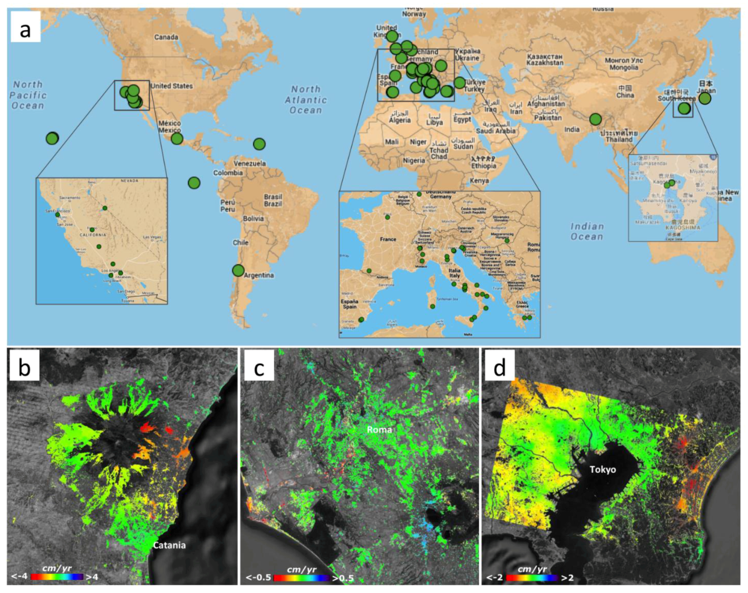
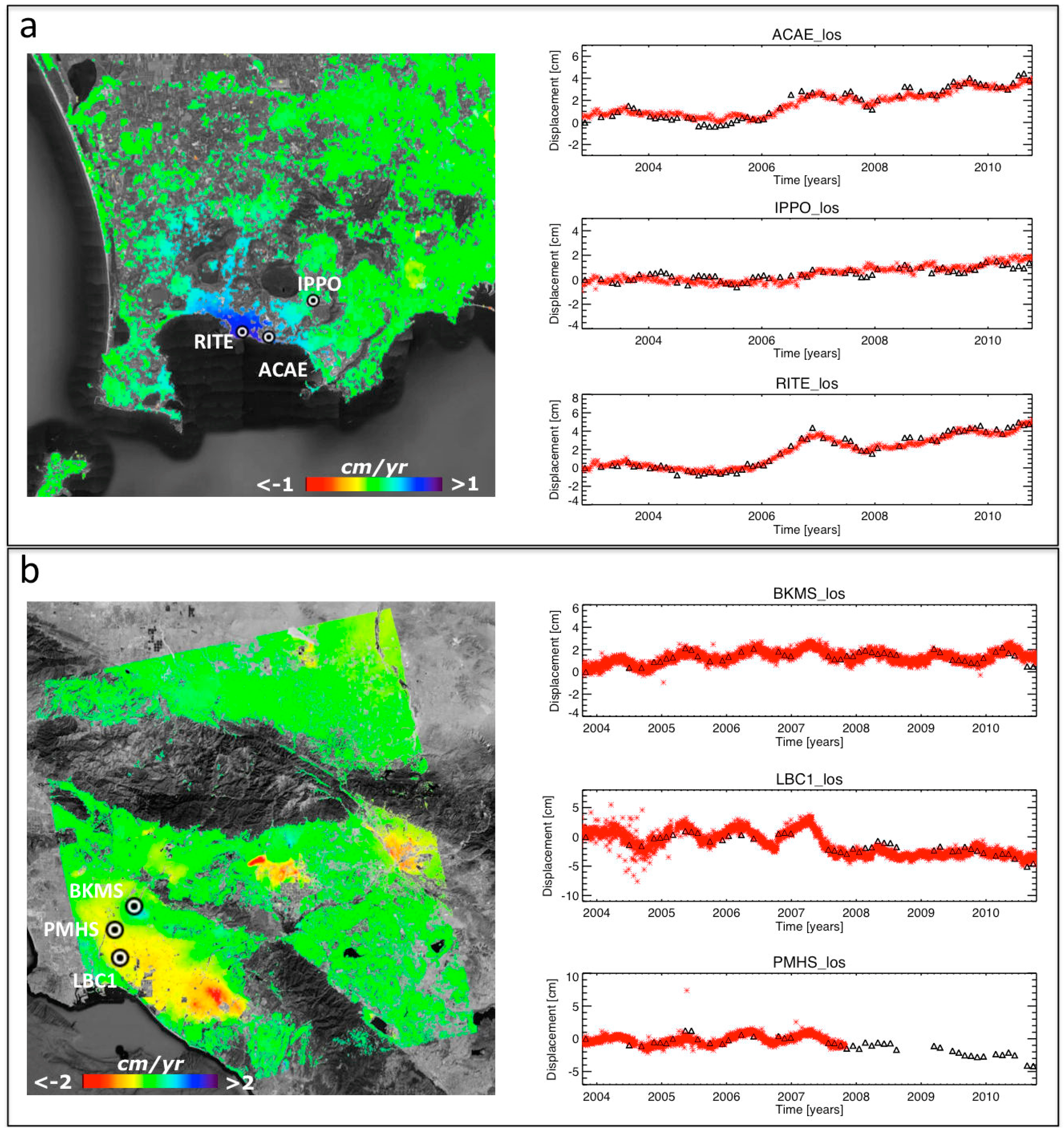
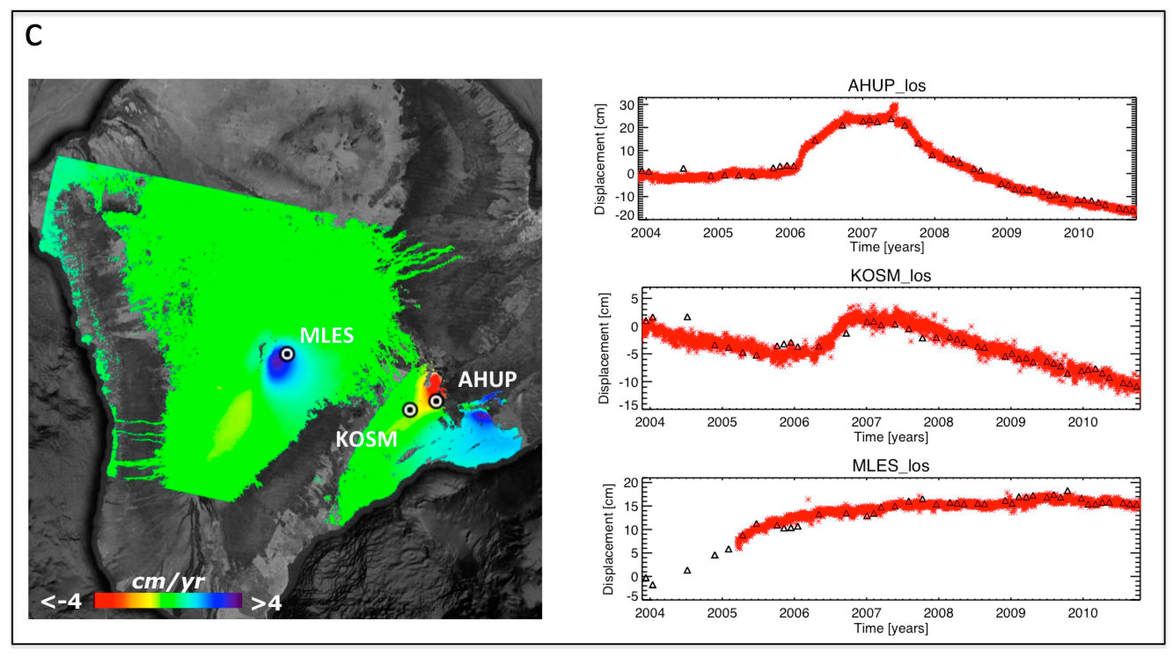
5. Experimental Results

An extensive test and validation activity has been carried out in the six-month period from January to June 2015 in order to assess the performance of the P-SBAS processing chain implemented within the G-POD environment and accessible via the web. To this aim, several datasets, acquired in the 2002–2010 time period by the ENVISAT sensor, have been processed. Figure 3 pictorially shows this intensive P-SBAS service testing activity; moreover, as an example, the computed mean deformation velocity maps relevant to three representative test cases are also shown. In particular, the selected areas are characterized by very heterogeneous behaviours in terms of surface deformation phenomena and interferometric noise sources. Indeed, the Mt. Etna volcano (Figure 3b) is characterized by a complex deformation behavior interested by several eruptions, fault movement and water extraction.

In particular are clearly visible the deformations associated to the activities along the Trecastagni-Mascalucia and Pernicana faults. Figure 3c, instead, presents the displacement map relative to the city of Roma, which is interested by significant subsidence along the Tevere River, due to the compaction of the alluvial deposits.

Finally, in Figure 3d, it is presented the mean deformation velocity map computed over the Tokyo city area, a wide urbanized region affected by subsidence phenomena.

Overall, the whole test and validation activity involved 30 datasets and the achieved results are summarized in Table 2. Note that the exploited datasets consist of SAR data stacks ranging from 15 to 73 acquisitions per area (the average corresponds to 38 SAR acquisitions), which lead to the generation of interferogram sequences spanning the range from 33 to 221 (the average corresponds to 105 interferograms). The spatial extent of each investigated area is of about 100x100 km, which corresponds to about 30000 × 5000 full resolution pixels along azimuth and range directions, respectively. Moreover, a spatial averaging (multilook) of 20 pixels along azimuth and four pixels along range is performed within the interferogram generation step for noise reduction purposes.

The computing resources allocated for each processed dataset consisted in four G-POD working nodes, whose characteristics are described in Table 1. Moreover, it is worth noting that such processing resources can be further expanded whether requested; as a matter of fact, multiple runs can be executed in parallel if needed, by scaling up the selected base infrastructure and plugging-in additional external resources (e.g., cloud computing). According to the exploited G-POD hardware configuration and the investigated SAR datasets, the full P-SBAS processing requires an average time of slightly less than one day (0.94 days), as shown in Table 2.

Figure 3. P-SBAS processing status. (a) Pictorial representation of the processing results achieved by the users through the P-SBAS web tool within G-POD, during the 6-month period January–June 2015, (b), (c), and (d) are the retrieved mean deformation velocity maps relevant to the Mt. Etna (Italy), Roma (Italy) and Tokyo (Japan) areas, respectively.

Figure 3. P-SBAS processing status. (a) Pictorial representation of the processing results achieved by the users through the P-SBAS web tool within G-POD, during the 6-month period January–June 2015, (b), (c), and (d) are the retrieved mean deformation velocity maps relevant to the Mt. Etna (Italy), Roma (Italy) and Tokyo (Japan) areas, respectively.

In addition it is worth remarking that the implemented unsupervised P-SBAS solution does not significantly affect the quality of the retrieved DInSAR results, in terms of the accuracies of the retrieved measurements. To verify this issue we have compared the achieved P-SBAS results with those obtained through GPS measurements. We present in the following the results relevant to the ENVISAT datasets available over three test sites: the Campi Flegrei caldera (Italy), the Los Angeles area (US) and the Mauna Loa and Kilauea volcanoes in Hawaii (US). These areas are interested by different deformation behaviors; indeed, the Campi Flegrei is a well-known active volcanic zone close to the Napoli city (Italy), which is experiencing an almost continuous uplift of the Earth surface since late 2004 [37]. Los Angeles is a wide urbanized region affected by oil extraction, aquifer exploitation (implying periodic displacements) and seismic activity [38]. Finally, Hawaii volcanoes are among the most active in the world, as testified by the frequent unrest episodes and eruptions [39] and thus implying a strongly non-linear deformation behavior of the ground.

Table 2. ENVISAT SAR data sets processed through the P-SBAS web tool during the 6-month testing period January-June 2015.

Site *	Images	Interf	Coherent Pixels	Elapsed Time (day)
Tokyo	29	86	407600	0.66
Los Angeles	44	127	661614	1.46
Hawaii_471	37	106	1105564	1.41
Hawaii_200	42	123	446053	0.87
Hawaii_408	36	105	544544	0.80
Hawaii_343	20	50	405365	0.52
Hawaii_136	15	34	448017	0.50
Hawaii_114	19	33	681393	0.44
S. Francisco	43	126	282653	0.92
Galápagos	63	187	617029	2.11
London	49	138	282496	0.87
Homs_307	34	93	288442	0.60
Homs_78	33	94	136727	0.54
Long Valley	50	131	619025	1.99
Roma	39	112	126059	0.62
Ferrara	20	51	113850	0.74
Paris	50	148	253886	1.02
Atene	44	76	124758	0.48
Amsterdam	73	221	143743	1.13
Messico City	50	140	284014	0.97
Racconigi	34	92	157682	0.96
Napoli_36	57	168	119159	0.85
Fresno	32	91	193371	0.63
Lorca	27	75	576065	1.48
Sacramento	42	118	130383	0.89
Copahue_261	31	92	133150	0.47
Atacama	18	46	1645812	1.24
Turkey	29	81	115342	0.71
Delano	34	98	193977	1.48
Average	38.03	104.89	387509.41	0.94

* Note that the site names have been defined by the users.

Table 2. ENVISAT SAR data sets processed through the P-SBAS web tool during the 6-month testing period January-June 2015.

Site *	Images	Interf	Coherent Pixels	Elapsed Time (day)
Tokyo	29	86	407600	0.66
Los Angeles	44	127	661614	1.46
Hawaii_471	37	106	1105564	1.41
Hawaii_200	42	123	446053	0.87
Hawaii_408	36	105	544544	0.80
Hawaii_343	20	50	405365	0.52
Hawaii_136	15	34	448017	0.50
Hawaii_114	19	33	681393	0.44
S. Francisco	43	126	282653	0.92
Galápagos	63	187	617029	2.11
London	49	138	282496	0.87
Homs_307	34	93	288442	0.60
Homs_78	33	94	136727	0.54
Long Valley	50	131	619025	1.99
Roma	39	112	126059	0.62
Ferrara	20	51	113850	0.74
Paris	50	148	253886	1.02
Atene	44	76	124758	0.48
Amsterdam	73	221	143743	1.13
Messico City	50	140	284014	0.97
Racconigi	34	92	157682	0.96
Napoli_36	57	168	119159	0.85
Fresno	32	91	193371	0.63
Lorca	27	75	576065	1.48
Sacramento	42	118	130383	0.89
Copahue_261	31	92	133150	0.47
Atacama	18	46	1645812	1.24
Turkey	29	81	115342	0.71
Delano	34	98	193977	1.48
Average	38.03	104.89	387509.41	0.94

* Note that the site names have been defined by the users.

Exploited ENVISAT datasets span the 2003–2010 time interval and are composed by 65 (Track 129), 45 (Track 120) and 42 (Track 200) ASAR data for the Campi Flegrei, Los Angeles and Hawaii sites, respectively. Moreover, extended GPS networks have been installed in all the three selected sites. In particular, the Campi Flegrei network is active since 2000 [40], the Los Angeles one has been completed in 2001 [41], while the first GPS station on Hawaii was activated in 1995 [42].

Within the selected test sites, the GPS measurements have been compared with those obtained through the unsupervised P-SBAS processing. In particular, among several, we identified 100 stations that are both located in correspondence with coherent pixels and guarantee a temporal overlap with the P-SBAS measurements of at least two years. Moreover, since we considered the GPS as our reference, we neglected the stations highly affected by noise (i.e., spikes or average of nominal sigma values larger than 4 mm in LOS). As an example, in Figure 4, we show the surface deformation mean velocity map retrieved for the three test sites with highlighted, per each of them, the positions of three representative GPS stations; for the same stations, the displacement time series retrieved by both the GPS measurements and the P-SBAS processing are depicted as well. Plots of Figure 4 permit us also to show the capability of the unsupervised P-SBAS algorithm to correctly detect and follow complex deformation behavior characterized by periodic signals and strong non-linearity.

Figure 4. Unsupervised P-SBAS processing chain validation experiments. Per each of the three selected test sites are shown: the mean deformation velocity maps retrieved from the P-SBAS analysis; the locations of three selected GPS stations; the comparison between the GPS (red stars) and the P-SBAS (black triangles) surface deformation time series relevant to the stations identified in the corresponding map; the standard deviations ($\text{σ}$) of the difference between the GPS and the DInSAR measurements. (a) Campi Flegrei caldera. (b) Los Angeles. (c) Hawaii.

Figure 4. Unsupervised P-SBAS processing chain validation experiments. Per each of the three selected test sites are shown: the mean deformation velocity maps retrieved from the P-SBAS analysis; the locations of three selected GPS stations; the comparison between the GPS (red stars) and the P-SBAS (black triangles) surface deformation time series relevant to the stations identified in the corresponding map; the standard deviations ($\text{σ}$) of the difference between the GPS and the DInSAR measurements. (a) Campi Flegrei caldera. (b) Los Angeles. (c) Hawaii.

For all the 100 selected stations we calculated the standard deviation of the difference between the P-SBAS and GPS time series, obtaining average values of about 4.0 mm, 6.6 mm and 11.8 mm for the Campi Flegrei, Los Angeles and Hawaii sites, respectively (see Table 3). Note that, even if in this case it is assumed as the reference, the GPS measurements are themselves affected by noise. Therefore, per each station of for the three test sites, we empirically estimated the standard deviations of the GPS time series with respect to a smoothed version of the time series itself, in the time period common to the SAR acquisitions. Obtained values are about 1 mm, 3 mm and 6 mm, for the Campi Flegrei, Los Angeles and Hawaii test sites, respectively. By considering these values, we may remove from the P-SBAS/GPS time series standard deviations the bias due to the estimated errors relevant to the geodetic measurements.

The achieved results very well match with the expected SBAS technique accuracy [23]. Accordingly, these validation experiments confirm the good agreement between the conventional SBAS and the unsupervised P-SBAS versions, demonstrating that the latter preserves the accuracies of the SBAS results.

Table 3. Results of the comparison between SAR and LOS-projected GPS deformation time series.

Test Site	GPS Station	Standard Deviation of the Difference between SAR and LOS-Projected GPS Measurements (cm)	Test Site	GPS Station	Standard Deviation of the Difference between SAR and LOS-Projected GPS Measurements (cm)
Campi Flegrei	ACAE	0.42	Hawaii	AHUP	1.41
	ARFE	0.33		AINP	0.90
	BAIA	0.41		ALAL	0.84
	FRUL	0.38		ALEP	1.13
	IPPO	0.40		ANIP	0.72
	LICO	0.41		BLBP	1.15
	MORU	0.41		BYRL	1.95
	QUAR	0.35		CNPK	0.51
	RITE	0.37		CRIM	0.82
	STRZ	0.31		ELEP	0.95
Los Angeles	BGIS	0.57		GOPM	1.49
	BILL	0.56		HOLE	1.69
	BKMS	0.92		KAEP	2.12
	CHIL	0.52		KAMO	1.23
	CIT1	1.06		KFAP	0.73
	CJMS	0.69		KHKU	0.88
	CLAR	1.24		KNNE	0.73
	CSDH	0.54		KOSM	1.21
	CVHS	0.86		KTPM	1.64
	DVPB	0.70		MANE	1.13
	EWPP	0.65		MLCC	0.90
	GHRP	1.01		MLES	0.90
	HOLP	0.56		MLPR	0.55
	LBC1	0.57		MLRD	0.88
	LBC2	0.54		MLSP	1.25
	LBCH	0.56		MOKP	2.16
	LL01	0.70		NPIT	0.95
	LORS	0.34		OUTL	0.69
	MAT2	0.53		PGF1	1.65
	MLFP	0.66		PGF2	2.13
	MTA1	0.79		PGF3	1.74
	NOCO	0.51		PGF4	1.71
	OXYC	0.57		PGF5	1.80
	P470	0.75		PGF6	1.74
	P471	0.50		PHAN	0.74
	P476	0.84		PIIK	0.88
	P477	0.83		PMAU	1.15
	P577	1.13		PUKA	0.86
	P581	0.51		RADF	0.86
	P586	0.56		SLPC	0.82
	P587	0.48		STEP	1.11
	P612	0.59		TOUO	1.30
	PBPP	0.48		UWEV	0.98
	PMHS	0.32		YEEP	0.85
	PPBF	0.63
	RHCL	0.52
	SBCC	0.62
	SGHS	0.77
	SILK	0.64
	SPMS	0.37
	USC1	0.28
	VDCY	0.57
	VYAS	0.56
	WCHS	0.92
	WHC1	0.52
	WNRA	1.06

Table 3. Results of the comparison between SAR and LOS-projected GPS deformation time series.

Test Site	GPS Station	Standard Deviation of the Difference between SAR and LOS-Projected GPS Measurements (cm)	Test Site	GPS Station	Standard Deviation of the Difference between SAR and LOS-Projected GPS Measurements (cm)
Campi Flegrei	ACAE	0.42	Hawaii	AHUP	1.41
	ARFE	0.33		AINP	0.90
	BAIA	0.41		ALAL	0.84
	FRUL	0.38		ALEP	1.13
	IPPO	0.40		ANIP	0.72
	LICO	0.41		BLBP	1.15
	MORU	0.41		BYRL	1.95
	QUAR	0.35		CNPK	0.51
	RITE	0.37		CRIM	0.82
	STRZ	0.31		ELEP	0.95
Los Angeles	BGIS	0.57		GOPM	1.49
	BILL	0.56		HOLE	1.69
	BKMS	0.92		KAEP	2.12
	CHIL	0.52		KAMO	1.23
	CIT1	1.06		KFAP	0.73
	CJMS	0.69		KHKU	0.88
	CLAR	1.24		KNNE	0.73
	CSDH	0.54		KOSM	1.21
	CVHS	0.86		KTPM	1.64
	DVPB	0.70		MANE	1.13
	EWPP	0.65		MLCC	0.90
	GHRP	1.01		MLES	0.90
	HOLP	0.56		MLPR	0.55
	LBC1	0.57		MLRD	0.88
	LBC2	0.54		MLSP	1.25
	LBCH	0.56		MOKP	2.16
	LL01	0.70		NPIT	0.95
	LORS	0.34		OUTL	0.69
	MAT2	0.53		PGF1	1.65
	MLFP	0.66		PGF2	2.13
	MTA1	0.79		PGF3	1.74
	NOCO	0.51		PGF4	1.71
	OXYC	0.57		PGF5	1.80
	P470	0.75		PGF6	1.74
	P471	0.50		PHAN	0.74
	P476	0.84		PIIK	0.88
	P477	0.83		PMAU	1.15
	P577	1.13		PUKA	0.86
	P581	0.51		RADF	0.86
	P586	0.56		SLPC	0.82
	P587	0.48		STEP	1.11
	P612	0.59		TOUO	1.30
	PBPP	0.48		UWEV	0.98
	PMHS	0.32		YEEP	0.85
	PPBF	0.63
	RHCL	0.52
	SBCC	0.62
	SGHS	0.77
	SILK	0.64
	SPMS	0.37
	USC1	0.28
	VDCY	0.57
	VYAS	0.56
	WCHS	0.92
	WHC1	0.52
	WNRA	1.06

We finally note that, even if the accuracy of the retrieved measurement is fully preserved by the unsupervised P-SBAS web tool, it is possible that supervised processing could perform better in terms of the final number of measure points, due to an ad hoc selection of the involved interferograms.

6. Further Developments

As already mentioned, the presented P-SBAS web tool has been designed to generate DInSAR products in an unsupervised way, thus reducing the user interaction to only few initial steps. This permits to attract users who are not expert or not interested on DInSAR processing, with the final aim to extend the scientific community involved in DInSAR analysis.

Figure 5. Web interface for the interferograms selection. (a) Quick looks of the inteferograms generated by the P-SBAS web tool (the example is relevant to the ENVISAT data over Napoli Bay area, see Figure 2). One selected interferogram is highlighted via red square, (b) List of the interferometric pairs with, highlighted, the same interferogram considered in Figure 5a, and (c) distribution of the interferometric pairs in the temporal (x-axis) vs. spatial baseline (y-axis) plane. Additionally, in this case the same interferogram considered in Figure 5a is highlighted.

Figure 5. Web interface for the interferograms selection. (a) Quick looks of the inteferograms generated by the P-SBAS web tool (the example is relevant to the ENVISAT data over Napoli Bay area, see Figure 2). One selected interferogram is highlighted via red square, (b) List of the interferometric pairs with, highlighted, the same interferogram considered in Figure 5a, and (c) distribution of the interferometric pairs in the temporal (x-axis) vs. spatial baseline (y-axis) plane. Additionally, in this case the same interferogram considered in Figure 5a is highlighted.

However, the followed approach does not allow to analysis of the intermediate results (e.g., the interferograms) and it does not permit carrying out any fine tuning of processing parameters, depending on the characteristics of the considered SAR dataset and investigated area. This clearly limits the possibility to customize the DInSAR processing and make the developed web tool less attractive for expert DInSAR users. To relax such constraints, a future release of our web tool, which is already under testing and is planned to be open by the end of 2015, will provide the user with the possibility to increase his interaction with the processing. In particular, following the interferogram generation step (Block D in Figure 1), it will be allowed to visually check the generated interferograms and to interactively discard those that present a high level of noise, thus permitting to further increase the density of the investigated coherent pixels. Figure 5 shows the web interface that allows performing the described interferogram selection process.

It is also worth noting that the implemented P-SBAS web tool is currently able to process ESA’s ERS and ENVISAT data, but it is designed to deal also with COSMO-SkyMed (Italy), TerraSAR-X (Germany), ALOS-1/2 (Japan), RADARSAT-1/2 (Canada) acquired in Stripmap mode. Moreover, an upcoming release will permit to further expand the presented P-SBAS web tool to process the forthcoming huge SAR data archive acquired by the Sentinel-1 mission [43]; in this case the implementation phase is smoothly moving forward and some first results are already available (see Figure 6).

Figure 6. Sentinel-1 first results. (a) G-POD web interface relevant to the P-SBAS tool for DInSAR analysis of Sentinel-1 data, and (b) example of an interferogram generated through the P-SBAS tool in an unsupervised way, by exploiting a Sentinel-1 interferometric pair obtained merging four slices per each acquisition. Contains Copernicus data ©2015.

Figure 6. Sentinel-1 first results. (a) G-POD web interface relevant to the P-SBAS tool for DInSAR analysis of Sentinel-1 data, and (b) example of an interferogram generated through the P-SBAS tool in an unsupervised way, by exploiting a Sentinel-1 interferometric pair obtained merging four slices per each acquisition. Contains Copernicus data ©2015.

We remark the relevance of these Sentinel-1 data, characterized by a reduced revisit time (6 days when both Sentinel-1A and Sentinel-1B will be operative in 2016), a very large spatial coverage and a free and open access data policy, which will open new challenging perspectives to the comprehension of the Earth surface deformation dynamics at very extended spatial scales.

Finally, we stress that the present release of the web tool deals with three-arcsec DEM freely available from the SRTM archive. In future releases, we will plan to also exploit the one-arcsec version of the SRTM as well as we investigate the technical possibility for users to upload their own generated DEM.

7. Conclusions

In this paper we presented an on-demand and unsupervised web tool for the generation of DInSAR deformation time series and mean deformation velocity map. The motivation for the development of such a tool comes from the idea of moving both DInSAR algorithms and computational resources close to SAR data in order to pursue the full exploitation of the existing (and forthcoming) archives. In particular, an operational DInSAR processing chain, accessible through the web, has been set up to process ESA SAR data by properly exploiting (a) the P-SBAS multi-temporal DInSAR algorithm, (b) the high-performance and sizeable computing resources provided by the G-POD environment, and (c) the directly accessible ESA archives. Accordingly, the implemented tool lets the users free from the necessity of ordering and downloading SAR data, as well as of procuring a DInSAR processing algorithm and the needed computing resources.

The proposed solution allows the provisioning of a fully-unsupervised P-SBAS processing service to non-expert users, as well as to expert ones that can benefit from a tool that permit a fast exploration of a study area and a better control of the processing chain (e.g., through the interactive interferogram selection), thus expanding the access to high quality multi-temporal DInSAR results. Such a service provides the users not only with a fully-functional on-demand P-SBAS web tool but also with a technical and scientific support for either addressing possible issues or suggesting optimal usage. Such a support can be obtained through the dedicated G-POD team (eo-gpod@esa.int); moreover, a detailed user manual is also available for download [44] to allow users to exploit the tool as easily as possible. Furthermore, the flexibility of the exploited G-POD architecture makes simple to federate additional computing and storage resources which can be also provided through cloud environments. Indeed, conjugating this approach with cloud computing infrastructures is foreseen because it will permit to avoid possible bottlenecks, represented by the intrinsic limited resources of in-house facilities [27], and to extend this service to a wider number of users.

In addition, the availability of this and other web tools within the ESA’s GEP initiative, will allow users to remotely process the data, as well as to share, promote, and discover the obtained results among the platform community, thus fostering the creation of an environment where doing science in a new way.

Finally, it is worth remarking the coming possibility, by the end of 2015, to dispose of a similar web tool able to process Sentinel-1 TOPS data, thus allowing users to generate DInSAR results at theoretically worldwide scale.

References

- Massonnet, D.; Feigl, K.L. Radar interferometry and its application to changes in the Earth’s surface. Rev. Geophys. 1998, 36, 441–500. [Google Scholar] [CrossRef]
- Burgmann, R.; Rosen, P.A.; Fielding, E.J. Synthetic aperture radar interferometry to measure Earth’s surface topography and its deformation. Ann. Rev. Earth Planet. Sci. 2000, 28, 169–209. [Google Scholar] [CrossRef]
- Gabriel, A.K.; Goldstein, R.M.; Zebker, H.A. Mapping small elevation changes over large areas: Differential interferometry. J. Geophys. Res. 1989, 94, 9183–9191. [Google Scholar] [CrossRef]
- Franceschetti, G.; Lanari, R. Synthetic Aperture Radar Processing; CRC Press: Boca Raton, FL, USA, 1999. [Google Scholar]
- Massonnet, D.; Rossi, M.; Carmona, C.; Adragna, F.; Peltzer, G.; Feigl, K.; Rabaute, T. The displacement field of the Landers earthquake mapped by radar interferometry. Nature 1993, 364, 138–142. [Google Scholar] [CrossRef]
- Ferretti, A.; Prati, C.; Rocca, F. Permanent scatterers in SAR interferometry. IEEE Trans. Geosci. Remote Sens. 2001, 39, 8–20. [Google Scholar] [CrossRef]
- Werner, C.; Wegmüller, U.; Strozzi, T.; Wiesmann, A. Interferometric point target analysis for deformation mapping. In Proceedings of the Geoscience and Remote Sensing Symposium, Toulouse, France, 21–25 July 2003; pp. 4362–4364.
- Hooper, A.; Zebker, H.; Segall, P.; Kampes, B. A new method for measuring deformation on volcanoes and other natural terrains using InSAR persistent scatterers. Geophys. Res. Lett. 2004, 31, L23611. [Google Scholar] [CrossRef]
- Kampes, B.M. Radar Interferometry: Persistent Scatterer Technique; Springer-Verlag: Dordrecht, The Netherlands, 2006. [Google Scholar]
- Berardino, P.; Fornaro, G.; Lanari, R.; Sansosti, E. A new algorithm for surface deformation monitoring based on small baseline differential SAR interferograms. IEEE Trans. Geosci. Remote Sens. 2002, 40, 2375–2383. [Google Scholar] [CrossRef]
- Mora, O.; Mallorquí, J.J.; Broquetas, A. Linear and nonlinear terrain deformation maps from a reduced set of interferometric SAR images. IEEE Trans. Geosci. Remote Sens. 2003, 41, 2243–2253. [Google Scholar] [CrossRef]
- Crosetto, M.; Crippa, B.; Biescas, E. Early detection and in-depth analysis of deformation phenomena by radar interferometry. Eng. Geol. 2005, 79, 81–91. [Google Scholar] [CrossRef]
- Sansosti, E.; Casu, F.; Manzo, M.; Lanari, R. Space-borne radar interferometry techniques for the generation of deformation time series: An advanced tool for Earth’s surface displacement analysis. Geophys. Res. Lett. 2010, 37, L20305. [Google Scholar] [CrossRef]
- Lanari, R.; Mora, O.; Manunta, M.; Mallorquí, J.J.; Berardino, P.; Sansosti, E. A small-baseline approach for investigating deformations on full-resolution differential SAR interferograms. Int. IEEE Trans. Geosci. Remote Sens. 2004, 42, 1377–1386. [Google Scholar] [CrossRef]
- Strang, G. Linear Algebra and Its Applications; Harcourt Brace Jovanovich: Orlando, FL, USA, 1988. [Google Scholar]
- Zebker, H.A.; Villasenor, J. Decorrelation in interferometric radar echoes. IEEE Trans. Geosci. Remote Sens. 1992, 30, 950–959. [Google Scholar] [CrossRef]
- Casu, F.; Elefante, S.; Imperatore, P.; Zinno, I.; Manunta, M.; De Luca, C.; Lanari, R. SBAS-DInSAR parallel processing for deformation time-series computation. IEEE J. Sel. Top. Appl. Earth Obs. Remote Sens. 2014, 7, 3285–3296. [Google Scholar] [CrossRef]
- Zinno, I.; Mossucca, L.; Elefante, S.; Luca, C.; Casola, V.; Terzo, O.; Casu, F.; Lanari, R. Cloud computing for earth surface deformation analysis via spaceborne radar imaging: A case study. IEEE Trans. Cloud Comput. 2015, 99. [Google Scholar] [CrossRef]
- Rosen, P.A.; Hensley, S.; Peltzer, G.; Simons, M. Updated repeat orbit interferometry package released. EOS Trans. Am. Geophys. Union 2004, 85, 47. [Google Scholar] [CrossRef]
- Agram, P.S.; Jolivet, R.; Riel, B.; Lin, Y.N.; Simons, M.; Hetland, E.; Doin, M.P.; Lassere, C. New radar interferometric time series analysis toolbox released. Eos Trans. AGU 2013, 94, 69–70. [Google Scholar] [CrossRef]
- Marchetti, P.G.; Rivolta, G.; D’elia, S.; Farres, J.; Gobron, N.; Mason, G. A Model for the Scientific Exploitation of Earth Observation Missions: The ESA Research and Service Support. IEEE Geosci. Newsl. 2012, 162, 10–18. [Google Scholar]
- Virtual Archive 4. Available online: http://eo-virtual-archive4.esa.int/ (accessed on 9 September 2015).
- Lanari, R.; Casu, F.; Manzo, M.; Zeni, G.; Berardino, P.; Manunta, M.; Pepe, A. An overview of the small baseline subset algorithm: A DInSAR technique for surface deformation analysis. Pure Appl. Geophys. 2007, 164, 637–661. [Google Scholar] [CrossRef]
- Casu, F.; Manzo, M.; Lanari, R. A quantitative assessment of the SBAS algorithm performance for surface deformation retrieval from DInSAR data. Remote Sens. Environ. 2006, 102, 195–210. [Google Scholar] [CrossRef]
- Manzo, M.; Fialko, Y.; Casu, F.; Pepe, A.; Lanari, R. A quantitative assessment of DInSAR measurements of interseismic deformation: The southern San Andreas Fault case study. Pure Appl. Geophys. 2012, 169, 1463–1482. [Google Scholar] [CrossRef]
- Bonano, M.; Manunta, M.; Pepe, A.; Paglia, L.; Lanari, R. From previous C-band to new X-band SAR systems: Assessment of the DInSAR mapping improvement for deformation time-series retrieval in urban areas. IEEE Trans. Geosci. Remote Sens. 2013, 51, 1973–1984. [Google Scholar] [CrossRef]
- Lanari, R.; Casu, F.; Manzo, M.; Lundgren, P. Application of the SBAS-DInSAR technique to fault creep: A case study of the Hayward fault, California. Remote Sens. Environ. 2007, 109, 20–28. [Google Scholar] [CrossRef]
- Goldstein, R.M. Atmospheric limitations to repeat-track radar interferometry. Geophys. Res. Lett. 1995, 22, 2517–2520. [Google Scholar] [CrossRef]
- Pepe, A.; Lanari, R. On the extension of the minimum cost flow algorithm for phase unwrapping of multitemporal differential SAR interferograms. IEEE Trans. Geosci. Remote Sens. 2006, 44, 2374–2383. [Google Scholar] [CrossRef]
- Geohazard Exploitation Platform. Available online: https://geohazards-tep.eo.esa.int/#! (accessed on 9 September 2015).
- Geohazard Supersites and Natural Laboratories. Available online: http://supersites.earthobservations.org (accessed on 9 September 2015).
- CEOS. Available online: http://www.ceos.org/index.php?option=com_content&view=category&layout=blog&id=355&Itemid=491 (accessed on 9 September 2015).
- GRID Processing on Demand. Available online: http://wiki.services.eoportal.org/tiki-index.php?page=GPOD%20Wiki (accessed on 9 September 2015).
- IREA. Available online: http://www.irea.cnr.it/en/index.php (accessed on 9 September 2015).
- G-POD. Available online only for registered users: http://gpod.eo.esa.int/services/SBAS (accessed on 30 October 2015).
- European Space Agency. Available online: https://earth.esa.int/web/guest/missions/esa-operational-eo-missions (accessed on 9 September 2015).
- Trasatti, E.; Casu, F.; Giunchi, C.; Pepe, S.; Solaro, G.; Tagliaventi, S.; Berardino, P.; Manzo, M.; Pepe, A.; Ricciardi, G.P.; et al. The 2004–2006 uplift episode at Campi Flegrei caldera (Italy): Constraints from SBAS-DInSAR ENVISAT data and Bayesian source inference. Geophys. Res. Lett. 2008, 35, L073078. [Google Scholar] [CrossRef]
- Lanari, R.; Lundgren, P.; Manzo, M.; Casu, F. Satellite radar interferometry time series analysis of surface deformation for Los Angeles, California. Geophys. Res. Lett. 2004, 31, L23613. [Google Scholar] [CrossRef]
- Poland, M.P.; Sutton, A.J.; Gerlach, T.M. Magma degassing triggered by static decompression at Kīlauea Volcano, Hawaii. Geophys. Res. Lett. 2009, 36, L16306. [Google Scholar] [CrossRef]
- De Martino, P.; Tammaro, U.; Obrizzo, F. GPS time series at Campi Flegrei caldera (2000–2013). Ann. Geophys. 2014, 57, S0213. [Google Scholar]
- SCIGN. Available online: http://www.scign.com (accessed on 30 October 2015).
- UNAVCO. Available online: http://www.unavco.org/data/gps-gnss/data-access-methods/dai2/app/dai2.html#scope=All;boundingBox=16.4296,-162.2705,23.2049,-151.7236 (accessed on 10 November 2015).
- ESA-Sentinel. Available online: https://sentinel.esa.int/web/sentinel/home (accessed on 10 November 2015).
- P-SBAS Manual. Available online: https://wiki.services.eoportal.org/tiki-download_file.php?fileId=883 (accessed on 9 September 2015).
© 2015 by the authors; licensee MDPI, Basel, Switzerland. This article is an open access article distributed under the terms and conditions of the Creative Commons Attribution license (http://creativecommons.org/licenses/by/4.0/).
Share and Cite
De Luca, C.; Cuccu, R.; Elefante, S.; Zinno, I.; Manunta, M.; Casola, V.; Rivolta, G.; Lanari, R.; Casu, F. An On-Demand Web Tool for the Unsupervised Retrieval of Earth’s Surface Deformation from SAR Data: The P-SBAS Service within the ESA G-POD Environment. Remote Sens. 2015, 7, 15630-15650. https://doi.org/10.3390/rs71115630
De Luca C, Cuccu R, Elefante S, Zinno I, Manunta M, Casola V, Rivolta G, Lanari R, Casu F. An On-Demand Web Tool for the Unsupervised Retrieval of Earth’s Surface Deformation from SAR Data: The P-SBAS Service within the ESA G-POD Environment. Remote Sensing. 2015; 7(11):15630-15650. https://doi.org/10.3390/rs71115630
Chicago/Turabian StyleDe Luca, Claudio, Roberto Cuccu, Stefano Elefante, Ivana Zinno, Michele Manunta, Valentina Casola, Giancarlo Rivolta, Riccardo Lanari, and Francesco Casu. 2015. "An On-Demand Web Tool for the Unsupervised Retrieval of Earth’s Surface Deformation from SAR Data: The P-SBAS Service within the ESA G-POD Environment" Remote Sensing 7, no. 11: 15630-15650. https://doi.org/10.3390/rs71115630
APA StyleDe Luca, C., Cuccu, R., Elefante, S., Zinno, I., Manunta, M., Casola, V., Rivolta, G., Lanari, R., & Casu, F. (2015). An On-Demand Web Tool for the Unsupervised Retrieval of Earth’s Surface Deformation from SAR Data: The P-SBAS Service within the ESA G-POD Environment. Remote Sensing, 7(11), 15630-15650. https://doi.org/10.3390/rs71115630