
Frequency of Low Clouds in Taiwan Retrieved from MODIS Data and Its Relation to Cloud Forest Occurrence

Abstract
:
1. Introduction
2. Material and Methods
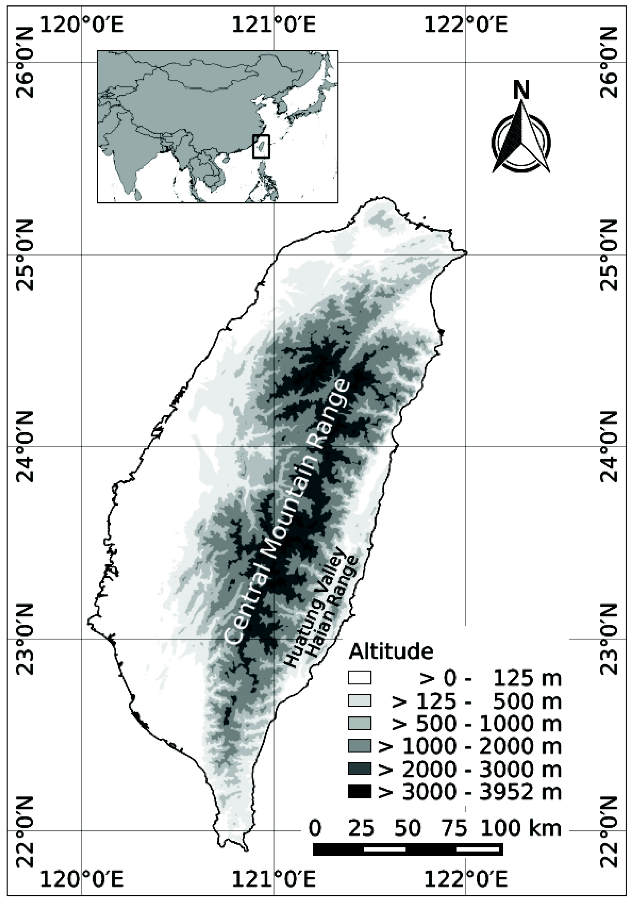
2.1. Study Area

2.2. Data
2.2.1. MODIS Cloud Mask
- Terra overflight: ca. 2:00 am–3:30 am UTC, 10:00 am–11:30 am local time
- Aqua overflight: ca. 4:30 am–6:00 am UTC, 12:30 pm–2:00 pm local time
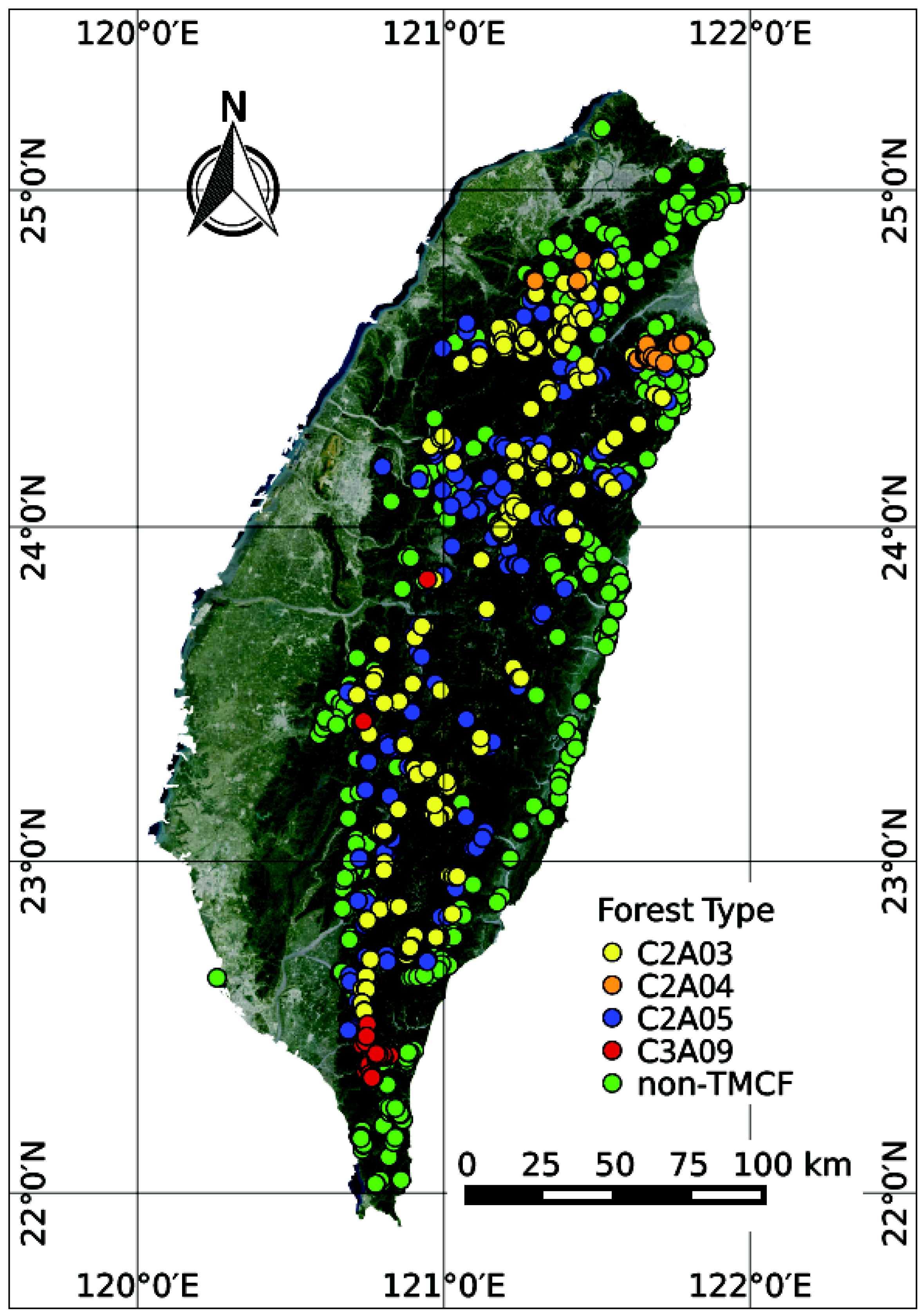
2.2.2. Vegetation Dataset

| Code | Forest Type | No. of plots |
|---|---|---|
| Tropical Montane Cloud Forest | ||
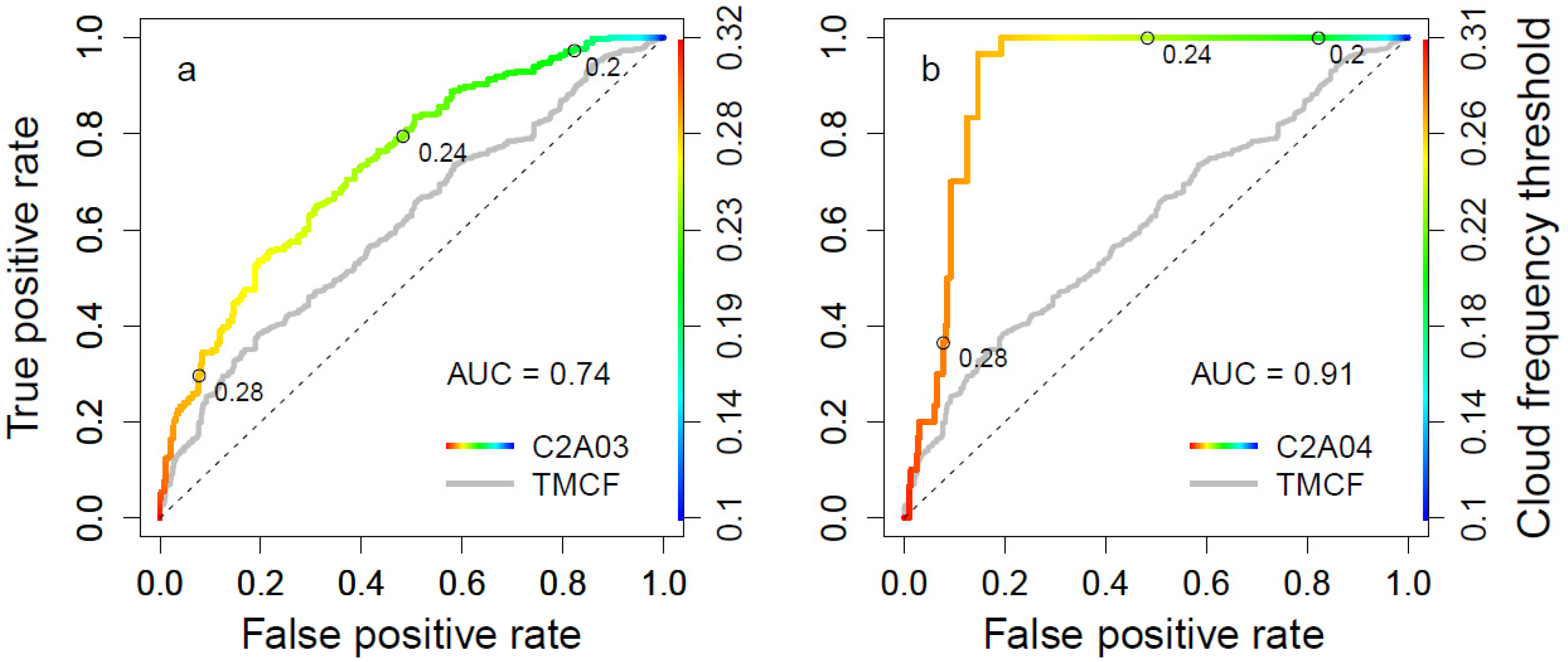
| C2A03 | Chamaecyparis montane mixed cloud forest | 383 |
| C2A04 | Fagus montane deciduous broad-leaved cloud forest | 30 |
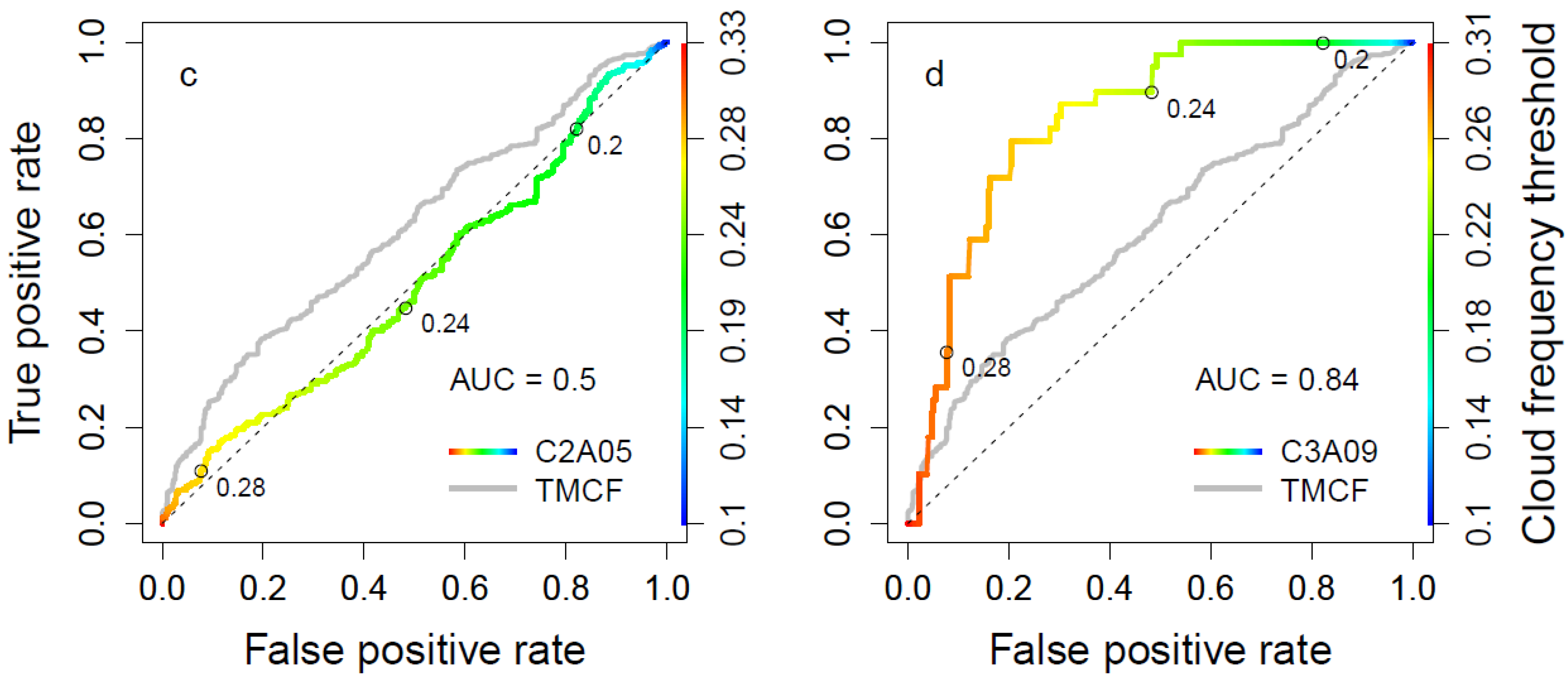
| C2A05 | Quercus montane mixed cloud forest | 565 |
| C3A09 | Pasania–Elaeocarpus montane evergreen broad-leaved cloud forest | 39 |
| TMCF plots | 1017 | |
| Non-Tropical Montane Cloud Forest | ||
| C2A06 | Machilus–Castanopsis sub-montane evergreen broad-leaved forest | 199 |
| C2A07 | Phoebe–Machilus sub-montane evergreen broad-leaved forest | 191 |
| C2A08 | Ficus–Machilus foothill evergreen broad-leaved forest | 56 |
| C3A10 | Drypetes–Helicia sub-montane evergreen broad-leaved forest | 134 |
| C3A11 | Dysoxylum–Machilus foothill evergreen broad-leaved forest | 6 |
| Non-TMCF plots | 586 | |
| All considered plots | 1603 | |

2.3. Methods
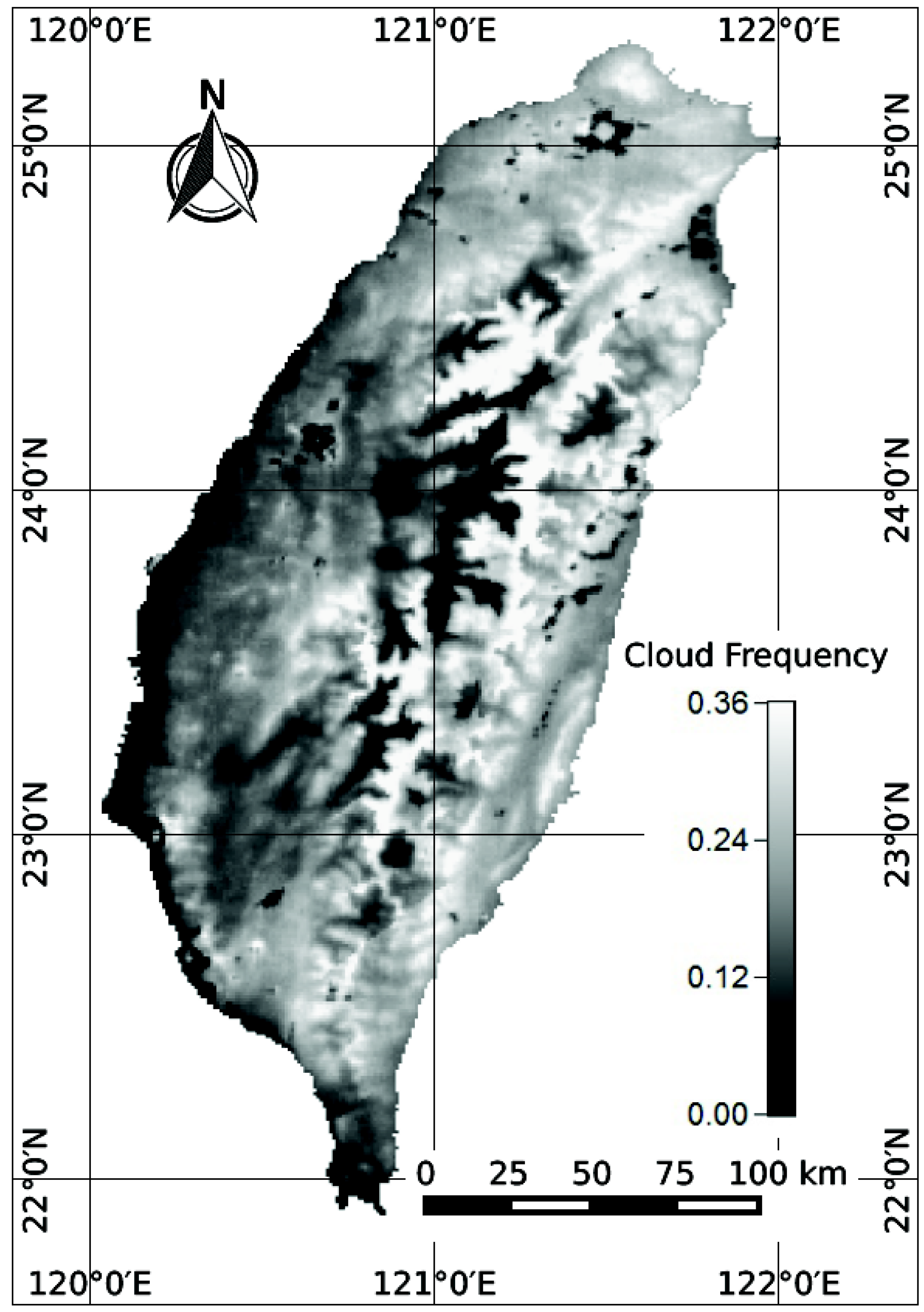
2.3.1. Calculation of the Low Cloud Frequency Map
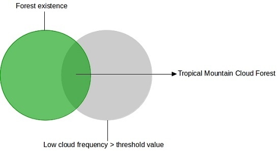
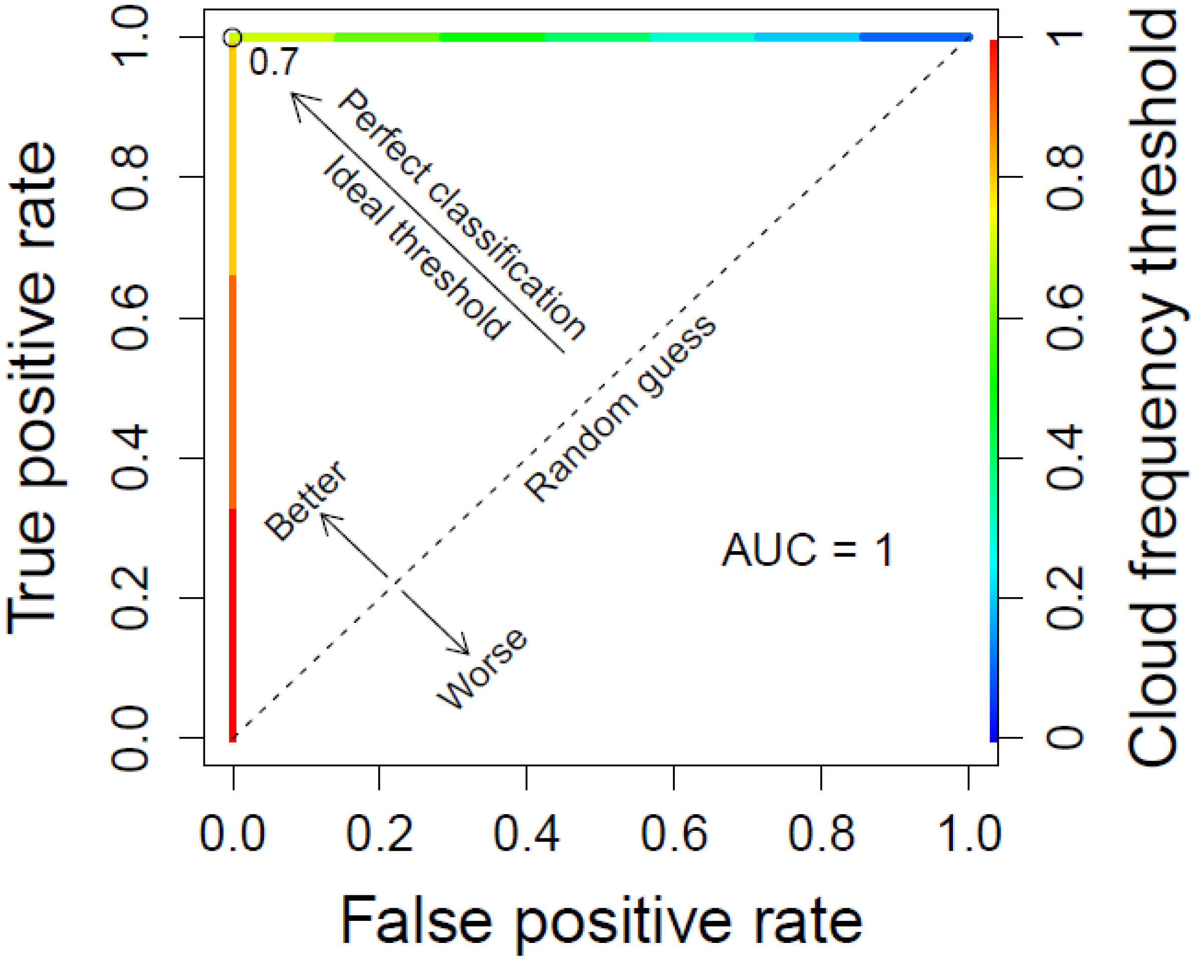
2.3.2. Investigating the Relationship between Cloud Forest Occurrence and Low Cloud Frequency
| Cloud Frequency | 1 | 0.9 | 0.8 | 0.7 | 0.6 | 0.5 | 0.4 | 0.3 | 0.2 | 0.1 | 0 |
|---|---|---|---|---|---|---|---|---|---|---|---|
| TMCF | 1 | 1 | 1 | 1 | 0 | 0 | 0 | 0 | 0 | 0 | 0 |
| Non-TMCF | 0 | 0 | 0 | 0 | 1 | 1 | 1 | 1 | 1 | 1 | 1 |

3. Results
3.1. Distribution and Frequency of Low Clouds
3.2. Relationship between Cloud Forest Occurrence and Low Cloud Frequency

4. Discussion
5. Conclusions
Acknowledgments
Author Contributions
Conflicts of Interest
References and Notes
- Hamilton, L.S. Mountain cloud forest conservation and research: A synopsis. Mount. Res. Dev. 1995, 15, 259–266. [Google Scholar] [CrossRef]
- Bruijnzeel, L.A.; Hamilton, L.S. Decision Time for Cloud Forest; IHP Humid Tropics Programme Series No. 13; IHP, UNESCO: Paris, France, 2000. [Google Scholar]
- Bubb, P.; May, I.; Miles, L.; Sayer, J. Cloud Forest Agenda; UNEP World Conservation Monitoring Centre: Cambridge, UK, 2004. [Google Scholar]
- Postel, S.L.; Thompson, B.H., Jr. Watershed protection: Capturing the benefits of nature’s water supply services. Natural Resources Forum 2005, 29, 98–108. [Google Scholar] [CrossRef]
- Hsieh, C.F. Composition, endemism and phytogeographical affinities of the Taiwan flora. Flora Taiwan 2003, 6, 1–14. [Google Scholar]
- Foster, P. The potential negative impacts of global climate change on tropical montane cloud forests. Earth-Science Rev. 2001, 55, 73–106. [Google Scholar] [CrossRef]
- Nadkarni, N.M.; Solano, R. Potential effects of climate change on canopy communities in a tropical cloud forest: An experimental approach. Oecologia 2002, 131, 580–586. [Google Scholar] [CrossRef]
- Ray, D.K.; Nair, U.S.; Lawton, R.O.; Welch, R.M.; Pielke, R.A. Impact of land use on Costa Rican tropical montane cloud forests: Sensitivity of orographic cloud formation to deforestation in the plains. J. Geophys. Res.: Atmos. 2006, 111. [Google Scholar] [CrossRef]
- Martínez, M.L.; Pérez-Maqueo, O.; Vázquez, G.; Castillo-Campos, G.; García-Franco, J.; Mehltreter, K.; Landgrave, R. Effects of land use change on biodiversity and ecosystem services in tropical montane cloud forests of Mexico. Forest Ecol. Manage. 2009, 258, 1856–1863. [Google Scholar] [CrossRef]
- Scatena, F.N.; Bruijnzeel, L.A.; Bubb, P.; Das, S. Setting the stage. In Tropical Montane Cloud Forests: Science for Conservation and Management; Bruijnzeel, L.A., Scatena, F.N., Hamilton, L.S., Eds.; Cambridge University Press: Cambridge, UK, 2010; pp. 3–13. [Google Scholar]
- Jarvis, A.; Mulligan, M. The climate of cloud forests. Hydrol. Process. 2011, 25, 327–343. [Google Scholar] [CrossRef]
- Frahm, J.P.; Gradstein, S.R. An altitudinal zonation of tropical rain forests using byrophytes. J. Biogeogr. 1991, 18, 669–678. [Google Scholar] [CrossRef]
- Campanella, R. The role of GIS in evaluating contour-based limits of cloud forest reserves in Honduras. In Tropical Montane Cloud Forests; Hamilton, L.S., Juvik, J.O., Scatena, F.N., Eds.; Springer: New York, NY, USA, 1995; pp. 116–124. [Google Scholar]
- Li, C.F.; Chytrý, M.; Zelený, D.; Chen, M.Y.; Chen, T.Y.; Chiou, C.R.; Hsia, Y.-J.; Liu, H.-Y.; Yang, S.-Z.; Yeh, C.-L.; et al. Classification of Taiwan forest vegetation. Appl. Veg. Sci. 2013, 16, 698–719. [Google Scholar] [CrossRef]
- Scholl, M.; Eugster, W.; Burkard, R. Understanding the role of fog in forest hydrology: stable isotopes as tools for determining input and partitioning of cloud water in montane forests. Hydrol. Process. 2011, 25, 353–366. [Google Scholar] [CrossRef]
- Bruijnzeel, L.A.; Mulligan, M.; Scatena, F.N. Hydrometeorology of tropical montane cloud forests: emerging patterns. Hydrol. Process. 2011, 25, 465–498. [Google Scholar] [CrossRef]
- Grubb, P.J.; Lloyd, J.R.; Pennington, T.D.; Whitmore, T.C. A comparison of montane and lowland rain forest in Ecuador I. The forest structure, physiognomy, and floristics. J. Ecol. 1963, 51, 567–601. [Google Scholar] [CrossRef]
- Stadtmüller, T. Cloud Forests in the Humid Tropics: A Bibliographic Review; United Nations University Press: Tokyo, Japan, 1987. [Google Scholar]
- Mulligan, M.; Burke, S.M. DFID FRP Project ZF0216 Global Cloud Forests and Environmental Change in a Hydrological Context; Final Report; DFID: London, UK, 2005. [Google Scholar]
- Elias, V.; Tesar, M.; Buchtele, J. Occult precipitation: sampling, chemical analysis and process modelling in the Sumava Mts., (Czech Republic) and in the Taunus Mts. (Germany). J. Hydrol. 1995, 166, 409–420. [Google Scholar] [CrossRef]
- Dawson, T.E. Fog in the California redwood forest: Ecosystem inputs and use by plants. Oecologia 1998, 117, 476–485. [Google Scholar] [CrossRef]
- Weathers, K.C.; Lovett, G.M.; Likens, G.E.; Caraco, N.F. Cloudwater inputs of nitrogen to forest ecosystems in southern Chile: Forms, fluxes, and sources. Ecosystems 2000, 3, 590–595. [Google Scholar] [CrossRef]
- Mildenberger, K.; Beiderwieden, E.; Hsia, Y. J.; Klemm, O. CO2 and water vapor fluxes above a subtropical mountain cloud forest—The effect of light conditions and fog. Agr. Forest Meteorol. 2009, 149, 1730–1736. [Google Scholar] [CrossRef]
- Mulligan, M. Modeling the tropics-wide extent and distribution of cloud forest and cloud forest loss, with implications for conservation priority. In Tropical Montane Cloud Forests: Science for Conservation and Management; Bruijnzeel, L.A., Scatena, F.N., Hamilton, L.S., Eds.; Cambridge University Press: Cambridge, UK, 2010; pp. 14–38. [Google Scholar]
- Ackerman, S.A.; Strabala, K.I.; Menzel, W.P.; Frey, R.A.; Moeller, C.C.; Gumley, L.E. Discriminating clear sky from clouds with MODIS. J. Geophys. Res.: Atmos. 1998, 103, 32141–32157. [Google Scholar] [CrossRef]
- Ackerman, S.A.; Holz, R.E.; Frey, R.; Eloranta, E.W.; Maddux, B.C.; McGill, M. Cloud detection with MODIS. Part II: validation. J. Atmos. Ocean. Tech. 2008, 25, 1073–1086. [Google Scholar]
- Ackerman, S.; Strabala, K.; Menzel, P.; Frey, R.; Moeller, C.; Gumley, L. Discriminating Clear-Sky from Cloud with MODIS Algorithm Theoretical Basis Document (MOD35); MODIS Cloud Mask Team, Cooperative Institute for Meteorological Satellite Studies, University of Wisconsin: Madison, WI, USA, 2010. [Google Scholar]
- Frey, R.A.; Ackerman, S.A.; Liu, Y.; Strabala, K.I.; Zhang, H.; Key, J.R.; Wang, X. Cloud detection with MODIS. Part I: Improvements in the MODIS cloud mask for collection 5. J. Atmos. Ocean. Tech. 2008, 25, 1057–1072. [Google Scholar] [CrossRef]
- Nair, U.S.; Asefi, S.; Welch, R.M.; Ray, D.K.; Lawton, R.O.; Manoharan, V.S.; Mulligan, M.; Sever, T.L.; Irwin, D.; Pounds, J.A. Biogeography of tropical montane cloud forests. Part II: Mapping of orographic cloud immersion. J. Appl. Meteorol. Climatol. 2008, 47, 2183–2197. [Google Scholar] [CrossRef]
- Cermak, J.; Bendix, J. Detecting ground fog from space—A microphysics-based approach. Int. J. Remote Sens. 2011, 32, 3345–3371. [Google Scholar] [CrossRef]
- Egli, S.; Maier, F.; Bendix, J.; Thies, B. Vertical distribution of microphysical properties in radiation fogs—A case study. Atmos. Res. 2015, 151, 130–145. [Google Scholar] [CrossRef]
- Chiou, C.R.; Hsieh, C.F.; Wang, J.C.; Chen, M.Y.; Liu, H.Y.; Yeh, C.L.; Yang, S.-Z.; Chen, T.-Y.; Hsia, Y.-J.; Song, G.Z.M. The first national vegetation inventory in Taiwan. Taiwan J. For. Sci. 2009, 24, 295–302. [Google Scholar]
- Yu, L.F.; Chen, Z.E.; Guo, T.H. Establishment of proper land-use assessment and management strategy for Deji Reservoir Catchment, Taiwan. Water Air, Soil Pollution: Focus 2009, 9, 323–338. [Google Scholar] [CrossRef]
- Klose, C. Climate and geomorphology in the uppermost geomorphic belts of the Central Mountain Range, Taiwan. Quatern Int. 2006, 147, 89–102. [Google Scholar] [CrossRef]
- Chen, C.S.; Chen, Y.L. The rainfall characteristics of Taiwan. Mon. Weather Rev. 2003, 131, 1323–1341. [Google Scholar] [CrossRef]
- Kao, S.C.; Kume, T.; Komatsu, H.; Liang, W.L. Spatial and temporal variations in rainfall characteristics in mountainous and lowland areas in Taiwan. Hydrol Process 2013, 27, 2651–2658. [Google Scholar] [CrossRef]
- Kerns, J.B.W.; Chen, Y.L.; Chang, M.Y. The diurnal cycle of winds, rain, and clouds over Taiwan during the Mei-Yu, summer, and autumn rainfall regimes. Mon. Weather Rev. 2010, 138, 497–516. [Google Scholar] [CrossRef]
- Taiwan Forestry Bureau. Available online: www.forest.gov.tw (accessed on 20 October 2014).
- Lin, C.W.; Tseng, C.M.; Tseng, Y.H.; Fei, L.Y.; Hsieh, Y.C.; Tarolli, P. Recognition of large scale deep-seated landslides in forest areas of Taiwan using high resolution topography. J. Asian Earth Sci. 2013, 62, 389–400. [Google Scholar] [CrossRef]
- Lee, M.F.; Lin, T.C.; Vadeboncoeur, M.A.; Hwong, J.L. Remote sensing assessment of forest damage in relation to the 1996 strong typhoon Herb at Lienhuachi Experimental Forest, Taiwan. Forest Ecol. Manag. 2008, 255, 3297–3306. [Google Scholar] [CrossRef]
- Mabry, C.M.; Hamburg, S.P.; Lin, T.C.; Horng, F.W.; King, H.B.; Hsia, Y.J. Typhoon disturbance and stand-level damage patterns at a subtropical forest in Taiwan. Biotropica 1998, 30, 238–250. [Google Scholar] [CrossRef]
- Suzuki, T. Forest Vegetation of East Asia; Kokin-Shoin: Tokyo, Japan, 1952. (In Japanese) [Google Scholar]
- Kira, T. A New Classification of Climate in Eastern Asia as the Basis for Agricultural Geography; Horticultural Institute Kyoto University: Kyoto, Japan, 1945. [Google Scholar]
- Hijmans, R.J.; Cameron, S.E.; Parra, J.L.; Jones, P.G.; Jarvis, A. Very high resolution interpolated climate surfaces for global land areas. Int. J. Climatol. 2005, 25, 1965–1978. [Google Scholar] [CrossRef]
- Fawcett, T. An introduction to ROC analysis. Pattern Recogn. Lett. 2006, 27, 861–874. [Google Scholar] [CrossRef]
- Sing, T.; Sander, O.; Beerenwinkel, N.; Lengauer, T. ROCR: Visualizing classifier performance in R. Bioinformatics 2005, 21, 3940–3941. [Google Scholar] [CrossRef] [PubMed]
- Chen, C.S.; Huang, J.M. A numerical study of precipitation characteristics over Taiwan Island during the winter season. Meteorol. Atmos. Phys. 1999, 70, 167–183. [Google Scholar] [CrossRef]
- Chen, T.C.; Yen, M.C.; Huang, W.R.; Gallus, W.A., Jr. An East Asian cold surge: Case study. Mon. Weather Rev. 2002, 130, 2271–2290. [Google Scholar] [CrossRef]
- Liou, Y.A.; Kar, S.K. Study of cloud-to-ground lightning and precipitation and their seasonal and geographical characteristics over Taiwan. Atmos. Res. 2010, 95, 115–122. [Google Scholar] [CrossRef]
- Shieh, S.L.; Wang, S.T.; Cheng, M.D.; Yeh, T.C. Tropical Cyclone Tracks over Taiwan from 1897 to 1996 and Their Applications; Central Weather Bureau Tech. Rep. CWB86-1M-01; Central Weather Bureau: Taipei, Taiwan, 1998. [Google Scholar]
- Tao, W.K.; Chen, C.S.; Jia, Y.; Lang, S. Two heavy precipitation events in Taiwan: Regional scale model simulations. In Proceedings of Workshop on Numerical Simulations of Precipitation in Taiwan Area, Chung-Li, Taiwan, 17–18 February 2000; pp. 19–20.
- Boyle, J.S.; Chen, T.J. Synoptic aspects of the wintertime East Asian monsoon. In Monsoon Meteorology; Chang, C.P., Krishnamurti, T.N., Eds.; Oxford University Press: Oxford, UK, 1987; pp. 125–160. [Google Scholar]
- Yeh, H.C.; Chen, Y.L. Characteristics of rainfall distributions over Taiwan during the Taiwan Area Mesoscale Experiment (TAMEX). J. Appl. Meteorol. 1998, 37, 1457–1469. [Google Scholar] [CrossRef]
- Chen, Y.L. Effects of island induced airflow on rainfall distributions during the Mei-Yu season over Taiwan. In Proceedings of Workshop on Numerical Simulations of Precipitation in Taiwan Area, Chung-Li, Taiwan, 17–18 February 2000; pp. 5–11.
- Aldrich, M.; Billington, C.; Edwards, M.; Laidlaw, R. A Global Directory of Tropical Montane Cloud Forests; UNEP–WCMC: Cambridge, UK, 1997. [Google Scholar]
- Lai, Y.J.; Chou, M.D.; Lin, P.H. Parameterization of topographic effect on surface solar radiation. J. Geophys. Res.: Atmos. 2010, 115. [Google Scholar] [CrossRef]
- Lai, Y.J.; Li, C.F.; Lin, P.H.; Wey, T.H.; Chang, C.S. Comparison of MODIS land surface temperature and ground-based observed air temperature in complex topography. Int. J. Remote Sens. 2012, 33, 7685–7702. [Google Scholar] [CrossRef]
- Schulz, H.M.; Thies, B.; Cermak, J.; Bendix, J. 1 km fog and low stratus detection using pan-sharpened MSG SEVIRI data. Atmos. Meas. Tech. 2012, 5, 2469–2480. [Google Scholar] [CrossRef]
© 2015 by the authors; licensee MDPI, Basel, Switzerland. This article is an open access article distributed under the terms and conditions of the Creative Commons Attribution license (http://creativecommons.org/licenses/by/4.0/).
Share and Cite
Thies, B.; Groos, A.; Schulz, M.; Li, C.-F.; Chang, S.-C.; Bendix, J. Frequency of Low Clouds in Taiwan Retrieved from MODIS Data and Its Relation to Cloud Forest Occurrence. Remote Sens. 2015, 7, 12986-13004. https://doi.org/10.3390/rs71012986
Thies B, Groos A, Schulz M, Li C-F, Chang S-C, Bendix J. Frequency of Low Clouds in Taiwan Retrieved from MODIS Data and Its Relation to Cloud Forest Occurrence. Remote Sensing. 2015; 7(10):12986-13004. https://doi.org/10.3390/rs71012986
Chicago/Turabian StyleThies, Boris, Alexander Groos, Martin Schulz, Ching-Feng Li, Shih-Chieh Chang, and Jörg Bendix. 2015. "Frequency of Low Clouds in Taiwan Retrieved from MODIS Data and Its Relation to Cloud Forest Occurrence" Remote Sensing 7, no. 10: 12986-13004. https://doi.org/10.3390/rs71012986
APA StyleThies, B., Groos, A., Schulz, M., Li, C.-F., Chang, S.-C., & Bendix, J. (2015). Frequency of Low Clouds in Taiwan Retrieved from MODIS Data and Its Relation to Cloud Forest Occurrence. Remote Sensing, 7(10), 12986-13004. https://doi.org/10.3390/rs71012986