Water Quality and River Plume Monitoring in the Great Barrier Reef: An Overview of Methods Based on Ocean Colour Satellite Data

Abstract

A strong driver of water quality change in the Great Barrier Reef (GBR) is the pulsed or intermittent nature of terrestrial inputs into the GBR lagoon, including delivery of increased loads of sediments, nutrients, and toxicants via flood river plumes (hereafter river plumes) during the wet season. Cumulative pressures from extreme weather with a high frequency of large scale flooding in recent years has been linked to the large scale reported decline in the health of inshore seagrass systems and coral reefs in the central areas of the GBR, with concerns for the recovery potential of these impacted ecosystems. Management authorities currently rely on remotely-sensed (RS) and in situ data for water quality monitoring to guide their assessment of water quality conditions in the GBR. The use of remotely-sensed satellite products provides a quantitative and accessible tool for scientists and managers. These products, coupled with in situ data, and more recently modelled data, are valuable for quantifying the influence of river plumes on seagrass and coral reef habitat in the GBR. This article reviews recent remote sensing techniques developed to monitor river plumes and water quality in the GBR. We also discuss emerging research that integrates hydrodynamic models with remote sensing and in situ data, enabling us to explore impacts of different catchment management strategies on GBR water quality.

1. Introduction

Coastal zones are experiencing increasing pressure from anthropogenic activities, compounded by a rapidly rising human population, with more than 60% of the world’s population located within the coastal zone [1,2]. Connections between environmental variability and ecological response can occur across a large range of interacting spatial, temporal, and organizational scales [3,4], which can influence, to various degrees, change in the natural system. Many approaches of management and policy have been applied to reduce these pressures in coastal zones globally [5], however, this is complicated by the highly dynamic characteristics of coastal zones, which can encompass a broad range of ecosystems and processes.

In dynamic coastal areas with complex marine ecosystems, such as the GBR (Great Barrier Reef) lagoon, it has been a challenge for managers to acquire evidence of ecological responses to biophysical drivers, such as declining water quality. The natural environmental variability, the diversity of ecosystems, and replication of data over sufficient spatial and temporal scales to provide an adequate baseline, confound this challenge [6]. Collecting information that reflects both natural and human-induced environmental changes at relevant scales is essential for decision making [6] and relevant to the successful monitoring of large geographical systems such as the GBR [7]. The GBR is also characterised by large regional, seasonal, and inter-annual variability, highlighting the need for capacity to measure water quality conditions at a range of temporal and spatial scales. RS technologies can provide the synoptic window necessary for the characterisation of marine ecosystems through enhanced spatial and temporal data resolution obtained from remote sensors [8,9].

Declining water quality from land-based runoff is one of the most significant threats to the health of the GBR, with sediments, nutrients, and pesticides identified as the key contaminants of concern [10]. Wet season conditions are experienced from December–April in Northern Australia and are an important catalyst in the condition and variability associated with water quality within the GBR [9]. On average, 70 km³ of freshwater is discharged each year by rivers and streams into the GBR lagoon [11]. River flow is delivered in discrete flood events during the five-month summer wet season, forming distinctive river plumes in the coastal zone that can move north along the coast but can occasionally move out towards the mid and outer reef area. The content of the river discharge has changed through time with large increases in the loads of sediments, nutrients, and pesticides associated with the expansion of agricultural development of the GBR catchment [10,11,12]. Persistent, above average river flows over a seven year period have been associated with a number of changes in the GBR communities, such as reduction in seagrass cover [13], impacts on coral cover, increase in coral disease [14], and high mortality rates of dugongs and turtles [15,16,17].

Management agencies in Australia are responding to these issues with the Australian and Queensland (State) Governments committing to the Reef Water Quality Protection Plan [10], a bilateral policy (initiated in 2003), that aims to ensure that ‘by 2020 the quality of water entering the GBR from broadscale land use has no detrimental impact on the health and resilience of the GBR’. The plan identifies a range of strategies and actions to achieve this goal including prioritisation of investment, adoption of improved land management practices, and evaluation of performance [18]. The Paddock to Reef Integrated Monitoring Program (P2R Program) [18] has been designed to support this evaluation and includes indicators of the adoption of improved land management practices, catchment condition, end of catchment pollutant load estimates, and marine water quality and ecosystem health. The marine component, known as the Marine Monitoring Program (herein referred to as the MMP), includes ambient and wet season water quality measurements, and inshore coral and seagrass health monitoring [13,19,20,21,22].

The onset and duration of river plumes into the GBR has been reported over several decades [20,23,24,25,26,27,28,29,30] and monitoring of river plumes [31] now forms an integral component of the MMP. However, it has been difficult to evaluate the complex responses of the seagrass and coral communities to changing water quality based on in situ water quality data only due to the limitations of the monitoring time frames and the uncertainty associated with the time lag between exposure and impact.

The use of RS (remotely-sensed) data in combination with in situ water quality measurements has provided a powerful source of data in the evaluation of water quality across the GBR. For example, river plumes have been mapped through a combination of aerial and satellite imagery and the coverage of GBR ecosystems visually assessed using satellite imagery [30,31,32]. More recently, RS studies using quasi-true colour (hereafter true colour) satellite images (Figure 1) and derived water quality level-2 products have been utilised to map and characterise the spatial and temporal distribution of GBR river plumes [28,33,34,35,36,37]. Recent work has also focused on the area and impact of these river plumes on GBR ecosystems [9,22,28,32,33,34,35,36,37,38,39].

To detect, map, and characterise these river plumes, remote sensors can exploit their differences in colour from ambient marine waters [40] (Figure 1). The optical signature of a river plume is related to the optical active constituents (hereafter OACs) of the water, including the presence and combination of chlorophyll-a, coloured dissolved organic matter (hereafter CDOM), and total suspended solids (hereafter TSS). Surface radiances are converted to reflectances, providing the spectral signatures required for quantifying the chlorophyll-a pigments, the CDOM, and the mineral suspended matter [40,41,42,43,44]. Monitoring OACs concentrations with RS techniques is notoriously challenging in optically complex (Case 2) coastal waters [8,45], which include the area of inshore GBR lagoon, typically within 20 km of the coast [35,37]. These limitations of the RS data must be understood and reported in order to efficiently use this data as an appropriate monitoring tool for the measurement and reporting of water quality in the GBR.

This paper reports on the application of RS data and imagery (MODIS (Moderate Resolution Imaging Spectroradiometer) radiances, reflectances, and Level-2 data) and the development of RS products that have been specifically adapted or designed for monitoring of water quality in the GBR. RS products presented here have been developed from post processing of RS data and applied in the monitoring of acute (river plumes) and chronic wet season water quality conditions in the GBR. We also acknowledge the current challenges in utilising these data sources, and describe future developments of integrating RS data and products with modelling outputs that will continue to extend our ability to make spatial and temporal assessments of water quality across the GBR.

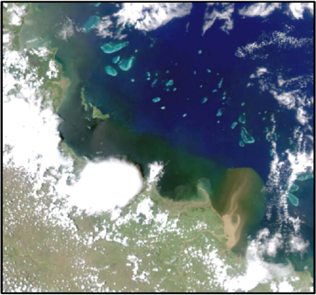
Figure 1. MODIS (Moderate Resolution Imaging Spectroradiometer) satellite true colour images (Level-1 data) showing river plume waters extending from the Burdekin River in the central GBR (Great Barrier Reef) and the influence of the river water on the colour of the surface waters.

Figure 1. MODIS (Moderate Resolution Imaging Spectroradiometer) satellite true colour images (Level-1 data) showing river plume waters extending from the Burdekin River in the central GBR (Great Barrier Reef) and the influence of the river water on the colour of the surface waters.

2. Data and Methods

2.1. Water Quality Monitoring in the GBR

The MMP was established in 2005 to monitor the GBR inshore environment through the assessment of long-term changes in the condition of inshore water quality, seagrass, and coral reefs. This inshore area is at highest risk from degraded water quality and makes up approximately 8 per cent of the GBR Marine Park and is generally within 20 km of the shore. The inshore area supports significant ecological communities and is also important for recreational visitors, commercial tourism operations, and commercial fisheries. The current water quality program includes: (1) in situ ambient and wet season monitoring of sediments, nutrients, and pesticides [31,46,47], and (2) through a range of remote sensing techniques supported by the development of regionally specific algorithms, producing regionally-tuned MODIS ocean colour products for the GBR [36,37].

2.2. In situ Water Quality Sampling

The ambient inshore MMP water quality program commenced in 2005, and targeted monitoring of wet season water quality data was initiated under the MMP in December 2007. This component of the MMP aims to investigate the acute and chronic influence of terrestrial runoff on inshore GBR water quality and coral and seagrass health [21,31,48]. This program samples the development and extent of the river plume waters, identifies concentration gradients of water quality parameters (i.e., salinity, temperature, particulate and dissolved nutrients, phytoplankton, suspended solids, Secchi depth, CDOM, chlorophyll-a, and pesticides) and characterises wet season water quality conditions in the GBR. Water sampling is initiated at the onset of the wet season, targeting the first flush, the rise, peak, and flux of the rivers entering the GBR lagoon. Depth profiling is conducted using Conductivity-Depth-Temperature (CTD) casts that measure vertical attenuation of light coefficients (Kd (PAR)), temperature, dissolved oxygen, and salinity. Generally, for the wet season monitoring, the water samples are collected in a series of transects away from the river mouth along the river-influenced areas within the GBR, including: the Normanby (14.4°S), Russell-Mulgrave and Tully (18°S), Herbert (18.5°S), Burdekin (19.5°S), Mackay WS, (20.7°S), and Fitzroy (23.5°S) regions (Figure 2). Water samples taken at the surface, and at depth, are usually taken over a period of days to weeks, dependent on the intensity of the event and the logistics of vessel deployment. The majority of samples are collected inside the visible extent of the river plume.

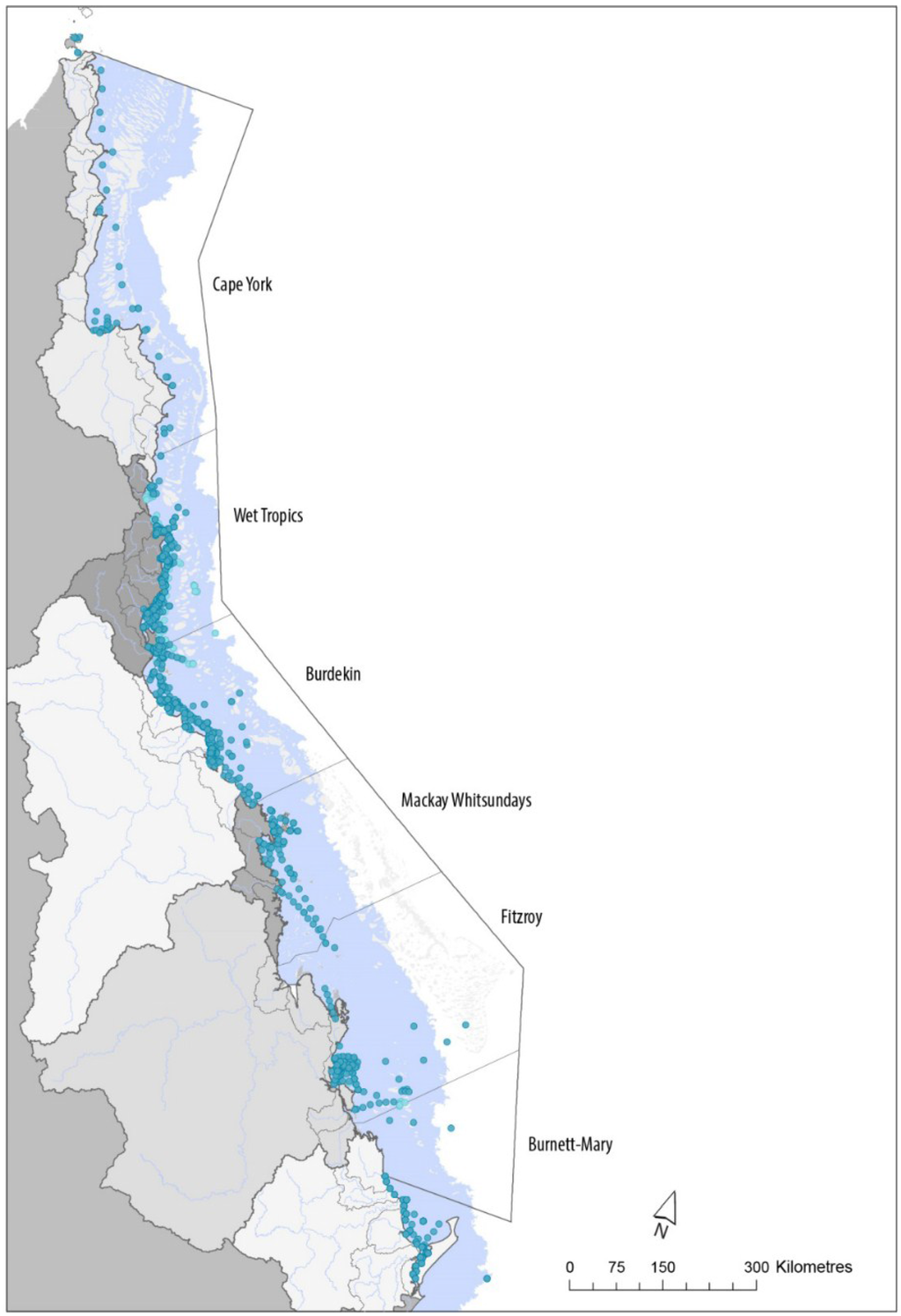
Figure 2. Selection of wet season sites sampled in the Northern, Central, and Southern GBR under the MMP (Marine Monitoring Program) (2006–2013). For full details, http://www.gbrmpa.gov.au/managing-the-reef/how-the-reefs-managed/reef-2050-marine-monitoring-program).

Figure 2. Selection of wet season sites sampled in the Northern, Central, and Southern GBR under the MMP (Marine Monitoring Program) (2006–2013). For full details, http://www.gbrmpa.gov.au/managing-the-reef/how-the-reefs-managed/reef-2050-marine-monitoring-program).

The monitoring of river plume and wet season conditions under the MMP over the last seven years has extended a comprehensive data set that has been used for characterising the temporal and spatial variability of coastal water quality in the GBR [30,31]. Work has built on assessments of a single GBR region, the Tully River in the Wet Tropics (Figure 2), over a 20-year time frame [32], to reporting wet season water quality over multiple catchments over multi-annual time frames [34,38]. Data collected under the MMP has also provided a key contribution to several research and monitoring projects [20,28,29,30,38,39,49,50,51,52], the continued validation required in the development of regionally based RS algorithms [36,37] and products [28,29,53,54] for the GBR, and for the validation of outputs generated by hydrodynamic models [53].

Regional differences and variability in water quality concentrations are evident between the six Natural Resource Management (NRM) Regions used for regional reporting (Figure 3). Concentrations of dissolved inorganic nitrogen (DIN) are highest in the waters associated with the Wet Tropics, Burdekin, and Fitzroy regions, with the highest TSS values in the Burdekin and Fitzroy regions. These variable concentrations represent the ecological risk to GBR ecosystems associated with different land activities [54].

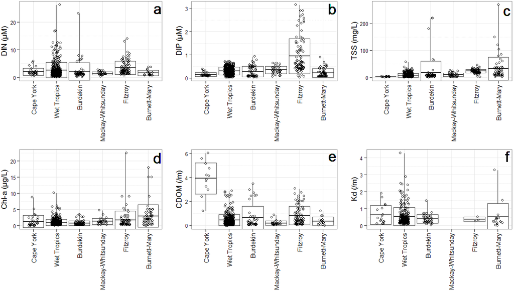
Figure 3. Boxplots displaying the water quality data collected within each of the Natural Resource Management (NRM) Regions in the GBR. Water quality plots are presented for (a) DIN, (b) Dissolved Inorganic Phosphorus, (c) TSS, (d) Chlorophyll-a, (e) CDOM (coloured dissolved organic matter) and (f) Kd (PAR). Data presented has been collected over an extended wet season period (Nov–May) from 2006 to 2014 under the MMP water quality Program. Boxplot presents the mean (dark black line), ±1 SD (rectangle), and maximum-minimum value (vertical lines). Nudge was applied to data on x-axis for better data visualisation.

Figure 3. Boxplots displaying the water quality data collected within each of the Natural Resource Management (NRM) Regions in the GBR. Water quality plots are presented for (a) DIN, (b) Dissolved Inorganic Phosphorus, (c) TSS, (d) Chlorophyll-a, (e) CDOM (coloured dissolved organic matter) and (f) Kd (PAR). Data presented has been collected over an extended wet season period (Nov–May) from 2006 to 2014 under the MMP water quality Program. Boxplot presents the mean (dark black line), ±1 SD (rectangle), and maximum-minimum value (vertical lines). Nudge was applied to data on x-axis for better data visualisation.

2.3. Remotely Sensed Satellite Data

2.3.1. Water Quality Products

Prior to RS imagery being easily accessible via free satellite imagery (from 2000), the dispersion of river plumes in the GBR lagoon was mapped using a combination of aerial photography, in situ water quality and salinity sampling from vessels [9,21,23]. Plumes are readily observable as brown turbid water masses contrasting with the clearer seawater, allowing the visible edge of the plume to be mapped at an altitude of 1000–2000 m in a light aircraft using a global positioning system (GPS). Plume dispersion was initially modelled based on salinity measurements [55]. These methods allowed a qualitative assessment of the extent of the river influence but are not able to retrieve estimates of water quality concentrations and information on the OACs.

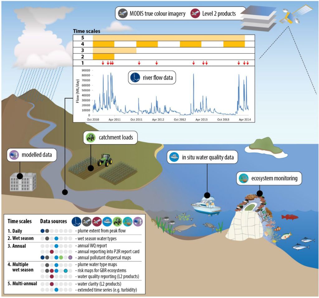
Figure 4. Conceptual model of the integration of data sources and the timing required to produce water quality monitoring products for the GBR. RS (remotely-sensed) products are described by the time scales available (daily, wet season, annual, multiple wet season, and multiple annual) and by the source of data that is required for the development of the product, including RS data (Level-1, Level-2), catchment load data, in situ data, modelled data, and ecosystem information (seagrass and coral reefs) for the GBR.

Figure 4. Conceptual model of the integration of data sources and the timing required to produce water quality monitoring products for the GBR. RS (remotely-sensed) products are described by the time scales available (daily, wet season, annual, multiple wet season, and multiple annual) and by the source of data that is required for the development of the product, including RS data (Level-1, Level-2), catchment load data, in situ data, modelled data, and ecosystem information (seagrass and coral reefs) for the GBR.

Satellite data provides a data source that can elucidate the composition of the surface water and provide a large source of data on coastal water quality processes. The extraction of satellite data involves complex and lengthy processing steps to go from the raw data stream (Level-0 data) through to maps of selected parameters and products (Level-3 data). The stages in this conversion process are known as product levels (or processing levels) and there is a canonical terminology used by remote sensing agencies and scientists and will be utilised in this manuscript to differentiate the different GBR products [56] (Table 1).

The use of true colour data, in combination with in situ wet season data and hydrodynamic models, has been instrumental in advancing many aspects of our understanding of water quality in the GBR. This has been achieved with a transition from a 1-dimensional tool that provided information on the visible extent of freshwater flow to 3-dimensional models that allow us to investigate the extent, duration, and content of river plume water types in the GBR and the level of exposure of GBR ecosystems. The processing associated with RS data and the RS products, combined with other sources of data, for wet season monitoring is illustrated in Figure 4.

The reporting of water quality through RS products for the GBR has been separated by the type of products described as either (i) annual monitoring Level-3 products derived from Level 2 data, (ii) wet season Level-3 products derived from Level 2 data, or (iii) wet season Level-3 products based on true colour. We will briefly describe all three categories of RS products and report in greater detail on the third category to outline the advances associated with the mapping of wet season and flood plume characteristics in the GBR. In addition, Table 2 [28,30,31,32,33,34,35,36,37,39,51,57,58,59,60,61,62,63,64,65,66,67,68,69,70] summarises the outputs associated with different approaches and products employed to map, report, and describe water quality in the GBR, and documents the advantages and disadvantages of each technique. The approaches that have been utilised in mapping of river plumes and wet season conditions are not always directly comparable, but are examples of the many different data sources that can provide information on events that are variable in space and time and can potentially impact across much longer time frames.

Table 1. Terminology associated with the different processing steps to create levels of remotely sensed data. Terminology derived from [56].

Level	Description	Example
0	Reconstructed, unprocessed instrument and payload data at full resolution, with any and all communications artefacts (e.g., synchronisation frames, communications headers, and duplicate data) removed.	Raw data—Ocean Colour
1a	Reconstructed, unprocessed instrument data at full resolution, time-referenced, and annotated with ancillary information, including radiometric and geometric calibration coefficients and georeferencing parameters.	True Colour
2	Derived geophysical variables (e.g., ocean wave height, temperature, TSS) at the same resolution and location as Level 1 source data.	TSS CDOM Chlorophyll-a
3	Variables mapped on uniform space/time grid scales, usually with some completeness and consistency (e.g., missing points interpolated, complete regions mosaicked together from multiple orbits, etc.)	Remapped (gridded) product based on geophysical values—multiannual time scales

Table 1. Terminology associated with the different processing steps to create levels of remotely sensed data. Terminology derived from [56].

Level	Description	Example
0	Reconstructed, unprocessed instrument and payload data at full resolution, with any and all communications artefacts (e.g., synchronisation frames, communications headers, and duplicate data) removed.	Raw data—Ocean Colour
1a	Reconstructed, unprocessed instrument data at full resolution, time-referenced, and annotated with ancillary information, including radiometric and geometric calibration coefficients and georeferencing parameters.	True Colour
2	Derived geophysical variables (e.g., ocean wave height, temperature, TSS) at the same resolution and location as Level 1 source data.	TSS CDOM Chlorophyll-a
3	Variables mapped on uniform space/time grid scales, usually with some completeness and consistency (e.g., missing points interpolated, complete regions mosaicked together from multiple orbits, etc.)	Remapped (gridded) product based on geophysical values—multiannual time scales

2.3.2. Annual Water Quality Products from Level-2 Data (Table 2; I, II)

RS techniques are a cost-effective method of determining spatial and temporal variation in near-surface concentrations of water quality parameters throughout the year. Retrieval and monitoring of annual water quality data in the GBR is achieved through the acquisition, processing using bio-optical algorithms, and validation of geo-corrected satellite ocean colour imagery, and i referred to hereafter as Level-2 products (Table 1). In the GBR, the key source of ocean colour data has been the Moderate Resolution Imaging Spectroradiometer [71] on board the NASA Earth Observing System (EOS) Aqua platform. This data has been primarily used because MODIS sensors have an adapted spatial resolution (250–1000 m resolution) and can provide up to 2 images per day of the GBR waters.

As part of the MMP water quality program, regional algorithms were developed to provide better satellite retrieval of water quality concentrations in the optically complex coastal waters, or case II waters, of the GBR than the “NASA global algorithms” implemented in the SeaWiFS Data Analysis System (SeaDAS [72]) (the NASA’s comprehensive image analysis package for the processing, display, analysis, and quality control of ocean colour data [36,37,57,58,60,72]). This work has provided regionally parameterised inversion algorithms, including (i) the artificial neural network atmospheric correction and (ii) the adaptive linear matrix (aLMI) inversion algorithm for deriving chlorophyll-a, TSS, and CDOM [58,72]. These algorithms are now routinely used to provide regionally-tuned ocean-colour products from MODIS-Aqua satellite imagery. This regional parameterised, remote sensed chlorophyll-a, TSS, and CDOM data can be acquired as daily, annual, or multi-annual products from the eReefs Marine Water Quality dashboard [73]. The satellite data is derived from cloud-free daytime imagery and processed using SeaDAS [72] and the Bureau Operational Ocean Colour (BOOC) data-processing package [73]. These GBR specific ocean colour products, particularly CDOM, have also contributed to additional methods of mapping the extent and composition of river plume waters [29] (see Section 2.3.3).

Recent work also includes the development of a regional bio-optical algorithm for determining regional Secchi depth (ZSD) related to turbidity, clarity, and TSS in coastal waters in GBR waters over wet and dry seasons [59,61]. This algorithm has been used to calibrate MODIS time series of photic depth in GBR waters using inshore water quality collected through long-term monitoring programs [74,75]). The correlations between river loads of fine sediment (or proxies for these loads) and remote-sensed photic depth have been reported across the GBR [61]. For years of high river flow and large fine sediment loads, strong correlations are found across the entire GBR shelf. The correlations are strongest inshore in water depths of less than 20 metres and weaker correlations are observed further offshore. The effect of lower clarity in large river discharge years is driven by the river plume-delivered fine material, which contains large amounts of organic material in flocs [76] being resuspended in periods of strong winds and large tides (a characteristic in the central-southern GBR). This work is an integral part of recent work on modelling the influence of river flow and suspended sediments on the dry season turbidity of the GBR [59,61].

However retrieval of RS water quality data in Case II waters is complex. It requires ongoing annual validation, particularly in response to sensor drift, including the evaluation of the regional algorithms performance associated with water types in different GBR regions and through the different seasons to ensure confidence in monitoring and assessment of water quality in the GBR [57,60,77].

2.3.3. Wet Season Water Quality Products from Level-2 Data (Table 2; III, IV, V)

Gradients of water quality within river plumes are highly dynamic, with deposition of the fine suspended sediment concentrations occurring close to the coast in lower salinity waters [38,76,78] and rapid transformations between nutrients, turbidity, and phytoplankton. These processes are difficult to fully capture with a traditional water quality program and RS data can provide a valuable dataset to fully capture these processes over adequate spatial and temporal scales.

The regionally parameterised Level-2 water quality product, CDOM, (m⁻¹) has been used to define the river plume extent through the relationship between CDOM and salinity, with a threshold CDOM value of 0.24 m⁻¹ corresponding to a salinity value of 30 (±4) ppt representing the outer edge of the river plumes [27]. This relationship between CDOM and salinity has also been the basis of a preliminary assessment between CDOM, as the proxy for freshwater extent, and exposure to Photosystem II-inhibiting herbicides (hereafter PSII herbicides) [51,62]. This work found a significant positive association between CDOM and exposure to PSII herbicides in the Wet Tropics; however, there is an increased occurrence of the uncertainties around satellite retrieval during the wet season, when PSII herbicide exposures are typically higher, potentially confounding the results. MODIS Level-2 satellite data has also been used to characterise external boundaries of river plumes and water types within GBR river plumes using supervised classification of MODIS Level 2 satellite data processed by the NASA standard algorithms and a combination of CDOM, chlorophyll-a, and TSS (estimated from two RS proxies) threshold values [34].

Quantifying uncertainties inherent to the water quality monitoring datasets (satellite or in situ) is crucial in determining how accurate the designed water quality products are, and in identifying the best data sets and information sources for specific regions or seasons of the GBR. This is particularly relevant for the retrieval of Level-2 RS data in the complex coastal Case II waters of the GBR. Improvements in deriving data from Case II waters is ongoing, both at a GBR and an international scale, and requires extensive validation across coastal water types, particularly in wet season conditions where high concentrations of suspended sediment and CDOM co-occur with phytoplankton in river plume waters. To define and map wet season conditions, particularly through periods of high river flow, “alternative” RS methods based on the extraction and analysis of MODIS true colour data have been tested and are described more fully in the following section.

2.3.4. Wet Season WQ Products from True Colour (Level-1 Data) (Table 2; VI–XI)

In the GBR region, the use of MODIS true colour imagery has provided a spatially rich technique in the estimation of river plume extent and improved the assessment of the level of exposure of inshore coral reefs and seagrass meadows to river plumes. River plume mapping utilising true colour imagery has been applied as a method of characterising the water quality conditions associated with periods of elevated river flow. Various products have been produced using different methods of extraction, aggregation through annual and multi-annual time frames, and integration to provide robust information on wet season conditions and to report decadal time frames (2002–2015) of water quality status.

(a) Mapping Extent of River Plumes (Table 2; VI)

River plumes maps are produced using MODIS Level-0 data acquired from the NASA Ocean Colour website (http://oceancolor.gsfc.nasa.gov) and converted into true-colour images with a spatial resolution of 500 m × 500 m using SeaDAS [72]. The true colour images are then spectrally enhanced from Red-Green-Blue to Hue-Saturation-Intensity colour systems and classified to six distinct river plumes water types defined by their colour (RGB/HSI signatures) properties (Figure 5, [63]) and hereafter referred to as plume colour classes. The clustering of the colour classes into six groups characterising the water types in the river plumes is through supervised classification using spectral signatures from the changes in colour associated with the gradient of river plumes. Each of the defined six colour classes (CC1–CC6) is characterised by different concentrations of optically active components (TSS, CDOM, and chlorophyll-a) which influence the light attenuation and can vary the impact on the underlying ecological systems. CC1–CC3 correspond to the brownish turbid water masses with high sediment and CDOM concentrations, CC4 and CC5 to the greener water masses with lower sediment concentrations favoring increased coastal productivity, and CC6 is the transitional water mass between plume waters and marine waters.

Figure 5. Triangular colour plot showing the characteristic colour signatures of the Great Barrier Reef river plume waters (six plume colour classes) in the Red-Green-Blue space. A method has been developed to map the GBR river plumes and the different water masses inside the river plumes using these characteristic signatures and a supervised classification of MODIS true colour data [63].

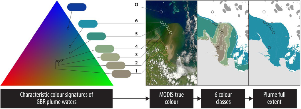
Figure 5. Triangular colour plot showing the characteristic colour signatures of the Great Barrier Reef river plume waters (six plume colour classes) in the Red-Green-Blue space. A method has been developed to map the GBR river plumes and the different water masses inside the river plumes using these characteristic signatures and a supervised classification of MODIS true colour data [63].

These river plume maps are processed into weekly and multi-week (wet season, multi-seasonal) composite maps [28,30,31,32,33,34,35]. This method is used to map the extent, movement, and frequency of occurrence of river plumes in the GBR during the wet season. The production of river plume maps has changed the perception that river plumes are nearly always constrained to the coast, with recognition that river plume waters with elevated concentrations of chlorophyll and CDOM can be mapped at large distances offshore and move hundreds of kilometers north, particularly those out of the larger dry tropics rivers (Figure 6a). However, despite the occasional offshore movement of the river flood plumes, the main areas of inundation and exposure are found with 25 km along the Queensland coast, with the strong prevailing south-easterlies driving a dominant northerly movement of river plumes along the GBR.

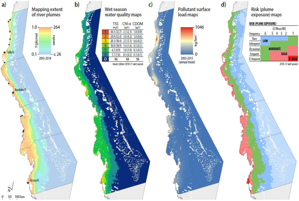
Figure 6. Outputs, expressed as GBR spatial maps, from the analysis and processing of true colour (Level-1) data extracted across the GBR. Maps include: (a) the extent and frequency of river plume in the GBR, reported as a multi-seasonal value for the period 2003–2013. The frequency value is calculated as the number of weeks within the wet season (December–April, ca. 22 weeks) over the 10-year period in which the pixel was exposed to river plume waters. River plume was identified by the extraction of colour class categories (CC1–CC6); (b) wet season water quality maps showing the mean colour class associated with each pixel for the wet season period December 2010–April 2011. Each colour class category is described by mean water quality values for TSS, CDOM, chlorophyll-a, and Kd (PAR); (c) surface load maps (or concentration maps) of Dissolved Inorganic Nitrogen (DIN) representing the mean surface concentration of DIN (reported as µM) per 500 m × 500 m pixel for the wet season period December 2010–April 2011; and (d) spatial risk maps showing the qualitative categories of risk associated with different permutations of plume frequency (as a proxy for intensity of impact) and the mean colour class value (as a proxy for the water quality concentration gradient).

Figure 6. Outputs, expressed as GBR spatial maps, from the analysis and processing of true colour (Level-1) data extracted across the GBR. Maps include: (a) the extent and frequency of river plume in the GBR, reported as a multi-seasonal value for the period 2003–2013. The frequency value is calculated as the number of weeks within the wet season (December–April, ca. 22 weeks) over the 10-year period in which the pixel was exposed to river plume waters. River plume was identified by the extraction of colour class categories (CC1–CC6); (b) wet season water quality maps showing the mean colour class associated with each pixel for the wet season period December 2010–April 2011. Each colour class category is described by mean water quality values for TSS, CDOM, chlorophyll-a, and Kd (PAR); (c) surface load maps (or concentration maps) of Dissolved Inorganic Nitrogen (DIN) representing the mean surface concentration of DIN (reported as µM) per 500 m × 500 m pixel for the wet season period December 2010–April 2011; and (d) spatial risk maps showing the qualitative categories of risk associated with different permutations of plume frequency (as a proxy for intensity of impact) and the mean colour class value (as a proxy for the water quality concentration gradient).

(b) Wet Season Water Quality Maps (Table 2; VII)

Wet season water quality maps are defined as maps where water quality concentrations associated with the level of land-sourced contaminants are measured or predicted, and are produced by normalising the frequency of the plume colour classes over multi-year time scales (Figure 6b). Information on plume water quality can then be extracted from these frequency maps by reporting the characteristics of the corresponding in situ wet season water quality data with the colour class or plume water type frequency values. Several land-sourced pollutants are investigated through match-ups between in situ data and the six plume colour class maps. Dissolved inorganic nitrogen (DIN), dissolved inorganic phosphorus (DIP), TSS, chlorophyll-a, Kd (PAR), and CDOM have all shown consistent patterns of variation across the six-colour classes (Figure 7). All these parameters present a general reduction trend from CC1 (more inshore waters)–CC6 (more offshore waters). The wet season water quality maps are produced as multi-week (wet season, multi-season) composite maps for the GBR [30,33,34]. Composite, multi-seasonal plume colour class maps (Figure 6b) provide a more broad-scale approach to reporting contaminant concentrations in the GBR marine environment and to map the range of statistical values (average, minimum, maximum) from the long term multi-seasonal water quality values associated with the colour class values.

Figure 7. Box plot representing the data collected on two water quality measurements (a) Dissolved Inorganic Nitrogen, DIN (µM) and (b) Dissolved Inorganic Phosphorus, DIP (µM), the three main optical attenuating components of (c) TSS (mg/L), (d) CDOM (m⁻¹), (e) chlorophyll-a (µg/L), and (f) light attenuation (Kd)PAR), m⁻¹), are shown over each river plume colour class and “out of the plume” in wet season conditions. Boxplot presents the mean (dark black line), ±1 SD (rectangle) and maximum-minimum value (vertical lines). Nudge was applied to data on x-axis for better data visualization. Data is sourced from the Wet Season water quality monitoring program under the MMP between 2007 and 2015.

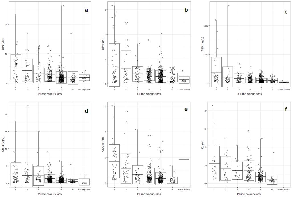
Figure 7. Box plot representing the data collected on two water quality measurements (a) Dissolved Inorganic Nitrogen, DIN (µM) and (b) Dissolved Inorganic Phosphorus, DIP (µM), the three main optical attenuating components of (c) TSS (mg/L), (d) CDOM (m⁻¹), (e) chlorophyll-a (µg/L), and (f) light attenuation (Kd)PAR), m⁻¹), are shown over each river plume colour class and “out of the plume” in wet season conditions. Boxplot presents the mean (dark black line), ±1 SD (rectangle) and maximum-minimum value (vertical lines). Nudge was applied to data on x-axis for better data visualization. Data is sourced from the Wet Season water quality monitoring program under the MMP between 2007 and 2015.

(c) Pollutant Surface Load Maps (Table 2; VIII, IX)

Pollutant surface load maps integrate three sources of data to map the dispersion of land-sourced pollutants. The load maps are produced by combining in situ data collected in the wet season (ca. December–April, inclusive) with river plume maps derived from MODIS true colour imagery (Figure 6c) and annual monitored end-of-catchment pollutant load [79]. River discharge in the wet season accounts for 78% of the total annual discharge (Department of Natural Resources and Mines, http://watermonitoring.dnrm.qld.gov.au/host.htm), so even though water quality parameters and river plume maps are for the wet season period only, they are used to produce annual load maps by incorporating annual pollutant loads delivered into the GBR for each river [80,81,82]. The in situ water quality data provides the pollutant mass variation as a function of the movement of the river plume away from the river mouth. The satellite imagery provides the direction and intensity of the pollutant mass dispersal over the GBR lagoon. As a result, this method produces an estimate of pollutant surface dispersion into the GBR, expressed in mass per area, generating a map of the “potential” risk of pollutant exposure in the marine environment for TSS, DIN, and particulate nitrogen (Figure 6c, [82]). The pollutant surface load maps within the GBR are produced as annual and multi-annual composite maps. As an example, the multi-annual map of DIN is shown for the period between 2003 and 2013, with the colour gradient representing the variation in the mean surface DIN reported as mass per area (kg/ha) (Figure 6c).

(d) GBR Plume Risk Maps (Table 2; X)

The river plume maps and wet season water quality maps can be overlaid with information on the presence or distribution of “contamination receptors”, i.e., GBR ecosystems susceptible to the land-sourced contaminants. This method can help identify ecosystems which may experience acute or chronic high exposure to contaminants in river plumes (exposure assessment) and, thus, help evaluate the susceptibility of GBR ecosystems to land-sourced contaminants [64]. For example, a recent study [39], mapped the occurrence of turbid water masses in Cleveland Bay (Burdekin marine region, Figure 1) in each wet season between 2007 and 2011 and compared the results to changes in the seagrass community. This analysis, realised though the production of plume frequency maps (Figure 6b), correlated with measurements of seagrass area and composition. The correlation indicated that the decline in seagrass meadow area and biomass was positively linked to high occurrence of turbid water masses and confirmed the impact that decreased clarity can have on seagrass health in the GBR [64,65,83].

One step further toward the production of “risk” maps for GBR ecosystems (Figure 6d) is to compare predicted pollutant concentration in river plumes (Figure 6b) to published ecological threshold values for ecological consequences [83,84] and combine this information to estimate the probability of environmental harm from exposure to river plumes and degraded water quality. Examples of these consequences include, but are not limited to, increased bleaching susceptibility in coral from nitrate exposure [85], phytoplankton blooms enhancing Crown of Thorn outbreaks from increased DIN loads [66,86,87], and reduced resilience in seagrass and corals due to reductions in light availability [83]. Ideally, the risk models should incorporate the potential of cumulative impacts [85,86] from multiple pollutants in river plume waters and the susceptibility of specific ecosystems (seagrass or coral reefs) should be taken into account [67,87]. This exercise is, however, challenging because the response of GBR ecosystems to an amount and/or duration of exposure to land-sourced contaminants (respectively or combined) in river plume waters is often unknown at a regional or ecosystem level [87]. Work in this area has progressed by using time series data of MODIS river plume water masses [33,68] to establish measures of frequency (as a proxy for intensity) (Figure 6a) with water quality gradients measured through the mapping of the 6CC’s. These maps can help summarise the likelihood and magnitude of the river plume risk, by spatially clustering water masses with different concentrations and proportions of land-sourced contaminants against a risk framework (Figure 6d). This framework produces river plume risk maps for seagrass and coral ecosystems based on a simplified risk matrix [33]. The “risk” of elevated nutrients and sediments needs to be closely linked to research identifying ecological thresholds to allow the qualitative framework expressed in Figure 6d to move to quantitative thresholds that can influence ecosystem decline and impact on GBR resilience [64,68,69,84]. Knowledge of these thresholds can identify ecosystems which may experience acute or chronic high exposure to contaminants in river plumes and help evaluate the susceptibility of GBR ecosystems to land-sourced contaminants. Spatial maps of potential risk associated with water quality thresholds are also an important data visualization tool for communicating environmental risks to managers and providing information on prioritising land based management. Work is in progress to test and improve this approach [68].

(e) Future Applications—Integration with Models (Table 2; XI)

Recent work has focused on the integration of empirically derived products with hydrodynamic models. Virtual (modelled) river tracers [53,70] allow the assessment of the relative pollutant contribution of each watershed to observed river plume characteristics and the impacts that different land management scenarios will have on river plume-ecosystem interactions. For example, this approach is being combined with coral trajectory models, to assess the future vulnerability of reefs to both local (water quality) and global (climate change) stressors [88]. Initial analysis has used in situ samples to calibrate river tracers to better reflect DIN spatial and temporal dynamics. Results will help with marine spatial planning decision making, by identifying those reefs that will most benefit from land management improvements, and which catchments should be prioritized from a cost-benefit point of view.

Table 2. Examples of remote sensed products currently applied in water quality monitoring of the Great Barrier Reef. Products in bold relate to analysis of true colour data collected in the wet season only. Based on MODIS data 2002–2014, processed into single-day and multi-day (week, month, season, and annual) composite maps. MODIS products also require continued access to in situ water quality monitoring data for parameterisation and validation. WQ = water quality.

Product Name	Description/Key Processes	Data Source	Advantages	Disadvantages	References
Annual monitoring–Level 3 products
I: Marine water quality indices for the GBR (Chla, NAP and CDOM)	MODIS time series of water quality indices in GBR waters (Level 2 products) using regionally paramaterised bio-optical algorithms: Artificial Neural Network (CROC-ANN) and Linear Matrix Inversion (aLMI).	MODIS imagery + CSIRO regional algorithm + The eReefs research platform (operational production at BOM a) In situ water quality data for validation	- High spatial and temporal coverage - No costs associated with the MODIS imagery - Account for atmospheric Correction - Valuable quantitative WQ information, such as the WQ concentration of CDOM, TSS, chlorophyll-a, or Z%	- Data from 2002 only. - High processing requirements - Retrieval of L2 data notoriously challenging in optically complex (Case 2) coastal waters ➔ need for regionally-tuned and validated algorithms	[36,37,57,58,60]
II: Marine water clarity for the GBR (Z%)	MODIS time series of photic depth in GBR waters using a regionally tuned bio-optical algorithm. This algorithm has been implemented to intensively describe the effects of river run-off on water clarity of the central GBR	MODIS imagery + University of Queensland algorithm Secchi depth (ZSD) data for validation			[59,61]
Wet season monitoring–Level 2 products
III: River plume maps (extent) for the GBR	MODIS time series of River plume extent based on a CDOM threshold correlated to 34ppt salinity. Level 2 CDOM value converted to salinity. Annual measurements of exceedance (1) or non exceedance (0)	Marine CDOM product for the GBR (product I)	- High spatial and temporal coverage - No costs associated with the MODIS imagery - Account for atmosphericCorrection - Valuable quantitative WQ information, such as the WQ concentration of CDOM	- Data from 2002 only. - Use regional Level 2 CDOM products: high uncertainty associated with Case 2 waters, particularly in plume conditions with high TSS, chlorophyll-a, and CDOM.	[28]
IV: Marine PSII (Photosystem II herbicides) maps for the GBR	MODIS time series of Photosystem II (PSII) herbicides in GBR waters. Based on correlation between the marine CDOM product for the GBR (product I: used as a proxy for salinity) and PSII herbicides concentrations. Focused on wet season data only.	Marine CDOM product for the GBR (product I) PS II herbicide concentration data	- High spatial and temporal coverage - No costs associated with the MODIS imager - Account for atmospheric Correction	- The threshold method assumes fixed WQ CDOM concentration thresholds to delineate and thus ignores potential temporal and spatial variability	[51,62]
V: River plume maps (extent and plume water types) for the GBR	MODIS time series of river plume extent and of three plume water types using supervised classification of MODIS Level 2 satellite data processed by the NASA standard algorithms and a combination of CDOM, Chlorophyll a and TSS (estimated from two RS proxies). Identification of potential L2/WQ threshold values.	MODIS imagery + NASA global algorithms + In situ WQ data from the flood plume program of the MMP	- High spatial and temporal coverage - No costs associated with the MODIS imagery - Account for atmosphericCorrection	- Data from 2002 only. - Use standard Level 2 CDOM, chlorophyll, and TSS proxy products: high uncertainty associated with Case 2 waters, particularly in plume conditions with high TSS, chlorophyll-a, and CDOM. - The L2 threshold method assume fixed WQ value/ concentration thresholds to delineate plumes and plume water types and thus also ignores potential temporal and spatial variability	[33,34]
Wet season monitoring–True colour products
VI: River plumes maps (extent and water types) for the GBR	MODIS time series of river plume extent and six plumes water types defined by their colour (RGB/HSI signatures) properties. Based on a supervised classification using spectral signatures from river plume water in the GBR.	MODIS true colour imagery	- High spatial and temporal coverage - No costs associated with the MODIS imagery - Simple and objectivemethod by clustering the information contained in MODIS true colour composites (Red Green Blue bands)	- Data from 2002 only. - High processing requirements - Relies on non-atmospherically corrected data - The spectral signature used to classify images does not incorporate potential temporal and spatial variability. - Quantitative WQ information (WQ concentrations) not directly available through the clustering of the true-colour composites.	[28,30,31,32,33,34,35,63]
VII: a) Wet season frequency maps of colour class and b) wet season water quality maps for the GBR	(a) MODIS time series of maps representing the multi-seasonal frequency of occurrence of the six colour classes. (b) MODIS time series of maps presenting potential concentrations (mean, min, max) of land-sourced pollutants linked to normalised frequency values of the six colour classes representing the water types across river plume	MODIS River plumes maps (extent and water types) for the GBR (Product VI) + In situ water quality data correlated with colour class frequency	- High spatial and temporal coverage No costs associated with the MODIS imagery - Simple and broad scale approach to reporting contaminant concentrations in the GBR marine environment - map the range of statistical water quality values (average, minimum, maximum) associated with the colour class values		[30,33,34]
VIII: Contaminant transport maps for the GBR	Modelling surface transport of contaminant loads. Reported as load mass per area maps.	MODIS River plumes maps (extent and water types) for the GBR (Product VI) + River Load data and in situ water quality data	- High spatial and temporal coverage - No costs associated with the MODIS imagery - Improved approach to reporting contaminant load with contaminant surface mass reported per 500 m × 500 m pixel for the wet season.	Data from December 2002 only. - High processing Dependent on load data—not always accessible	[62]
IX: Contaminant exposure assessment in the GBR	Identify ecosystems which may experience acute or chronic high exposure to contaminants in river plumes. Based on correlations between wet season water quality maps and monitoring information on GBR ecosystems. Help evaluating the susceptibility of GBR ecosystems to land-sourced contaminants.	Wet season water quality maps for the GBR (Product VIIb) + Coral and seagrass monitoring data	Can be used in modelling ecological response - identify ecosystems which may experience acute or chronic high exposure to contaminants in river plumes (exposure assessment) - help evaluating the susceptibility of GBR ecosystems to land-sourced contaminants/- Data visualization tool for communicating environmental risks to managers	- Difficult to align ecological monitoring info with pixel size (spatial resolution) and the degree of variability (inter- and multi-annual) - Timing issues between satellite water quality measurements and corresponding ecological impacts can make it difficult to align the water quality pressure with the ecosystem response.	[32,66,67]
X: Risk maps for the GBR	Compare predicted contaminant concentration in flood river plumes to published ecological threshold values for toxicity and combine this information to exposure and susceptibility information to estimate the probability of environmental harm to occur due to exposure to river plume.	Wet season frequency maps of colour class and + wet season water quality maps for the GBR (Product VIIa and VIIb) Coral and seagrass monitoring data.			[33,39,64,65,68,69]
	Summarize information from the release of land-sourced contaminants through exposure and susceptibility assessment to risk characterization.			- Challenging because response of GBR ecosystems to an amount and/or duration of exposure to land-sourced contaminants (respectively or combined) in river plume waters are often unknown at a regional or ecosystem level
XI: True colour and hydrodynamic modelling outputs	Link to hydrodynamic models. Disperse river loads across surface layer/ calibrate tracer values with in situ WQ concentrations to estimate fate of WQ associated with each river	Tracer values from hydrodynamic model correlated with Wet season frequency maps of colour class (water types)	- Can delineate river plumes associated with each river - Allow assessing impacts that different land management scenarios will have on river plume–ecosystem interactions	- Only 4 years of data - Not all rivers included - Needs further validation	[53,70]

^a Australian Government Bureau of Meteorology.

Table 2. Examples of remote sensed products currently applied in water quality monitoring of the Great Barrier Reef. Products in bold relate to analysis of true colour data collected in the wet season only. Based on MODIS data 2002–2014, processed into single-day and multi-day (week, month, season, and annual) composite maps. MODIS products also require continued access to in situ water quality monitoring data for parameterisation and validation. WQ = water quality.

Product Name	Description/Key Processes	Data Source	Advantages	Disadvantages	References
Annual monitoring–Level 3 products
I: Marine water quality indices for the GBR (Chla, NAP and CDOM)	MODIS time series of water quality indices in GBR waters (Level 2 products) using regionally paramaterised bio-optical algorithms: Artificial Neural Network (CROC-ANN) and Linear Matrix Inversion (aLMI).	MODIS imagery + CSIRO regional algorithm + The eReefs research platform (operational production at BOM a) In situ water quality data for validation	- High spatial and temporal coverage - No costs associated with the MODIS imagery - Account for atmospheric Correction - Valuable quantitative WQ information, such as the WQ concentration of CDOM, TSS, chlorophyll-a, or Z%	- Data from 2002 only. - High processing requirements - Retrieval of L2 data notoriously challenging in optically complex (Case 2) coastal waters ➔ need for regionally-tuned and validated algorithms	[36,37,57,58,60]
II: Marine water clarity for the GBR (Z%)	MODIS time series of photic depth in GBR waters using a regionally tuned bio-optical algorithm. This algorithm has been implemented to intensively describe the effects of river run-off on water clarity of the central GBR	MODIS imagery + University of Queensland algorithm Secchi depth (ZSD) data for validation			[59,61]
Wet season monitoring–Level 2 products
III: River plume maps (extent) for the GBR	MODIS time series of River plume extent based on a CDOM threshold correlated to 34ppt salinity. Level 2 CDOM value converted to salinity. Annual measurements of exceedance (1) or non exceedance (0)	Marine CDOM product for the GBR (product I)	- High spatial and temporal coverage - No costs associated with the MODIS imagery - Account for atmosphericCorrection - Valuable quantitative WQ information, such as the WQ concentration of CDOM	- Data from 2002 only. - Use regional Level 2 CDOM products: high uncertainty associated with Case 2 waters, particularly in plume conditions with high TSS, chlorophyll-a, and CDOM.	[28]
IV: Marine PSII (Photosystem II herbicides) maps for the GBR	MODIS time series of Photosystem II (PSII) herbicides in GBR waters. Based on correlation between the marine CDOM product for the GBR (product I: used as a proxy for salinity) and PSII herbicides concentrations. Focused on wet season data only.	Marine CDOM product for the GBR (product I) PS II herbicide concentration data	- High spatial and temporal coverage - No costs associated with the MODIS imager - Account for atmospheric Correction	- The threshold method assumes fixed WQ CDOM concentration thresholds to delineate and thus ignores potential temporal and spatial variability	[51,62]
V: River plume maps (extent and plume water types) for the GBR	MODIS time series of river plume extent and of three plume water types using supervised classification of MODIS Level 2 satellite data processed by the NASA standard algorithms and a combination of CDOM, Chlorophyll a and TSS (estimated from two RS proxies). Identification of potential L2/WQ threshold values.	MODIS imagery + NASA global algorithms + In situ WQ data from the flood plume program of the MMP	- High spatial and temporal coverage - No costs associated with the MODIS imagery - Account for atmosphericCorrection	- Data from 2002 only. - Use standard Level 2 CDOM, chlorophyll, and TSS proxy products: high uncertainty associated with Case 2 waters, particularly in plume conditions with high TSS, chlorophyll-a, and CDOM. - The L2 threshold method assume fixed WQ value/ concentration thresholds to delineate plumes and plume water types and thus also ignores potential temporal and spatial variability	[33,34]
Wet season monitoring–True colour products
VI: River plumes maps (extent and water types) for the GBR	MODIS time series of river plume extent and six plumes water types defined by their colour (RGB/HSI signatures) properties. Based on a supervised classification using spectral signatures from river plume water in the GBR.	MODIS true colour imagery	- High spatial and temporal coverage - No costs associated with the MODIS imagery - Simple and objectivemethod by clustering the information contained in MODIS true colour composites (Red Green Blue bands)	- Data from 2002 only. - High processing requirements - Relies on non-atmospherically corrected data - The spectral signature used to classify images does not incorporate potential temporal and spatial variability. - Quantitative WQ information (WQ concentrations) not directly available through the clustering of the true-colour composites.	[28,30,31,32,33,34,35,63]
VII: a) Wet season frequency maps of colour class and b) wet season water quality maps for the GBR	(a) MODIS time series of maps representing the multi-seasonal frequency of occurrence of the six colour classes. (b) MODIS time series of maps presenting potential concentrations (mean, min, max) of land-sourced pollutants linked to normalised frequency values of the six colour classes representing the water types across river plume	MODIS River plumes maps (extent and water types) for the GBR (Product VI) + In situ water quality data correlated with colour class frequency	- High spatial and temporal coverage No costs associated with the MODIS imagery - Simple and broad scale approach to reporting contaminant concentrations in the GBR marine environment - map the range of statistical water quality values (average, minimum, maximum) associated with the colour class values		[30,33,34]
VIII: Contaminant transport maps for the GBR	Modelling surface transport of contaminant loads. Reported as load mass per area maps.	MODIS River plumes maps (extent and water types) for the GBR (Product VI) + River Load data and in situ water quality data	- High spatial and temporal coverage - No costs associated with the MODIS imagery - Improved approach to reporting contaminant load with contaminant surface mass reported per 500 m × 500 m pixel for the wet season.	Data from December 2002 only. - High processing Dependent on load data—not always accessible	[62]
IX: Contaminant exposure assessment in the GBR	Identify ecosystems which may experience acute or chronic high exposure to contaminants in river plumes. Based on correlations between wet season water quality maps and monitoring information on GBR ecosystems. Help evaluating the susceptibility of GBR ecosystems to land-sourced contaminants.	Wet season water quality maps for the GBR (Product VIIb) + Coral and seagrass monitoring data	Can be used in modelling ecological response - identify ecosystems which may experience acute or chronic high exposure to contaminants in river plumes (exposure assessment) - help evaluating the susceptibility of GBR ecosystems to land-sourced contaminants/- Data visualization tool for communicating environmental risks to managers	- Difficult to align ecological monitoring info with pixel size (spatial resolution) and the degree of variability (inter- and multi-annual) - Timing issues between satellite water quality measurements and corresponding ecological impacts can make it difficult to align the water quality pressure with the ecosystem response.	[32,66,67]
X: Risk maps for the GBR	Compare predicted contaminant concentration in flood river plumes to published ecological threshold values for toxicity and combine this information to exposure and susceptibility information to estimate the probability of environmental harm to occur due to exposure to river plume.	Wet season frequency maps of colour class and + wet season water quality maps for the GBR (Product VIIa and VIIb) Coral and seagrass monitoring data.			[33,39,64,65,68,69]
	Summarize information from the release of land-sourced contaminants through exposure and susceptibility assessment to risk characterization.			- Challenging because response of GBR ecosystems to an amount and/or duration of exposure to land-sourced contaminants (respectively or combined) in river plume waters are often unknown at a regional or ecosystem level
XI: True colour and hydrodynamic modelling outputs	Link to hydrodynamic models. Disperse river loads across surface layer/ calibrate tracer values with in situ WQ concentrations to estimate fate of WQ associated with each river	Tracer values from hydrodynamic model correlated with Wet season frequency maps of colour class (water types)	- Can delineate river plumes associated with each river - Allow assessing impacts that different land management scenarios will have on river plume–ecosystem interactions	- Only 4 years of data - Not all rivers included - Needs further validation	[53,70]

^a Australian Government Bureau of Meteorology.

3. Discussion

Numerous studies have shown that nutrient enrichment, turbidity, sedimentation, and pesticides all affect the resilience of the GBR ecosystems, degrading coral reefs and seagrass beds at local and regional scales [12,51,64,76,89,90,91,92,93,94,95]. Contaminants may also interact to have a combined negative effect on reef resilience that is greater than the effect of each contaminant in isolation [96]. The combination of acute impacts from extreme weather years with the chronic stresses of longer-term reduced water quality coupled with climate change factors may tip these systems over the thresholds for a complete phase shift [21,97,98,99,100]. Monitoring and assessment of water quality changes and impacts on coastal ecosystems is more than a requirement for assessment of water quality but also provides data into priority issues of resilience in the face of a changing climate.

The MMP wet season monitoring program is designed to map and model the spatial and temporal extent of the water quality conditions measured by in situ sampling and satellite imagery, particularly through the use of ocean colour products. Specifically, the program is useful for:

• Identifying human induced and natural changes in water quality parameters in the GBR waters by monitoring river plumes water.
• Developing of maps and models of the river plumes to summarise land-sourced contaminants transport and light levels within the GBR lagoon.
• Evaluating the susceptibility of GBR key ecosystems to the river plume/contaminants exposure.

The third point, related to the evaluation of the susceptibility of GBR ecosystems, is an important outcome to support management actions by providing spatial risk models for managers to mitigate the risk of degraded water quality.

This paper has described qualitative outcomes derived from remotely-sensed data, which could potentially provide the spatial and temporal information required to achieve consistency of reporting across the GBR. Plumes in the GBR are now mapped remotely by the use of ocean colour [31,48,101] and by the use of remote-sensed CDOM measurements, acting as a proxy for salinity and freshwater extent [29,51] and more recently by the use of tracer values extracted from hydrodynamic models [53,70,102]. This review reported on outcomes associated with the wet season true colour products produced to support the MMP water quality program; however, the advances in regional paramaterisation of the Level 2 products has also been an important step in the provision of a baseline of annual water quality measurements. Annual reporting of TSS, chlorophyll-a, and Kd (PAR) are now an integral part of the Paddock to Reef Report Framework for the GBR and provide an annual measurement of GBR water quality status. However, retrieval of Level-2 products in coastal waters, where suspended sediment and CDOM co-occur with phytoplankton, is inherently complicated by the optical complexities of these waters, and reliance on Level-2 data only can lead to uncertainty in the water quality reporting outcomes for coastal waters [77]. These uncertainties have prompted continuing improvements in validation of the regional algorithms for GBR waters, and also testing of alternative methods based on true colour imagery of the ocean, related to water quality gradients across river plume waters.

Ultimately the true colour products will allow an estimate of risk associated with water quality that would not be possible under a traditional, field based, water quality program. The true colour products reported here have been successful in describing the characteristics of seasonal water quality linked to river plumes [9]. These outputs can be linked to shifts in the ecosystem, related to seagrass and coral reefs in the GBR [39]. However, this is just a first step in what needs to be a holistic system of monitoring and assessment. The links between RS data and products leading to better assessment of water quality and ecological outcomes are outlined in Figure 8. The process requires a move from traditional water quality sampling to reliable RS products reported and validated with in situ data. This process also requires the measures of uncertainty to be well established and reported for accurate correlations of the remotely-sensed water quality metrics with ecosystem response. There are still some limitations to the accessibility of long-term data for both water quality and ecosystem data; however both the Long Term Monitoring Program [74,75], and the maturing MMP program [21,103] are proving successful in the provision of data to report on long-term ecosystem changes. Developments of assessment protocols should be within an adaptive management approach, which ensures that the reporting structures are refined and improved through this ongoing long term monitoring and assessment [99]. Thresholds may be defined as absolute measures of concentrations or colour class frequency which should never be exceeded (expressed as a magnitude) or expressed as percent exceedance (temporal frequency and magnitude). As we progress, adapt, and improve our metrics with continual validation and reduced uncertainty, it will be possible to incorporate these products into management and policy as useful tools to monitor short- and long-term water quality impacts.

In addition to direct application within the P2R Program framework for monitoring and reporting, the products described in this paper have also been used for a range of management applications. The frequency of ocean colour products has been linked to gradients in water quality [28,30], measures of photic depth linked to river flow and water quality [59,61], and CDOM utilised as a proxy for freshwater as a layer in a GBR vulnerability assessment [89]. The CDOM analysis has also been used as part of a GBR wide vulnerability assessment [104]. Relationships between remotely-sensed photic depth data and river flow [73] have been used to develop end of catchment load reduction targets for TSS that are estimated to be necessary to maintain coral reef health in the GBR [103]. Level 2 products, specifically chlorophyll algorithm, have been used for the monitoring of algal blooms [105,106] over long-term time frames and in response to high flow events. The annual TSS monitoring products and pollutant surface load maps provided several input layers to the assessment of the relative risk of degraded water quality on coral reef and seagrass ecosystems, being used for prioritisation of investment at the GBR wide scale [64] and more recently within NRM regions, [107,108] and as an interpretive tool for understanding changes in ecosystem health [39].

There are also opportunities for further development and application of these integrated remote sensing techniques in the future. For example, one of the main issues facing the GBR coral reefs is the proliferation and movement of large numbers of the coral-eating Crown of Thorns starfish (COTS) [86,108,109,110]. It has been postulated that only in periods of nutrient enrichment (river flow) are phytoplankton likely to have sufficient biomass and the correct cell type and size to support COTS larvae to a successful settlement status [66,86,110]. Agricultural development of the GBR catchment has increased delivery of nutrients to the GBR by several times since European settlement, and this delivery has occurred in pulses during wet season runoff events [11], resulting in large phytoplankton blooms [38]. Recent work has identified this increase in frequency and concentration of nutrient pulses, and hence, increased occurrence of large phytoplankton blooms, as main causative factors which allowed the primary COTS outbreaks to occur [66,86]. Natural levels of chlorophyll-a on the GBR were determined from remote- sensed reference chlorophyll-a data extracted from eReefs over the period that COTS larvae would be expected in the plankton (five months: November–March). This remote-sensed data provided background information on chlorophyll concentrations associated with hotspots of COTS outbreaks [110]. Development of metrics which can explore the long-term changes in water quality, such as the true colour products described here, which can provide quantitative evidence in the causal relationship between COTS outbreaks and water quality, would be a valuable monitoring tool. It is also important to ensure the adaptive strategy incorporates a moving baseline for thresholds, as other processes, such as climate change, will mean that any ecological relationship will not be static and will require ongoing validation and testing.

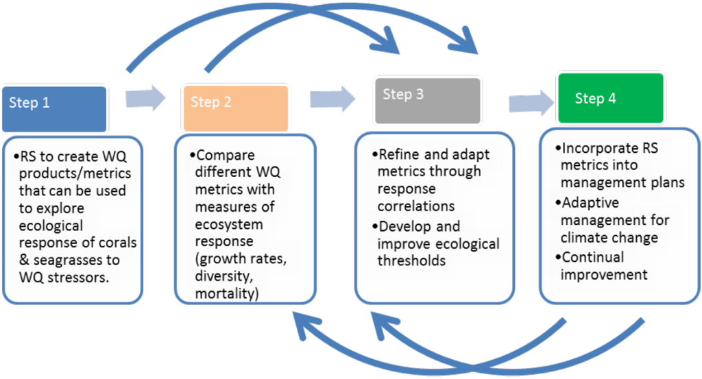
Figure 8. Adaptive strategy for the inclusion and use of RS products in the mapping and monitoring of GBR water quality and ecosystems.

Figure 8. Adaptive strategy for the inclusion and use of RS products in the mapping and monitoring of GBR water quality and ecosystems.

Research undertaken under the MMP water quality program has already initiated work with the modelling outputs of the GBR hydrodynamic model, but there are several other initiatives and outputs that are occurring in similar time-frames which offer potential opportunities to continue to extend our spatial and temporal understanding of water quality gradients in the GBR [53,70,88]. Modelling allows us to model what the reality would be under different scenarios and can provide integrated assessments that assess how different land management scenarios can influence the river plume condition and the GBR ecosystems. Utilising hydrodynamic and biogeochemical models in combination with ocean colour has been a key research area for international space agencies and ecosystem managers and can provide an important source of data for GBR managers [53,98,104].

4. Conclusions

Remote-sensed data can provide a useful and productive monitoring tool; however, the remote-sensed products need to be used with caution, dependent on the locations and optical conditions of the underlying water, due to uncertainties associated with Case 2 waters. Quantifying uncertainties inherent to the RS data for Level 1, 2 and 3 products, as well as with the in situ water quality and ecosystem health monitoring datasets, is crucial in determining how accurate the regionally-designed water quality products are, and in identifying the best data sets and information (or combination of information) sources to be used for the management of specific regions or seasons of the GBR. A fully functional monitoring program will need to adapt and integrate novel reporting methods to ensure consistency of reporting across large systems such as the GBR. The integration of data, from in situ to remote-sensed data and to validated hydrodynamic and biogeochemical models provides a challenging but comprehensive method to monitor, measure, and report on water quality in the GBR.

References

- Tol, R.; Klein, R.; Jansen, H.; Verbruggen, H. Some economic considerations on the importance of proactive integrated coastal zone management. Ocean Coast. Manag. 1996, 32, 39–55. [Google Scholar] [CrossRef]
- Delhez, É.J.; Barth, A. Science based management of coastal waters. J. Mar. Syst. 2011, 88, 1–2. [Google Scholar]
- Dickey, T. Studies of coastal ocean dynamics and processes using emerging optical technologies. Oceanography 2004, 17, 9–13. [Google Scholar] [CrossRef]
- Stock, C.A.; Alexander, M.A.; Bond, N.A.; Brander, K.M.; Cheung, W.W.; Curchitser, E.N.; Delworth, T.L.; Dunne, J.P.; Griffies, S.M.; Haltuch, M.A. On the use of IPCC-class models to assess the impact of climate on living marine resources. Prog. Oceanogr. 2011, 88, 1–27. [Google Scholar] [CrossRef]
- Doney, S.C. The growing human footprint on coastal and open-ocean biogeochemistry. Science 2010, 328, 1512–1516. [Google Scholar] [CrossRef] [PubMed]
- Ostendorf, B. Overview: Spatial information and indicators for sustainable management of natural resources. Ecol. Indic. 2011, 11, 97–102. [Google Scholar] [CrossRef]
- Brando, V.; Steven, A.; Schroeder, T.; Dekker, A.; Park, Y.; Daniel, P.; Ford, P. Remote-Sensing of GBR Waters to Assist Performance Monitoring of Water Quality Improvement Plans in Far North Queensland; Final Report for Department of the Environment and Water Heritage and the Arts; CSIRO Land & Water: Canberra, ACT, Australia, 2010; p. 88. [Google Scholar]
- International Ocean-Colour Coordinating Group (IOCCG). Remote Sensing of Ocean Colour in Coastal, and Other Optically-Complex, Waters; Sathyendranath, S., Ed.; Reports of the International Ocean-Colour Coordinating Group, No. 4; IOCCG: Dartmouth, NS, Canada, 2000; p. 50. [Google Scholar]
- International Ocean-Colour Coordinating Group (IOCCG). Guide to the Creation and Use of Ocean-Colour, Level-3, Binned Data Products; Antoine, D., Ed.; Reports of the International Ocean-Colour Coordinating Group, No. 4; IOCCG: Dartmouth, NS, Canada, 2004; p. 85. [Google Scholar]
- Waterhouse, J.; Brodie, J.; Lewis, S.; Mitchell, A. Quantifying the sources of pollutants in the Great Barrier Reef catchments and the relative risk to reef ecosystems. Mar. Pollut. Bull. 2012, 65, 394–406. [Google Scholar] [CrossRef] [PubMed]
- Kroon, F.J.; Kuhnert, P.M.; Henderson, B.L.; Wilkinson, S.N.; Kinsey-Henderson, A.; Abbott, B.; Brodie, J.E.; Turner, R.D. River loads of suspended solids, nitrogen, phosphorus and herbicides delivered to the Great Barrier Reef lagoon. Mar. Pollut. Bull. 2012, 65, 167–181. [Google Scholar] [CrossRef] [PubMed]
- Brodie, J.E.; Devlin, M.; Haynes, D.; Waterhouse, J. Assessment of the eutrophication status of the Great Barrier Reef lagoon (Australia). Biogeochemistry 2010, 106, 281–302. [Google Scholar] [CrossRef]
- McKenzie, L.; Collier, C.; Waycott, M. Reef Rescue Marine Monitoring Program: Inshore Seagrass; Annual Report for the Sampling Period 1st July 2011–31st May 2012; Tropwater, James Cook University: Cairns, QLD, Australia, 2014; p. 76. [Google Scholar]
- Thompson, A.; Schroeder, T.; Brando, V.E.; Schaffelke, B. Coral community responses to declining water quality: Whitsunday Islands, Great Barrier Reef, Australia. Coral Reefs 2014, 33, 923–938. [Google Scholar] [CrossRef]
- Johnson, J. Status of Marine and Coastal Assets in the Wet Tropics Region; Terrain: Cairns, QLD, Australia, 2015. [Google Scholar]
- Bell, I.; Ariel, E. Dietary shift in green turtles. Seagrass-Watch News 2011, 44, 2–5. [Google Scholar]
- McKenzie, L.J.; Yoshida, R.L.; Unsworth, R. Disturbance influences the invasion of a seagrass into an existing meadow. Mar. Pollut. Bull. 2014, 86, 186–196. [Google Scholar] [CrossRef] [PubMed]
- Anonymous. Great Barrier Reef Report Card 2012 and 2013: Reef Water Quality Protection Plan; Department of Premier and Cabinet, Reef Water Quality Protection Plan Secretariat: Brisbane, QLD, Australia, 2014. Available online: http://www.reefplan.qld.gov.au (accessed on 14 September 2015).
- Schaffelke, B.; Carleton, J.; Doyle, J.; Furnas, M.; Gunn, K.; Skuza, M.; Wright, M.; Zagorskis, I. Reef Rescue Marine Monitoring Program—Final Report of AIMS Activities 2010/11-Inshore Water Quality Monitoring; A Report for the Great Barrier Reef Marine Park Authority; Australian Institute of Marine Science: Townsville, QLD, Australia, 2001; p. 83.
- Kennedy, K.; Devlin, M.; Bentley, C.; Lee-Chue, K.; Paxman, C.; Carter, S.; Lewis, S.E.; Brodie, J.; Guy, E.; Vardy, S. The influence of a season of extreme wet weather events on exposure of the world heritage area Great Barrier Reef to pesticides. Mar. Pollut. Bull. 2012, 64, 1495–1507. [Google Scholar] [CrossRef] [PubMed]
- Johnson, J.; Brando, V.; Devlin, M.; McKenzie, L.; Morris, S.; Schaffelke, B.; Thompson, A.; Waterhouse, J.; Waycott, M. Reef Rescue Marine Monitoring Program: 2009/2010 Synthesis Report; Report for the Reef and Rainforest Research Centre Consortium of Monitoring Providers for the Great Barrier Reef Marine Park Authority; Reef and Rainforest Research Centre Limited: Cairns, QLD, Australia, 2011; p. 104. [Google Scholar]
- Devlin, M.; Wenger, A.; Da Silva, E.; Alvarez Romero, J.G.; Waterhouse, J.; McKenzie, L. Extreme weather conditions in the Great Barrier Reef: Drivers of change? In 21A Watershed Management and Reef Pollution, Proceedings of the 12th International Coral Reef Symposium, Cairns, QLD, Australia, 9–13 July 2012; ARC Centre of Excellence for Coral Reef Studies, James Cook University: Townsville, QLD, Australia, 2012. [Google Scholar]
- Devlin, M.; Waterhouse, J.; Taylor, J.; Brodie, J. Flood Plumes in the Great Barrier Reef: Spatial and Temporal Patterns in Composition and Distribution; A Report to Great Barrier Reef Marine Park Authority; TropWater, James Cook University: Townsville, QLD, Australia, 2001. [Google Scholar]
- Furnas, M.J.; Mitchell, A.W.; Skuza, M.S. River inputs of nutrients and sediment to the Great Barrier Reef. In Proceedings of State of the Great Barrier Reef World Heritage Area Workshop, Townsville, QLD, Australia, 27–29 November 1995; pp. 46–68.
- Mitchell, C.; Brodie, J.; White, I. Sediments, nutrients and pesticide residues in event flow conditions in streams of the Mackay Whitsunday Region, Australia. Mar. Pollut. Bull. 2005, 51, 23–36. [Google Scholar] [CrossRef] [PubMed]
- Wolanski, E.; Jones, M. Physical properties of Great Barrier Reef lagoon waters near Townsville. I. Effects of Burdekin River floods. Mar Freshw. Res. 1981, 32, 305–319. [Google Scholar] [CrossRef]
- Wolanski, E.; van Senden, D. Mixing of Burdekin river flood waters in the Great Barrier Reef. Mar Freshw. Res. 1983, 34, 49–63. [Google Scholar] [CrossRef]
- Álvarez-Romero, J.G.; Devlin, M.; Teixeira da Silva, E.; Petus, C.; Ban, N.C.; Pressey, R.L.; Kool, J.; Roberts, J.; Cerdeira, S.; Wenger, A.; et al. Following the flow: A combined remote sensing-GIS approach to model exposure of marine ecosystems to riverine flood plume. J. Environ. Manag. 2013, 119, 194–207. [Google Scholar] [CrossRef] [PubMed]
- Schroeder, T.; Devlin, M.J.; Brando, V.E.; Dekker, A.G.; Brodie, J.E.; Clementson, L.A.; McKinna, L. Inter-annual variability of wet season freshwater plume extent into the Great Barrier Reef lagoon based on satellite coastal ocean colour observations. Mar. Pollut. Bull. 2012, 65, 210–223. [Google Scholar] [CrossRef] [PubMed]
- Devlin, M.J.; da Silva, E.; Petus, C.; Wenger, A.; Zeh, D.; Tracey, D.; Álvarez-Romero, J.G.; Brodie, J. Combining in situ water quality and remotely sensed data across spatial and temporal scales to measure variability in wet season chlorophyll-a: Great Barrier Reef lagoon (Queensland, Australia). Ecol. Proc. 2013, 2. [Google Scholar] [CrossRef]
- Devlin, M.J.; Álvarez-Romero, J.; da Silva, E.T.; DeBose, J.; Petus, C.; Wenger, A. Reef Rescue Marine Monitoring Program; Final Report of JCU Activities 2011/12-Flood Plumes and Extreme Weather Monitoring for the Great Barrier Reef Marine Park Authority; TropWater, James Cook University: Townsville, QLD, Australia, 2013; p. 116. [Google Scholar]
- Devlin, M.; Schaffelke, B. Spatial extent of riverine flood plumes and exposure of marine ecosystems in the Tully coastal region, Great Barrier Reef. Mar. Freshw. Res. 2009, 60, 1109–1122. [Google Scholar] [CrossRef]
- Petus, C.; da Silva, E.T.; Devlin, M.; Wenger, A.S.; Álvarez-Romero, J.G. Using MODIS data for mapping of water types within river plumes in the Great Barrier Reef, Australia: Towards the production of river plume risk maps for reef and seagrass ecosystems. J. Environ. Manag. 2014, 137, 163–177. [Google Scholar] [CrossRef] [PubMed]
- Devlin, M.; Petus, C.; da Silva, E.; Alvarez-Romero, J.G.; Zeh, D.; Waterhouse, J.; Brodie, J. Chapter 5: Mapping of exposure to flood plumes, water types and exposure to pollutants (DIN, TSS) in the Great Barrier Reef: Toward the production of operational risk maps for the World’s most iconic marine ecosystem. In Assessment of the Relative Risk of Water Quality to Ecosystems of the Great Barrier Reef: Supporting Studies; A Report to the Department of the Environment and Heritage Protection, Queensland Government, Brisbane, TropWATER Report 13/30; TropWater, James Cook University: Townsville, QLD, Australia, 2013; pp. 152–175. [Google Scholar]
- Devlin, M.J.; McKinna, L.W.; Alvarez-Romero, J.G.; Petus, C.; Abott, B.; Harkness, P.; Brodie, J. Mapping the pollutants in surface riverine flood plume waters in the Great Barrier Reef, Australia. Mar. Pollut. Bull. 2012, 65, 224–235. [Google Scholar] [CrossRef] [PubMed]
- Brando, V.E.; Dekker, A.G.; Park, Y.J.; Schroeder, T. Adaptive semianalytical inversion of ocean color radiometry in optically complex waters. Appl. Opt. 2012, 51, 2808–2833. [Google Scholar] [CrossRef] [PubMed]
- Brando, V.; Schroeder, T.; Dekker, A.; Park, Y. Reef Rescue Marine Monitoring Program: Using Remote Sensing for GBR Wide Water Quality; Final Report for 2009/10 Activities; CSIRO Land & Water: Brisbane, QLD, Australia, 2010. [Google Scholar]
- Devlin, M.J.; Brodie, J. Terrestrial discharge into the Great Barrier Reef Lagoon: Nutrient behavior in coastal waters. Mar. Pollut. Bull. 2005, 51, 9–22. [Google Scholar] [CrossRef] [PubMed]
- Petus, C.; Collier, C.; Devlin, M.; Rasheed, M.; McKenna, S. Using MODIS data for understanding changes in seagrass meadow health: A case study in the Great Barrier Reef (Australia). Mar. Environ. Res. 2014, 98, 68–85. [Google Scholar] [CrossRef] [PubMed]
- Klemas, V. Airborne remote sensing of coastal features and processes: An overview. J. Coast. Res. 2012, 29, 239–255. [Google Scholar] [CrossRef]
- Clarke, K.R.; Warwick, R.M. Change in Marine Communities: An Approach to Statistical Analysis and Interpretation; Plymouth Routines In Multivariate Ecological Research (PRIMER-E): Plymouth, UK, 1994. [Google Scholar]
- Morel, A.; Gentili, B.; Chami, M.; Ras, J. Bio-optical properties of high chlorophyll Case 1 waters and of yellow-substance-dominated Case 2 waters. Deep Sea Res. Part I: Oceanogr. Res. Pap. 2006, 53, 1439–1459. [Google Scholar] [CrossRef]
- Morel, A.; Prieur, L. Analysis of variations in ocean color. Limnol. Oceanogr. 1977, 22, 709–722. [Google Scholar] [CrossRef]
- McClain, C.R. A decade of satellite ocean color observations. Annu. Rev. Mar. Sci. 2009, 1, 19–42. [Google Scholar] [CrossRef] [PubMed]
- Phinn, S.; Dekker, A.; Brando, V.E.; Roelfsema, C. Mapping water quality and substrate cover in optically complex coastal and reef waters: An integrated approach. Mar. Pollut. Bull. 2005, 51, 459–469. [Google Scholar] [CrossRef] [PubMed]
- Schaffelke, B.; Carleton, J.; Skuza, M.; Zagorskis, I.; Furnas, M.J. Water quality in the inshore Great Barrier Reef lagoon: Implications for long-term monitoring and management. Mar. Pollut. Bull. 2012, 65, 249–260. [Google Scholar] [CrossRef] [PubMed]
- Bentley, C.; Devlin, M.; Paxman, C.; Chue, K.L.; Mueller, J.F. Pesticide Monitoring in Inshore Waters of the Great Barrier Reef Using both Time-Integrated and Event Monitoring Techniques (2011–2012); The National Research Centre for Environmental Toxicology (Entox), The University of Queensland: Brisbane, QLD, Australia, 2012; p. 91. [Google Scholar]
- Devlin, M.; Schroeder, T.; McKinna, L.; Brodie, J.; Brando, V.; Dekker, A. Monitoring and mapping of flood plumes in the Great Barrier Reef based on in situ and remote sensing observations. In Advances in Environmental Remote Sensing to Monitor Global Changes; CRC Press: Boca Raton, FL, USA, 2011; pp. 147–191. [Google Scholar]
- Lewis, S.E.; Brodie, J.E.; Bainbridge, Z.T.; Rohde, K.W.; Davis, A.M.; Masters, B.L.; Maughan, M.; Devlin, M.J.; Mueller, J.F.; Schaffelke, B. Herbicides: A new threat to the Great Barrier Reef. Environ. Pollut. 2009, 157, 2470–2484. [Google Scholar] [CrossRef] [PubMed]
- Brodie, J.E.; Kroon, F.J.; Schaffelke, B.; Wolanski, E.C.; Lewis, S.E.; Devlin, M.J.; Bohnet, I.C.; Bainbridge, Z.T.; Waterhouse, J.; Davis, A.M. Terrestrial pollutant runoff to the Great Barrier Reef: An update of issues, priorities and management responses. Mar. Pollut. Bull. 2012, 65, 81–100. [Google Scholar] [CrossRef] [PubMed]
- Kennedy, K.; Schroeder, T.; Shaw, M.; Haynes, D.; Lewis, S.; Bentley, C.; Paxman, C.; Carter, S.; Brando, V.E.; Bartkow, M.; et al. Long term monitoring of photosystem II Herbicides. Correlation with remotely sensed freshwater extent to monitor changes in the quality of water entering the Great Barrier Reef, Australia. Mar. Pollut. Bull. 2012, 65, 292–305. [Google Scholar] [CrossRef] [PubMed]
- Devlin, M.; DeBose, J.; Adjani, P.; Brodie, J. Chapter 8: Analysis of phytoplankton community structure in flood events in the Great Barrier Reef. In Assessment of the Relative Risk of Water Quality to Ecosystems of the Great Barrier Reef: Supporting Studies; A Report to the Department of the Environment and Heritage Protection, Queensland Government, Brisbane, TropWater Report 13/30; TropWater, James Cook University: Townsville, QLD, Australia, 2013; pp. 216–219. [Google Scholar]
- Brinkman, R.; Tonin, H.; Furnas, M.; Schaffelke, B.; Fa, F. Targeted Analysis of the Linkages between River Runoff and Risks for Crown-of-Thorns Starfish Outbreaks in the Northern GBR. Report for Terrain Natural Resource Management (NRM). Available online: http://www.terrain.org.au/Projects/Water-Quality-Improvement-Plan/Studies-and-Reports (accessed on 23 Steptember 2015).
- Waterhouse, J. (Compiler) Assessment of the Relative Risk of Water Quality to Ecosystems of the Great Barrier Reef: Supporting Studies; A Report to the Department of the Environment and Heritage Protection, Queensland Government; TropWATER Report 13/30; TropWater, James Cook University: Townsville, QLD, Australia, 2013; p. 229.
- King, B.; McAllister, F.; Wolanski, E.; Done, T.; Spagnol, S. River plume dynamics in the central Great Barrier Reef. In Oceanographic Processes of Coral Reefs: Physical and Biological Links in the Great Barrier Reef; CRC Press: Boca Raton, FL, USA, 2001; pp. 145–159. [Google Scholar]
- Parkinson, C.; Ward, A.; King, M. Earth Science Reference Handbook: A Guide to NASA’s Earth Science Program and Earth Observing Satellite Missions. National Aeronautics Space Administration. Available online: http://atrain.nasa.gov/publications/2006ReferenceHandbook.pdf (accessed on 24 September 2015).
- Brando, V.; Keen, R.; Daniel, P.; Baumeister, A.; Nethery, M.; Baumeister, H.; Hawdon, A.; Swan, G.; Mitchell, R.; Campbell, S. The Lucinda Jetty coastal observatory’s role in satellite ocean colour calibration and validation for Great Barrier Reef coastal waters. In Proceedings of IEEE OCEANS Conference, Frascati, Italy, 17–19 March 2010; pp. 1–8.
- King, E.A.; Schroeder, T.; Brando, V.E.; Super, K. A Pre-Operational System for Satellite Monitoring of Great Barrier Reef Marine Water Quality; Wealth from Oceans Flagship Report; CSIRO Land & Water: Canberra, ACT, Australia, 2013; p. 56. [Google Scholar]
- Weeks, S.; Werdell, P.; Schaffelke, B.; Canto, M.; Lee, Z.; Wilding, J.; Feldman, G. Satellite-derived photic depth on the Great Barrier Reef: Spatio-temporal patterns of water clarity. Remote Sens. 2012, 4, 3781–3795. [Google Scholar] [CrossRef]
- Schroeder, T.; Behnert, I.; Schaale, M.; Fischer, J.; Doerffer, R. Atmospheric correction algorithm for MERIS above Case-2 waters. Int. J. Remote Sens. 2007, 28, 1469–1486. [Google Scholar] [CrossRef]
- Fabricius, K.E.; Logan, M.; Weeks, S.; Brodie, J. The effects of river run-off on water clarity across the central Great Barrier Reef. Mar. Pollut. Bull. 2014, 84, 191–200. [Google Scholar] [CrossRef] [PubMed]
- Petus, C.; Da Silva, E.; Devlin, M.; Tracey, D.; Woolf, N. Mapping Concentrations and Risk of Photosystem II Inhibiting Herbicide (PSII) Using Remote Sensing and Hydrodynamic Models: A Case Study in the Tully River Plume Waters, Queensland (Australia); TropWater Report; James Cook University: Townsville, QLD, Australia, 2015; p. 35. [Google Scholar]
- Petus, C.; Devlin, M.; da Silva, E.; Wenger, A.; Tracey, D. Estimating water clarity from optically active constituents along optical water quality gradients: A case study in the Great Barrier Reef River plume waters. In Presented at the Marine Monitoring Workshop, Townsville, QLD, Australia, 20 September 2014.
- Brodie, J.; Waterhouse, J.; Maynard, J.; Bennett, J.; Furnas, M.; Devlin, M.; Lewis, S.; Collier, C.; Schaffelke, B.; Fabricius, K. Assessment of the Relative Risk of Water Quality to Ecosystems of the Great Barrier Reef; A Report to the Department of the Environment and Heritage Protection, Queensland Government, Brisbane, TropWATER Report 13/28; TropWater, James Cook University: Townsville, QLD, Australia, 2013; p. 58. [Google Scholar]
- Devlin, M.; Petus, C.; Collier, C.; Zeh, D.; McKenzie, L. Chapter 6: Seagrass and water quality impacts including a case study linking annual measurements of seagrass change against satellite water clarity data (Cleveland Bay). In Assessment of the Relative Risk of Water Quality to Ecosystems of the Great Barrier Reef: Supporting Studies; A Report to the Department of the Environment and Heritage Protection, Queensland Government, Brisbane, TropWATER Report 13/30; TropWater, James Cook University: Townsville, QLD, Australia, 2013; pp. 175–198. [Google Scholar]
- Fabricius, K.E.; Okaji, K.; De’ath, G. Three lines of evidence to link outbreaks of the crown-of-thorns seastar Acanthaster planci to the release of larval food limitation. Coral Reefs 2010, 29, 593–605. [Google Scholar] [CrossRef]
- Van Dam, J.; Uthicke, S.; Beltran, V.; Mueller, J.; Negri, A. Combined thermal and herbicide stress in functionally diverse coral symbionts. Environ. Pollut. 2015, 204, 271–279. [Google Scholar] [CrossRef] [PubMed]
- Petus, C.; Devlin, M.; da Silva, E.; Wolff, N.; Tracey, D.; Brodie, J. Risk from the Exposure of Coral Reefs and Seagrass Beds to Land-Sourced Contaminants in River Flood Plumes of the Great Barrier Reef: Validating a Simplified Satellite Framework with Environmental Data; TropWATER Report; James Cook University: Townsville, QLD, Australia, 2015; p. 25. [Google Scholar]
- Brodie, J.; Waterhouse, J.; Maynard, J. Assessment of the Relative Risk of Degraded Water Quality to Ecosystems of the Great Barrier Reef; A Report to the Department of the Environment and Heritage Protection, TropWATER Report 13/28; James Cook University: Townsville, QLD, Australia, 2015. [Google Scholar]
- Furnas, M.; Brinkman, R.; Fabricius, K.; Tonin, H.; Schaffelke, B. Linkages between river runoff, phytoplankton blooms and primary outbreaks of crown-of-thorns starfish in the Northern GBR. In Assessment of the Relative Risk of Water Quality to Ecosystems of the Great Barrier Reef: Supporting Studies; A Report to the Department of the Environment and Heritage Protection, Queensland Government, Brisbane, TropWATER Report 13/30; TropWater, James Cook University: Townsville, QLD, Australia, 2013; pp. 4–38. [Google Scholar]
- Moderate Resolution Imaging Spectroradiometer. Available online: http://modis.gsfc.nasa.gov/ (accessed on 18 September 2015).
- Baith, K.; Lindsay, R.; Fu, G.; McClain, C.R. Data analysis system developed for ocean color satellite sensors. Eos, Trans. Am. Geophys. Union 2001, 82, 202. [Google Scholar] [CrossRef]
- Australian Government, Bureau of Meteorology. Available online: http://www.bom.gov.au/marinewaterquality/ (accessed on 18 September 2105).
- Sweatman, H.; Delean, S.; Syms, C. Assessing loss of coral cover on Australia’s Great Barrier Reef over two decades, with implications for longer-term trends. Coral Reefs 2011, 30, 521–531. [Google Scholar] [CrossRef]
- Sweatman, H.H.; Cheal, A.A.; Coleman, G.G.; Delean, S.S.; Fitzpatrick, B.B.; Miller, I.I.; Ninio, R.R.; Osborne, K.K.; Page, C.C.; Thompson, A.A. Long-Term Monitoring of the Great Barrier Reef; Status Report Number 5; Australian Institute of Marine Science: Cape Ferguson, QLD, Australian, 2001; p. 106.
- Bainbridge, Z.T.; Wolanski, E.; Alvarez-Romero, J.G.; Lewis, S.E.; Brodie, J.E. Fine sediment and nutrient dynamics related to particle size and floc formation in a Burdekin River flood plume, Australia. Mar. Pollut. Bull. 2012, 65, 236–248. [Google Scholar] [CrossRef] [PubMed]
- Petus, C.; Devlin, M.; Da Silva, E.; Brodie, J. Assessing Uncertainty in Chlorophyll a Assessments from Remote Sensing in the GBR; TropWater, James Cook University: Townsville, QLD, Australia, 2015; p. 55. [Google Scholar]
- Lewis, S.E.; Olley, J.; Furuichi, T.; Sharma, A.; Burton, J. Complex sediment deposition history on a wide continental shelf: Implications for the calculation of accumulation rates on the Great Barrier Reef. Earth Planet. Sci. Lett. 2014, 393, 146–158. [Google Scholar] [CrossRef]
- DNRM. State of Queensland, Australia. Department of Natural Resources and Mines “Watershed”. Available online: http://www.derm.qld.gov.au/watershed/index.html (accessed on 1 September 2015).
- Kroon, F.J. Towards ecologically relevant targets for river pollutant loads to the Great Barrier Reef. Mar. Pollut. Bull. 2012, 65, 261–266. [Google Scholar] [CrossRef] [PubMed]
- Lewis, S.; Brodie, J.; Endo, G.; Lough, J.; Furnas, M.; Bainbridge, Z. Synthesizing Historical Land Use Change, Fertiliser and Pesticide Usage and Pollutant Load Data in the Regulated Catchments to Quantify Baseline and Changing Loads Exported to the Great Barrier Reef; TropWATER Report 14; James Cook University: Townsville, QLD, Australia, 2015; p. 35. [Google Scholar]
- Brodie, J.; Burford, M.; Davis, A.; da Silva, E.; Devlin, M.; Furnas, M.; Kroon, F.; Lewis, S.; Lønborg, C.; O’Brien, D. The Relative Risks to Water Quality from Particulate Nitrogen Discharged from Rivers to the Great Barrier Reef in Comparison to Other Forms of Nitrogen; TropWATER Report 14/31; James Cook University: Townsville, QLD, Australia, 2015; p. 55. [Google Scholar]
- Collier, C.; Devlin, M.; Langlois, L.; Petus, C.; McKenzie, L.; Waycott, M. Thresholds and Indicators of Declining Water Quality as Tools for Tropical Seagrass Management; Reef and Rainforest Research Centre: Cairns, QLD, Australia, 2014; p. 93. [Google Scholar]
- Lahr, J.; Kooistra, L. Environmental risk mapping of pollutants: State of the art and communication aspects. Sci. Total Environ. 2010, 408, 3899–3907. [Google Scholar] [CrossRef] [PubMed]
- Wooldridge, S.A. Water quality and coral bleaching thresholds: formalising the linkage for the inshore reefs of the Great Barrier Reef, Australia. Mar. Pollut. Bull. 2009, 58, 745–751. [Google Scholar] [CrossRef] [PubMed]
- Brodie, J.; Fabricius, K.; De’ath, G.; Okaji, K. Are increased nutrient inputs responsible for more outbreaks of crown-of-thorns starfish? An appraisal of the evidence. Mar. Pollut. Bull. 2005, 51, 266–278. [Google Scholar] [CrossRef] [PubMed]
- Uthicke, S.; Logan, M.; Liddy, M.; Francis, D.; Hardy, N.; Lamare, M. Climate change as an unexpected co-factor promoting coral eating seastar (Acanthaster planci) outbreaks. Sci. Rep. 2015. [Google Scholar] [CrossRef] [PubMed]
- Mumby, P.J.; Anthony, K. Resilience metrics to inform ecosystem management under global change with application to coral reefs. Methods Ecol. Evol. 2015. [Google Scholar] [CrossRef]
- Magnusson, M.; Heimann, K.; Ridd, M.; Negri, A.P. Chronic herbicide exposures affect the sensitivity and community structure of tropical benthic microalgae. Mar. Pollut. Bull. 2012, 65, 363–372. [Google Scholar] [CrossRef] [PubMed]
- Fabricius, K.E.; Cooper, T.F.; Humphrey, C.; Uthicke, S.; De’ath, G.; Davidson, J.; LeGrand, H.; Thompson, A.; Schaffelke, B. A bioindicator system for water quality on inshore coral reefs of the Great Barrier Reef. Mar. Pollut. Bull. 2012, 65, 320–332. [Google Scholar] [CrossRef] [PubMed]
- Brodie, J.; Waterhouse, J. A critical review of environmental management of the “not so Great” Barrier Reef. Est. Coast Shelf Sci. 2012, 104, 1–22. [Google Scholar] [CrossRef]
- Brodie, J.; Mitchell, A.; Furnas, M.; Haynes, D.; Waterhouse, J.; Ghonim, S.; Morris, S.; Yorkston, H.; Audas, D. Developing catchment pollutant load targets for the protection of the Great Barrier Reef. In Proceedings of the 2nd National Conference on Aquatic Environments: Sustaining our Aquatic Environments—Implementing Solutions, Townsville, QLD, Australia, 20–23 November 2001.
- Fabricius, K.E. Effects of terrestrial runoff on the ecology of corals and coral reefs: Review and synthesis. Mar. Pollut. Bull. 2005, 50, 125–146. [Google Scholar] [CrossRef] [PubMed]
- Fabricius, K.E.; De’ath, G.; Humphrey, C.; Zagorskis, I.; Schaffelke, B. Intra-annual variation in turbidity in response to terrestrial runoff on near-shore coral reefs of the Great Barrier Reef. Estuar. Coast. Shelf Sci. 2013, 116, 57–65. [Google Scholar] [CrossRef]
- Bartley, R.; Bainbridge, Z.T.; Lewis, S.E.; Kroon, F.J.; Wilkinson, S.N.; Brodie, J.E.; Silburn, D.M. Relating sediment impacts on coral reefs to watershed sources, processes and management: A review. Sci. Total Environ. 2014, 468, 1138–1153. [Google Scholar] [CrossRef] [PubMed]
- Brown, C.J.; Saunders, M.I.; Possingham, H.P.; Richardson, A.J. Interactions between global and local stressors of ecosystems determine management effectiveness in cumulative impact mapping. Divers. Distrib. 2014, 20, 538–546. [Google Scholar] [CrossRef]
- Grech, A.; Chartrand-Miller, K.; Erftemeijer, P.; Fonseca, M.; McKenzie, L.; Rasheed, M.; Taylor, H.; Coles, R. A comparison of threats, vulnerabilities and management approaches in global seagrass bioregions. Environ. Res. Lett. 2012, 7, 024006. [Google Scholar] [CrossRef]
- Anthony, K.; Dambacher, J.; Walshe, T.; Beeden, R. A Framework for Understanding Cumulative Impacts, Supporting Environmental Decisions and Informing Resilience Based Management of the Great Barrier Reef World Heritage Area; Final Report to the Great Barrier Reef Marine Park Authority and Department of the Environment; GBRMPA: Townsville, QLD, Australia, 2013.
- Anthony, K.; Marshall, P.A.; Abdulla, A.; Beeden, R.; Bergh, C.; Black, R.; Eakin, C.M.; Game, E.T.; Gooch, M.; Graham, N.A. Operationalizing resilience for adaptive coral reef management under global environmental change. Glob. Change Biol. 2015, 21, 48–61. [Google Scholar] [CrossRef] [PubMed]
- Elmhirst, T.; Connolly, S.R.; Hughes, T.P. Connectivity, regime shifts and the resilience of coral reefs. Coral Reefs 2009, 28, 949–957. [Google Scholar] [CrossRef]
- Brodie, J.; Schroeder, T.; Rohde, K.; Faithful, J.; Masters, B.; Dekker, A.; Brando, V.; Maughan, M. Dispersal of suspended sediments and nutrients in the Great Barrier Reef lagoon during river-discharge events: Conclusions from satellite remote sensing and concurrent flood-plume sampling. Mar. Freshw. Res. 2010, 61, 651–664. [Google Scholar] [CrossRef]
- Brodie, J.; Lewis, S.; Wooldridge, S.; Bainbridge, Z.; Kroon, F. Ecologically Relevant Targets for Pollutant Discharge from the Drainage Basins of the Wet Tropics Region; A Report for Centre for Tropical Water & Aquatic Ecosystem Research (TropWATER), TropWATER Report 14/33; James Cook University: Townsville, QLD, Australia, 2014; p. 47. [Google Scholar]
- Martin, K.C.; McKenzie, L.J.; Thompson, A.; Muller, J.; Bentley, C.; Paxman, C.; Collier, C.; Waycott, M.; Brando, V.; Devlin, M.; et al. Reef Rescue Marine Monitoring Program Synthesis Report. 2010–2011; GBRMPA: Townsville, QLD, Australia. Available online: http://elibrary.gbrmpa.gov.au/jspui/handle/11017/2931 (accessed on 23 September 2015).
- Maynard, J.A.; Beeden, R.; Puotinen, M.; Johnson, J.E.; Marshall, P.; Hooidonk, R.; Heron, S.F.; Devlin, M.; Lawrey, E.; Dryden, J. Great Barrier Reef no-take areas include a range of disturbance regimes. Conserv. Lett. 2015. [Google Scholar] [CrossRef]
- Blondeau-Patissier, D.; Schroeder, T.; Brando, V.E.; Maier, S.W.; Dekker, A.G.; Phinn, S. ESA-MERIS 10-year mission reveals contrasting phytoplankton bloom dynamics in two tropical regions of Northern Australia. Remote Sens. 2014, 6, 2963–2988. [Google Scholar] [CrossRef]
- Blondeau-Patissier, D.; Brando, V.; Dekker, A.; Phinn, S.; Weeks, S.; Schroeder, T.; Park, Y.-J. Phytoplankton response to episodic events and long-term trends in the Great Barrier Reef lagoonal waters: towards a regional characterization. In Proceedings of the 20th Ocean Optics Conference (Ocean Optics XX), Anchorage, AL, USA, 25 September–1 October 2010.
- Brodie, J.; Lewis, S. Ecologically Relevant Targets for Pollutant Discharge from the Drainage Basins of the Burnett Mary Region Region, Great Barrier Reef; A Report for the Centre for Tropical Water & Aquatic Ecosystem Research (TropWATER), TropWATER Report 14/32; James Cook University: Townsville, QLD, Australia, 2014; p. 41. [Google Scholar]
- Waterhouse, J.; Brodie, J.; Tracey, D.; Lewis, S.; Hateley, L.; Brinkman, R.; Furnas, M.; Wolff, N.; da Silva, E.; O’Brien, D.; et al. Assessment of the Relative Risk of Water Quality to Ecosystems of the Wet Tropics Region, Great Barrier Reef; A Report to Terrain NRM, Innisfail; TropWATER Report 14/27; TropWATER, James Cook University: Townsville, QLD, Australia, 2014; p. 70. [Google Scholar]
- De’ath, G.; Fabricius, K.E.; Sweatman, H.; Puotinen, M. The 27-year decline of coral cover on the Great Barrier Reef and its causes. Natl. Acad. Sci. 2012, 109, 17995–17999. [Google Scholar] [CrossRef] [PubMed]
- Wolfe, K.; Graba-Landry, A.; Dworjanyn, S.A.; Byrne, M. Larval starvation to satiation: Influence of nutrient regime on the success of Acanthaster planci. PLoS One 2015, 10, e0122010. [Google Scholar] [CrossRef] [PubMed]
© 2015 by the authors; licensee MDPI, Basel, Switzerland. This article is an open access article distributed under the terms and conditions of the Creative Commons Attribution license (http://creativecommons.org/licenses/by/4.0/).