
Developing in situ Non-Destructive Estimates of Crop Biomass to Address Issues of Scale in Remote Sensing


Abstract
:
1. Introduction
2. Material and Methods
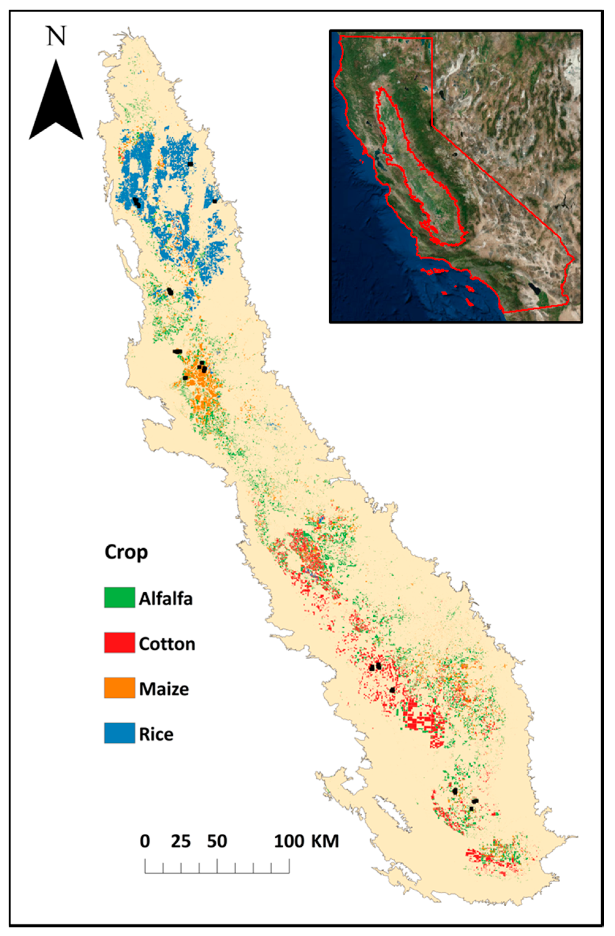
2.1. Study Area
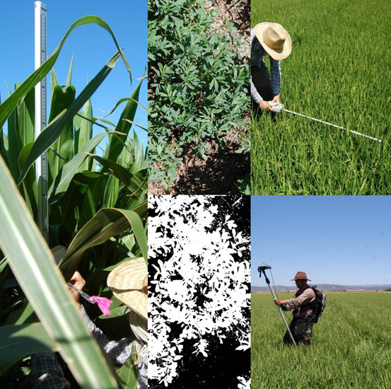
2.2. Non-Spectral Measurements and Processing

| Parameter | Crop Stage | Statistic | Alfalfa (N = 136) | Cotton (N = 147) | Maize (N = 151) | Rice (N = 106) |
|---|---|---|---|---|---|---|
| AWB | Sprouting | μ | 1984 | 776 | 7558 | 774 |
| (g∙m−2) | σ | 2517 | 757 | 3882 | 589 | |
| Flowering | μ | 16132 | 8134 | 13959 | 2703 | |
| σ | 12945 | 4025 | 2810 | 1089 | ||
| Senescence | μ | - | 9447 | 11857 | 2727 | |
| σ | - | 5770 | 3460 | 1133 | ||
| H | Sprouting | μ | 20.92 | 31.30 | 173.74 | 34.46 |
| σ | 13.65 | 10.38 | 87.07 | 14.50 | ||
| Flowering | μ | 51.41 | 98.21 | 292.18 | 77.36 | |
| σ | 14.00 | 16.67 | 29.47 | 12.72 | ||
| Senescence | μ | - | 103.13 | 316.39 | 79.82 | |
| σ | - | 20.03 | 22.56 | 15.71 | ||
| LAI | Sprouting | μ | 0.77 | 0.98 | 3.77 | 0.93 |
| σ | 1.09 | 0.88 | 1.86 | 1.43 | ||
| Flowering | μ | 3.89 | 4.18 | 5.49 | 3.86 | |
| σ | 1.63 | 1.78 | 1.63 | 1.68 | ||
| Senescence | μ | - | 3.62 | 3.99 | 4.86 | |
| σ | - | 1.76 | 1.01 | 1.13 | ||
| β | Sprouting | μ | 0.74 | 0.72 | 0.19 | 0.78 |
| σ | 0.26 | 0.18 | 0.18 | 0.25 | ||
| Flowering | μ | 0.15 | 0.15 | 0.05 | 0.15 | |
| σ | 0.14 | 0.16 | 0.06 | 0.13 | ||
| Senescence | μ | - | 0.21 | 0.08 | 0.05 | |
| σ | - | 0.19 | 0.07 | 0.06 | ||
| EXG | Sprouting | μ | 0.61 | 0.67 | 0.58 | 0.54 |
| σ | 0.12 | 0.14 | 0.25 | 0.29 | ||
| Flowering | μ | 0.81 | 0.71 | 0.54 | 0.82 | |
| σ | 0.26 | 0.10 | 0.32 | 0.09 | ||
| Senescence | μ | - | 0.59 | 0.53 | 0.60 | |
| σ | - | 0.22 | 0.32 | 0.06 | ||
| EXGR | Sprouting | μ | 0.24 | 0.21 | 0.51 | 0.34 |
| σ | 0.20 | 0.09 | 0.17 | 0.17 | ||
| Flowering | μ | 0.72 | 0.45 | 0.40 | 0.58 | |
| σ | 0.14 | 0.12 | 0.16 | 0.12 | ||
| Senescence | μ | - | 0.33 | 0.25 | 0.13 | |
| σ | - | 0.15 | 0.17 | 0.10 | ||
| NDI | Sprouting | μ | 0.48 | 0.56 | 0.51 | 0.45 |
| σ | 0.14 | 0.14 | 0.19 | 0.21 | ||
| Flowering | μ | 0.79 | 0.58 | 0.52 | 0.68 | |
| σ | 0.09 | 0.10 | 0.13 | 0.12 | ||
| Senescence | μ | - | 0.53 | 0.40 | 0.34 | |
| σ | - | 0.23 | 0.21 | 0.08 | ||
| meanG | Sprouting | μ | 0.34 | 0.34 | 0.37 | 0.35 |
| σ | 0.03 | 0.03 | 0.03 | 0.03 | ||
| Flowering | μ | 0.41 | 0.34 | 0.35 | 0.39 | |
| σ | 0.03 | 0.03 | 0.03 | 0.05 | ||
| Senescence | μ | - | 0.33 | 0.33 | 0.30 | |
| σ | - | 0.03 | 0.03 | 0.02 | ||
| medianG | Sprouting | μ | 0.38 | 0.38 | 0.41 | 0.37 |
| σ | 0.03 | 0.04 | 0.04 | 0.05 | ||
| Flowering | μ | 0.45 | 0.39 | 0.38 | 0.44 | |
| σ | 0.02 | 0.04 | 0.05 | 0.04 | ||
| Senescence | μ | - | 0.36 | 0.36 | 0.34 | |
| σ | - | 0.03 | 0.04 | 0.04 |
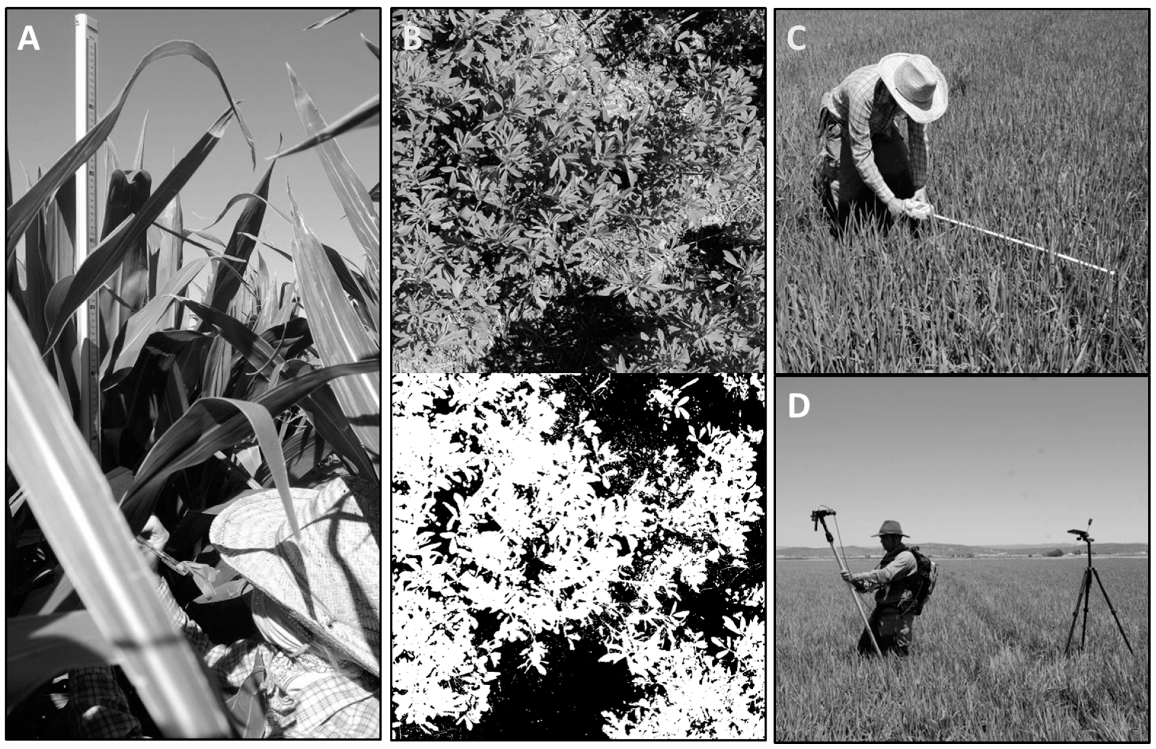
2.2.1. Fraction of Vegetation Cover (FVC)
2.2.2. Gap Fraction (β) and Leaf Area Index (LAI)
2.3. Spectral Measurements and Processing
2.3.1. Hyperspectral Data Transformations
2.3.2. Data Reduction for Model-building
2.4. Model Building
2.4.1. Multiple-Band Vegetation Index (MBVI)
2.4.2. Two-Band Vegetation Index (TBVI)
2.4.3. Hyperspectral Narrowband versus Broadband Predictors
2.5. Model Validation
3. Results
3.1. Non-Spectral Measurement Summary
3.2. Spectral Measurement Summary


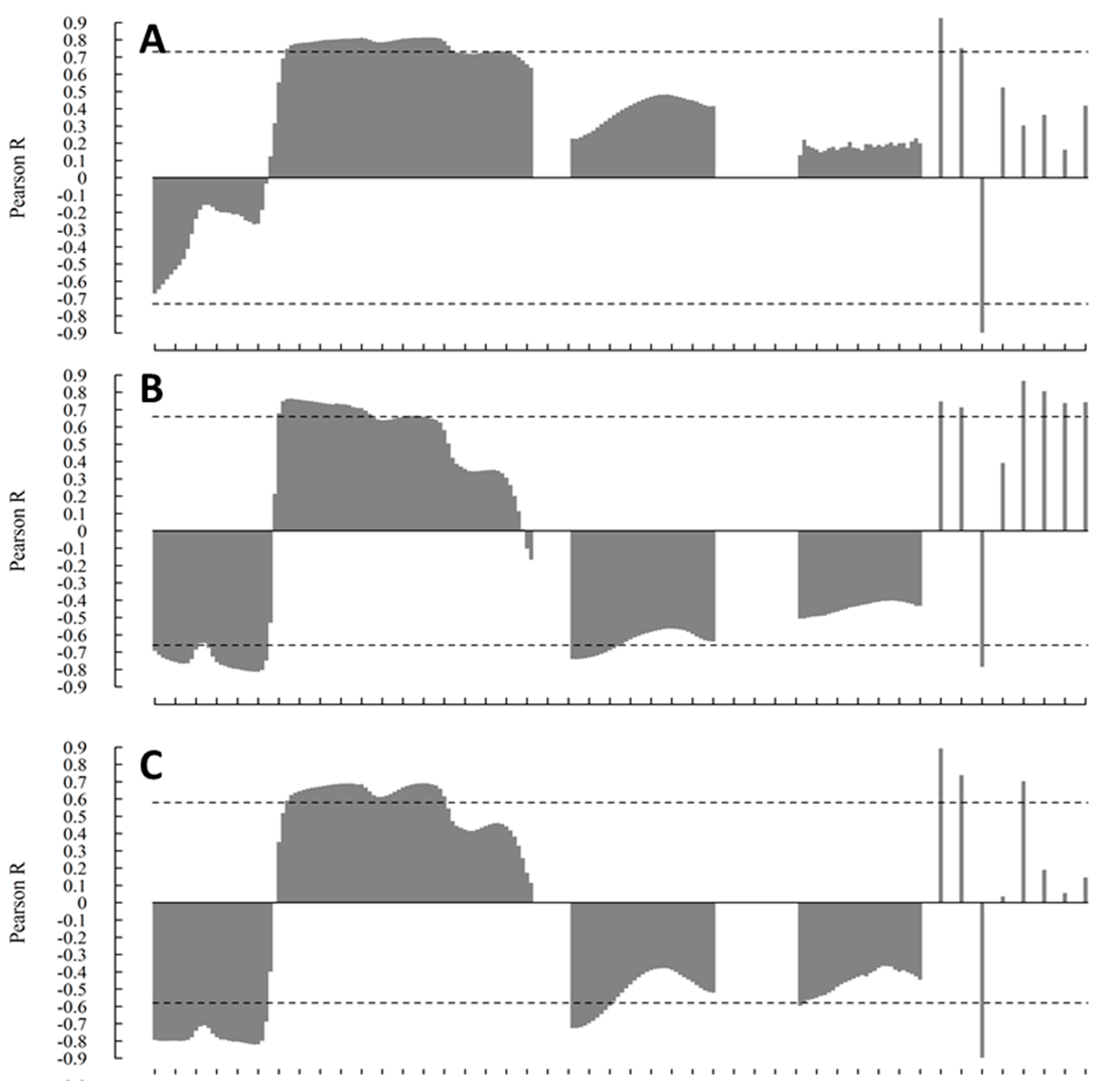
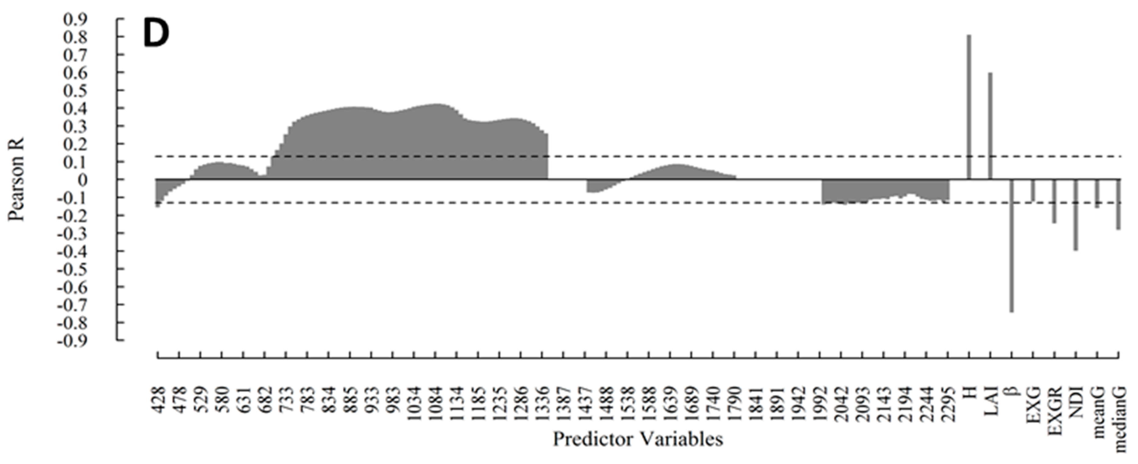
3.3. Model-Building
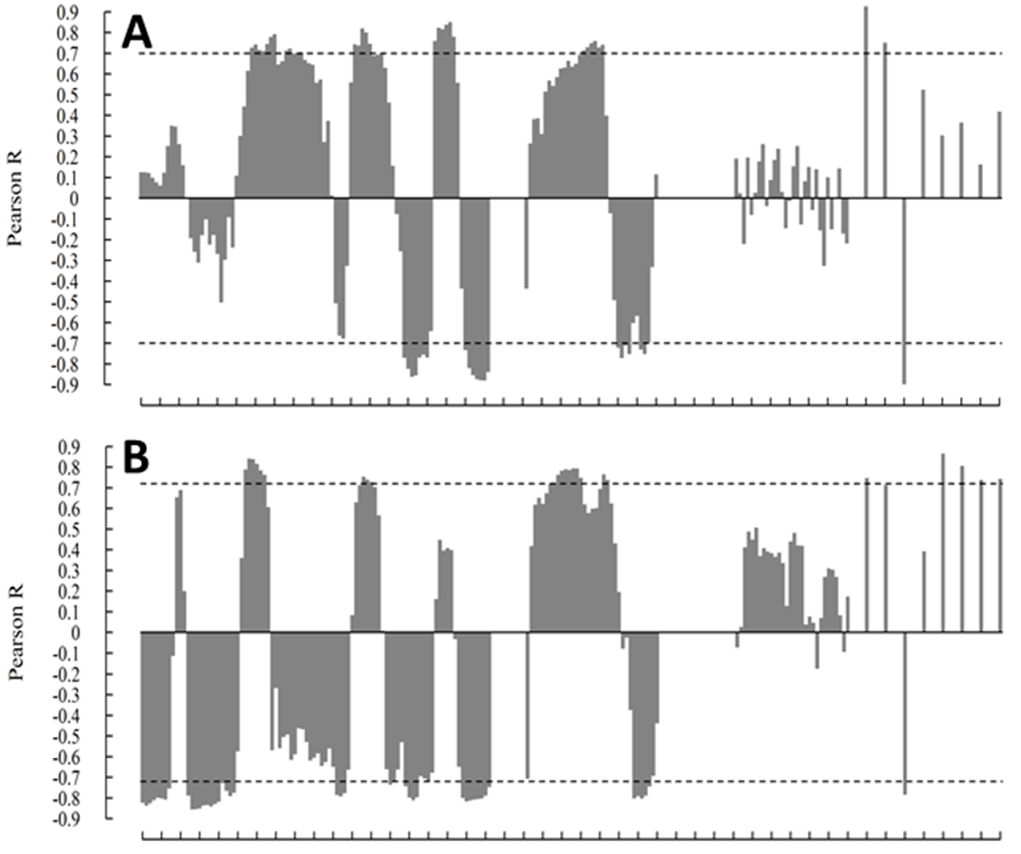
3.3.1. MBVI
| Rice | X | m | b | R2 | ΔR2 | p | Alfalfa | X | m | b | R2 | ΔR2 | p |
|---|---|---|---|---|---|---|---|---|---|---|---|---|---|
| 1 | Height | 0.05 | 7.78 | 0.85 | *** | 1 | EXGR | 7.00 | 8.34 | 0.75 | *** | ||
| 2 | Height | 0.03 | 7.64 | 0.88 | 0.03 | *** | 2 | EXGR | 4.73 | 10.32 | 0.78 | 0.04 | *** |
| λ1003 | 2.37 | *** | λ428' | −4257.59 | *** | ||||||||
| 3 | Height | 0.04 | 7.58 | 0.89 | 0.01 | *** | 3 | EXGR | 5.42 | 10.44 | 0.81 | 0.03 | *** |
| λ963 | −42.96 | ** | λ438' | −14925.85 | *** | ||||||||
| λ993 | 45.05 | ** | λ478' | 12192.62 | *** | ||||||||
| 4 | Height | 0.03 | 7.98 | 0.90 | 0.01 | *** | 4 | meanG | 22.14 | 4.81 | 0.82 | 0.01 | *** |
| λ1165 | −18.56 | ** | λ631' | −5177.17 | ** | ||||||||
| λ1003 | 54.20 | *** | λ468' | 15,276.97 | *** | ||||||||
| λ943 | −34.59 | *** | λ438' | −16,395.74 | *** | ||||||||
| 5 | Height | 0.04 | 7.68 | 0.91 | 0.00 | *** | 5 | meanG | 15.56 | 6.19 | 0.83 | 0.01 | *** |
| λ855 | 200.50 | *** | λ631' | −13,701.27 | *** | ||||||||
| λ824 | −956.69 | *** | λ621' | 26,155.46 | *** | ||||||||
| λ814 | 829.14 | ** | λ580' | −8975.98 | *** | ||||||||
| λ783 | −70.91 | ** | λ438' | −9906.12 | *** | ||||||||
| Cotton | X | m | b | R2 | ΔR2 | p | Maize | X | m | b | R2 | ΔR2 | p |
| 1 | Β | −6.16 | 13.56 | 0.83 | *** | 1 | Height | 0.01 | 11.74 | 0.63 | *** | ||
| 2 | Height | 0.04 | 9.90 | 0.87 | 0.04 | *** | 2 | Height | 0.00 | 12.46 | 0.68 | 0.05 | *** |
| λ672 | −17.13 | *** | β | −1.60 | *** | ||||||||
| 3 | Height | 0.03 | 8.81 | 0.88 | 0.01 | *** | 3 | Height | 0.00 | 11.32 | 0.69 | 0.01 | *** |
| λ1134 | 5.88 | *** | LAI | 0.09 | *** | ||||||||
| λ539 | −25.70 | *** | λ743 | 0.98 | ** | ||||||||
| 4 | Height | 0.02 | 8.93 | 0.90 | 0.01 | *** | 4 | Height | 0.01 | 11.41 | 0.71 | 0.02 | *** |
| λ1124 | 43.31 | *** | LAI | 0.10 | *** | ||||||||
| λ953 | −40.81 | *** | λ1114 | −12.30 | ** | ||||||||
| λ672 | −21.77 | *** | λ963 | 13.39 | ** | ||||||||
| 5 | Height | 0.03 | 8.73 | 0.90 | 0.01 | *** | 5 | Height | 0.00 | 12.56 | 0.74 | 0.03 | *** |
| λ1134 | 4.73 | *** | β | −1.70 | *** | ||||||||
| λ702 | −85.48 | *** | λ865 | −422.65 | *** | ||||||||
| λ692 | 361.94 | *** | λ845 | 560.70 | *** | ||||||||
| λ682 | −298.51 | *** | λ794 | −137.58 | *** |
3.3.2. TBVI
| Rice | X | M | b | R2 | ΔR2 | p | Alfalfa | X | m | b | R2 | ΔR2 | p |
|---|---|---|---|---|---|---|---|---|---|---|---|---|---|
| 1 | H | 0.05 | 7.78 | 0.85 | *** | 1 | λ1588', λ438' | −5.99 | 8.03 | 0.78 | *** | ||
| 2 | H | 0.03 | 7.84 | 0.88 | 0.04 | *** | 2 | λ1588', λ428' | −4.74 | 2.89 | 0.83 | 0.04 | *** |
| λ1266, λ1165 | −42.08 | *** | meanG | 15.84 | *** | ||||||||
| 3 | H | 0.03 | 8.25 | 0.89 | 0.01 | *** | 3 | λ1588', λ428' | −5.38 | 0.85 | 0.02 | *** | |
| λ993, λ753 | −2.68 | *** | meanG | 49.29 | *** | ||||||||
| λ1256, λ1235 | −73.92 | ** | medianG | −39.41 | *** | ||||||||
| 4 | λ1588', λ428' | −3.96 | 9.30 | 0.86 | 0.01 | *** | |||||||
| meanG | 49.84 | *** | |||||||||||
| medianG | −48.77 | *** | |||||||||||
| λ499', λ458' | −2.72 | ** | |||||||||||
| 5 | λ1528', λ438' | −16.82 | 9.24 | 0.89 | 0.02 | *** | |||||||
| meanG | 46.66 | *** | |||||||||||
| medianG | −44.81 | *** | |||||||||||
| λ499', λ458' | −4.46 | *** | |||||||||||
| λ1508', λ448' | 14.98 | *** | |||||||||||
| Cotton | X | M | b | R2 | ΔR2 | p | Maize | X | m | b | R2 | ΔR2 | p |
| 1 | λ1124, λ550 | −15.09 | 1.07 | 0.83 | *** | 1 | H | 0.01 | 11.65 | 0.63 | *** | ||
| 2 | λ1124, λ539 | −9.33 | 2.96 | 0.90 | 0.07 | *** | 2 | H | 0.00 | 12.42 | 0.68 | 0.05 | *** |
| H | 0.03 | *** | β | −1.72 | *** | ||||||||
| 3 | λ943, λ539 | −78.35 | −0.57 | 0.90 | 0.01 | *** | 3 | λ1034, λ428 | 68.14 | 13.99 | 0.70 | 0.01 | *** |
| λ963, λ560 | 66.64 | *** | λ933, λ428 | −65.48 | *** | ||||||||
| H | 0.03 | *** | H | 0.01 | *** | ||||||||
| 4 | λ973, λ550 | −130.15 | 0.81 | 0.91 | 0.01 | *** | 4 | λ1003, λ428 | 258.21 | 14.41 | 0.72 | 0.02 | *** |
| λ1104, λ570 | −60.57 | *** | λ983, λ428 | −255.45 | *** | ||||||||
| λ993, λ560 | 180.11 | *** | H | 0.01 | *** | ||||||||
| H | 0.02 | *** | LAI | 0.08 | *** | ||||||||
| 5 | λ943, λ539 | −243.81 | 1.03 | 0.91 | 0.01 | *** | 5 | λ1003, λ428 | 233.33 | 14.84 | 0.73 | 0.01 | *** |
| λ953, λ560 | 235.36 | *** | λ983, λ428 | −251.92 | *** | ||||||||
| λ1104, λ570 | −106.05 | *** | λ1155, λ428 | 22.15 | *** | ||||||||
| λ1064, λ529 | 105.00 | *** | H | 0.01 | *** | ||||||||
| H | 0.02 | *** | LAI | 0.08 | *** |
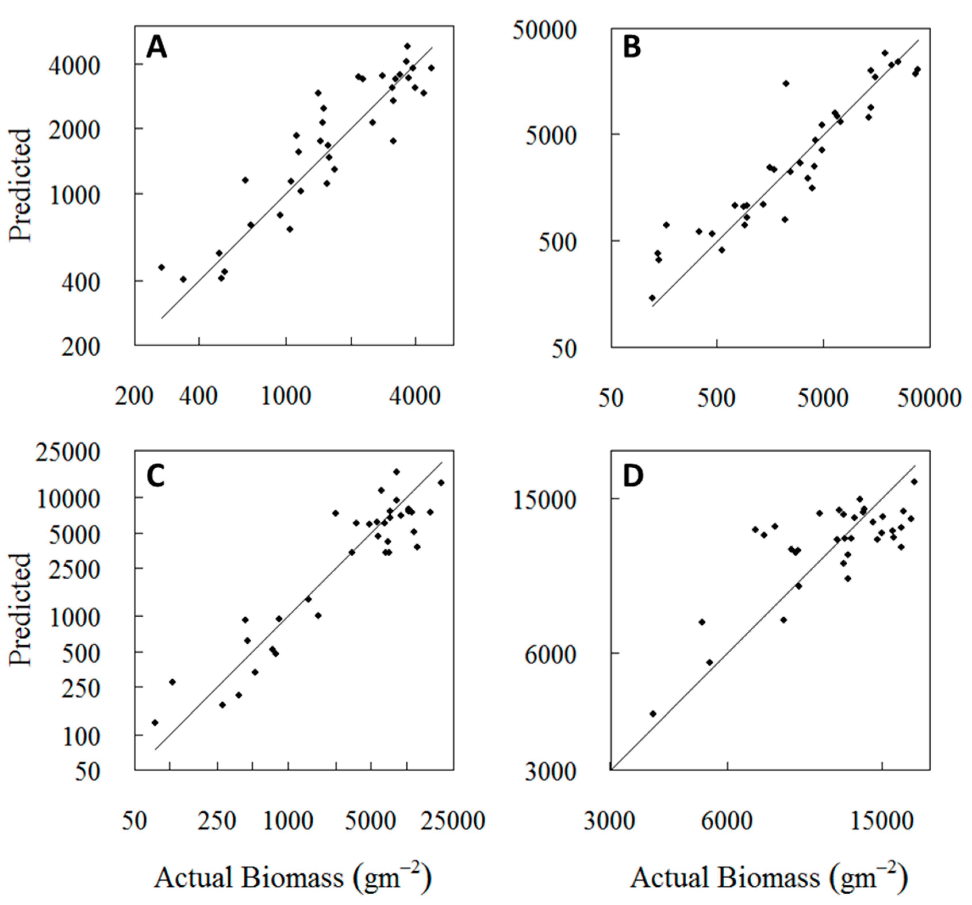
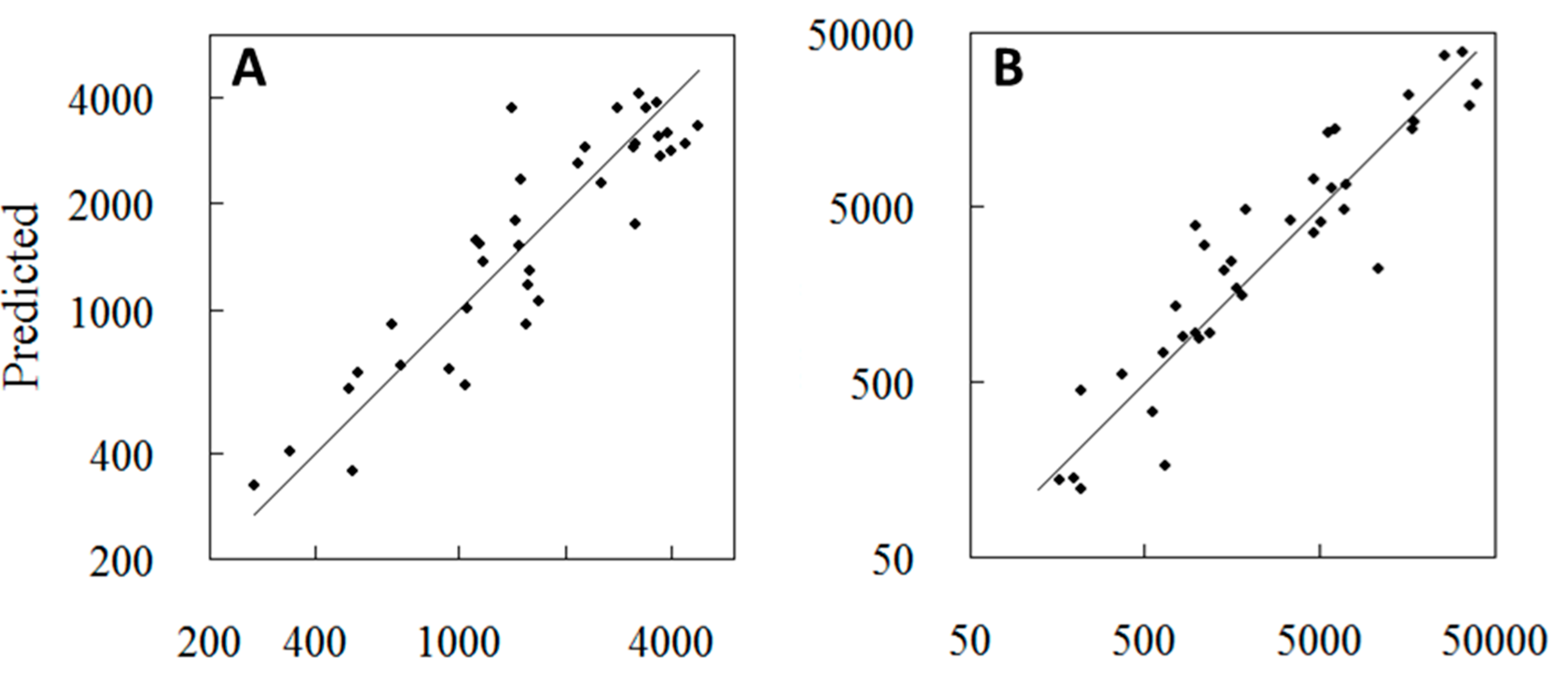
3.4. Model Validation


4. Discussion
5. Conclusions
Acknowledgments
Author Contributions
Conflicts of Interest
References
- Houghton, R.A. Aboveground forest biomass and the global carbon balance. Glob. Chang. Biol. 2005, 11, 945–958. [Google Scholar] [CrossRef]
- IPCC. Climate Change 2013: The Physical Science Basis. Contribution of Working Group I to the Fifth Assessment Report of the Intergovernmental Panel on Climate Change; Cambridge University Press: Cambridge, UK, 2013; p. 1535. [Google Scholar]
- Valentini, R.; Arneth, A.; Bombelli, A.; Castaldi, S.; Cazzolla Gatti, R.; Chevallier, F.; Ciais, P.; Grieco, E.; Hartmann, J.; Henry, M.; et al. A full greenhouse gases budget of Africa: Synthesis, uncertainties, and vulnerabilities. Biogeosciences 2014, 11, 381–407. [Google Scholar] [CrossRef]
- Schoeneberger, M.; Bentrup, G.; Gooijer, H.; de Soolanayakanahally, R.; Sauer, T.; Brandle, J.; Zhou, X.; Current, D. Branching out: Agroforestry as a climate change mitigation and adaptation tool for agriculture. J. Soil Water Conserv. 2012, 67, 128A–136A. [Google Scholar] [CrossRef]
- Sellers, P.J. Canopy reflectance, photosynthesis and transpiration. Int. J. Remote Sens. 1985, 6, 1335–1372. [Google Scholar] [CrossRef]
- Challinor, A.J.; Ewert, F.; Arnold, S.; Simelton, E.; Fraser, E. Crops and climate change: Progress, trends, and challenges in simulating impacts and informing adaptation. J. Exp. Bot. 2009, 60, 2775–2789. [Google Scholar] [CrossRef] [PubMed]
- Hay, R.K.M. Harvest index: A review of its use in plant breeding and crop physiology. Ann. Appl. Biol. 1995, 126, 197–216. [Google Scholar] [CrossRef]
- Prince, S.D.; Haskett, J.; Steininger, M.; Strand, H.; Wright, R. Net primary production of U.S. midwest croplands from agricultural harvest yield data. Ecol. Appl. 2001, 11, 1194–1205. [Google Scholar] [CrossRef]
- Doraiswamy, P.C.; Moulin, S.; Cook, P.W.; Stern, A. Crop yield assessment from remote sensing. Photogramm. Eng. Remote Sens. 2003, 69, 665–674. [Google Scholar] [CrossRef]
- Lu, D. The potential and challenge of remote sensing-based biomass estimation. Int. J. Remote Sens. 2006, 27, 1297–1328. [Google Scholar] [CrossRef]
- Tucker, C.J. A critical review of remote sensing and other methods for non-destructive estimation of standing crop biomass. Grass Forage Sci. 1980, 35, 177–182. [Google Scholar] [CrossRef]
- Phinn, S.; Roelfsema, C.; Dekker, A.; Brando, V.; Anstee, J. Mapping seagrass species, cover and biomass in shallow waters: An assessment of satellite multi-spectral and airborne hyper-spectral imaging systems in Moreton Bay (Australia). Remote Sens. Environ. 2008, 112, 3413–3425. [Google Scholar] [CrossRef]
- Catchpole, W.R.; Wheeler, C.J. Estimating plant biomass: A review of techniques. Aust. J. Ecol. 1992, 17, 121–131. [Google Scholar] [CrossRef]
- Ganguli, A.C.; Vermeire, L.T.; Mitchell, R.B.; Wallace, M.C. Comparison of four nondestructive techniques for estimating standing crop in shortgrass plains. Agron. J. 2000, 92, 1211–1215. [Google Scholar] [CrossRef]
- Martin, R.C.; Astatkie, T.; Cooper, J.M.; Fredeen, A.H. A Comparison of methods used to determine biomass on naturalized swards. J. Agron. Crop Sci. 2005, 191, 152–160. [Google Scholar] [CrossRef]
- Flombaum, P.; Sala, O.E. A non-destructive and rapid method to estimate biomass and aboveground net primary production in arid environments. J. Arid Environ. 2007, 69, 352–358. [Google Scholar] [CrossRef]
- Hutchings, N.J. Spatial heterogeneity and other sources of variance in sward height as measured by the sonic and HFRO sward sticks. Grass Forage Sci. 1991, 46, 277–282. [Google Scholar] [CrossRef]
- Paruelo, J.M.; Lauenroth, W.K.; Roset, P.A. Estimating aboveground plant biomass using a photographic technique. J. Range Manag. 2000, 53, 190–193. [Google Scholar] [CrossRef]
- Serrano, J.M.; Peça, J.O.; da Silva, J.M.; Shahidian, S. Calibration of a capacitance probe for measurement and mapping of dry matter yield in Mediterranean pastures. Precis. Agric. 2011, 12, 860–875. [Google Scholar] [CrossRef]
- Gourley, C.; McGowan, A. Assessing differences in pasture mass with an automated rising plate meter and a direct harvesting technique. Aust. J. Exp. Agric. 1991, 31, 337–339. [Google Scholar] [CrossRef]
- Ehlert, D.; Hammen, V.; Adamek, R. On-line sensor pendulum-meter for determination of plant mass. Precis. Agric. 2003, 4, 139–148. [Google Scholar] [CrossRef]
- Ollinger, S.V. Sources of variability in canopy reflectance and the convergent properties of plants. New Phytol. 2011, 189, 375–394. [Google Scholar] [CrossRef] [PubMed]
- Pinter, P.J.; Hatfield, J.L.; Schepers, J.S.; Barnes, E.M.; Moran, M.S.; Daughtry, C.S.T.; Upchurch, D.R. Remote sensing for crop management. Photogramm. Eng. Remote Sens. 2003, 69, 647–664. [Google Scholar] [CrossRef]
- Horler, D.N.H.; Dockray, M.; Barber, J. The red edge of plant leaf reflectance. Int. J. Remote Sens. 1983, 4, 273–288. [Google Scholar] [CrossRef]
- Perry, E.M.; Roberts, D.A. Sensitivity of narrow-band and broad-band indices for assessing nitrogen availability and water stress in an annual crop. Agron. J. 2008, 100, 1211–1219. [Google Scholar] [CrossRef]
- Ustin, S.L.; Roberts, D.A.; Gamon, J.A.; Asner, G.P.; Green, R.O. Using imaging spectroscopy to study ecosystem processes and properties. BioScience 2004, 54, 523–533. [Google Scholar] [CrossRef]
- Goetz, A.F.H. Three decades of hyperspectral remote sensing of the earth: A personal view. Remote Sens. Environ. 2009, 113, S5–S16. [Google Scholar] [CrossRef]
- Carter, G.A. Primary and secondary effects of water content of the spectral reflectance of leaves. Am. J. Bot. 1991, 78, 916–924. [Google Scholar] [CrossRef]
- Asner, G.P. Biophysical and biochemical sources of variability in canopy reflectance. Remote Sens. Environ. 1998, 64, 234–253. [Google Scholar] [CrossRef]
- HyspIRI Mission Study. Available online: http://hyspiri.jpl.nasa.gov/ (accessed on 3 December 2014).
- Thenkabail, P.S.; Ward, A.D.; Lyon, J.G. Landsat-5 thematic mapper models of soybean and corn crop characteristics. Int. J. Remote Sens. 1994, 15, 49–61. [Google Scholar] [CrossRef]
- Thenkabail, P.S.; Ward, A.D.; Lyon, J.G.; Merry, C.J. Thematic mapper vegetation indices for determining soybean and corn growth parameters. Photogramm. Eng. Remote Sens. 1994, 60, 437–442. [Google Scholar]
- Thenkabail, P.S.; Smith, R.B.; de Pauw, E. Hyperspectral vegetation indices and their Relationships with agricultural crop characteristics. Remote Sens. Environ. 2000, 71, 158–182. [Google Scholar] [CrossRef]
- Thenkabail, P.S.; Enclona, E.A.; Ashton, M.S.; Legg, C.; de Dieu, M.J. Hyperion, IKONOS, ALI, and ETM+ sensors in the study of African rainforests. Remote Sens. Environ. 2004, 90, 23–43. [Google Scholar] [CrossRef]
- CDFA. California Agricultural Statistics Review 2012–2013; California Department of Food and Agriculture: Sacramento, CA, USA, 2013; p. 131. [Google Scholar]
- USDA. 2007 Census of Agriculture; United States Department of Agriculture: Washington, DC, USA, 2009; p. 739. [Google Scholar]
- Faunt, C.C. Groundwater Availability of the Central Valley Aquifer; U.S. Geological Survey Professional Paper No. 1766; United State Geological Survey: Sacramento, CA, USA, 2009; p. 225. [Google Scholar]
- California Department of Water Resources. Available online: http://www.water.ca.gov/ (accessed on 3 December 2014).
- California Water Science Center. Available online: http://ca.water.usgs.gov/ (accessed on 3 December 2014).
- USDA CropScape. Available online: http://nassgeodata.gmu.edu/CropScape/ (accessed on 3 December 2014).
- McCoy, R.M. Field Methods in Remote Sensing; The Guilford Press: New York, NY, USA, 2005. [Google Scholar]
- Liu, J.; Pattey, E. Retrieval of leaf area index from top-of-canopy digital photography over agricultural crops. Agric. For. Meteorol. 2010, 150, 1485–1490. [Google Scholar] [CrossRef]
- Pérez, A.J.; López, F.; Benlloch, J.V.; Christensen, S. Colour and shape analysis techniques for weed detection in cereal fields. Comput. Electron. Agric. 2000, 25, 197–212. [Google Scholar] [CrossRef]
- Woebbecke, D.M.; Meyer, G.E.; von Bargen, K.; Mortensen, D.A. Color indices for weed identification under various soil, residue, and lighting conditions. Trans. ASAE 1995, 38, 259–269. [Google Scholar] [CrossRef]
- Meyer, G.E.; Neto, J.C. Verification of color vegetation indices for automated crop imaging applications. Comput. Electron. Agric. 2008, 63, 282–293. [Google Scholar] [CrossRef]
- Otsu, N. A threshold selection method from gray-level histograms. Automatica 1975, 11, 23–27. [Google Scholar]
- Meyer, G.E.; Hindman, T.W.; Laksmi, K. Machine vision detection parameters for plant species identification. Proc. SPIE 1999, 3543. [Google Scholar] [CrossRef]
- Sonnentag, O.; Hufkens, K.; Teshera-Sterne, C.; Young, A.M.; Friedl, M.; Braswell, B.H.; Richardson, A.D. Digital repeat photography for phenological research in forest ecosystems. Agric. For. Meteorol. 2012, 152, 159–177. [Google Scholar] [CrossRef]
- Decagon Devices, Inc. Available online: http://www.decagon.com/ (accessed 3 December 2014).
- Wilhelm, W.W.; Ruwe, K.; Schlemmer, M.R. Comparison of three leaf area index meters in a corn canopy. Crop Sci. 2000, 40, 1179–1183. [Google Scholar] [CrossRef]
- Decagon. In AccuPAR PAR/LAI Ceptometer Model LP-80; Version 10; Decagon Devices, Inc.: Pullman, WA, USA, 2010.
- ASD Inc. Available online: http://www.asdi.com/ (accessed 3 December 2014).
- Marshall, M.; Thenkabail, P. Biomass modeling of four leading world crops using hyperspectral narrowbands in support of HyspIRI mission. Photogramm. Eng. Remote Sens. 2014, 80, 757–772. [Google Scholar] [CrossRef]
- MacArthur, A.; MacLellan, C.J.; Malthus, T. The fields of view and directional response functions of two field spectroradiometers. IEEE Trans. Geosci. Remote Sens. 2012, 50, 3892–3907. [Google Scholar] [CrossRef]
- The Comprehensive R Archive Network. Available online: http://cran.r-project.org/ (accessed 3 December 2014).
- Serrano, L.; Peñuelas, J.; Ustin, S.L. Remote sensing of nitrogen and lignin in Mediterranean vegetation from AVIRIS data: Decomposing biochemical from structural signals. Remote Sens. Environ. 2002, 81, 355–364. [Google Scholar] [CrossRef]
- Thorp, K.R.; Tian, L.; Yao, H.; Tang, L. Narrow-Band and derivative-based vegetation indices for hyperspectral data. Trans. ASAE 2004, 47, 291–299. [Google Scholar] [CrossRef]
- Hair, J.F., Jr.; Anderson, R.E.; Tatham, R.L.; Black, W.C. Multivariate Data Analysis, 5th ed.; Prentice Hall: Upper Saddle River, NJ, USA, 1998. [Google Scholar]
- Tucker, C.J. Red and photographic infrared linear combinations for monitoring vegetation. Remote Sens. Environ. 1979, 8, 127–150. [Google Scholar] [CrossRef]
- Skye Instruments. Available online: http://www.skyeinstruments.com/ (accessed on 3 December 2014).
- Mariotto, I.; Thenkabail, P.S.; Huete, H.; Slonecker, T.; Platonov, A. Hyperspectral versus multispectral crop- biophysical modeling and type discrimination for the HyspIRI mission. Remote Sens. Environ. 2013, 139, 291–305. [Google Scholar] [CrossRef]
- Gnyp, M.L.; Miao, Y.; Yuan, F.; Ustin, S.L.; Yu, K.; Yao, Y.; Bareth, G. Hyperspectral canopy sensing of paddy rice aboveground biomass at different growth stages. Field Crops Res. 2014, 155, 42–55. [Google Scholar] [CrossRef]
- Atzberger, C.; Guérif, M.; Baret, F.; Werner, W. Comparative analysis of three chemometric techniques for the spectroradiometric assessment of canopy chlorophyll content in winter wheat. Comput. Electron. Agric. 2010, 73, 165–173. [Google Scholar] [CrossRef]
- Moran, M.S.; Pinter, P.J., Jr.; Clothier, B.E.; Allen, S.G. Effect of water stress on the canopy architecture and spectral indices of irrigated Alfalfa. Remote Sens. Environ. 1989, 29, 251–261. [Google Scholar] [CrossRef]
- Bai, J.; LI, S.; Wang, K.; SUI, X.; Chen, B.; Wang, F. Estimating aboveground fresh biomass of different cotton canopy types with homogeneity models based on hyper spectrum parameters. Agric. Sci. China 2007, 6, 437–445. [Google Scholar] [CrossRef]
- Jacquemoud, S.; Verhoef, W.; Baret, F.; Bacour, C.; Zarco-Tejada, P.J.; Asner, G.P.; Francois, C.; Ustin, S.L. PROSPECT + SAIL models: A review of use for vegetation characterization. Remote Sens. Environ. 2009, 113, S56–S66. [Google Scholar] [CrossRef]
- Lim, K.; Treitz, P.; Wulder, M.; St-Onge, B.; Flood, M. LiDAR remote sensing of forest structure. Prog. Phys. Geogr. 2003, 27, 88–106. [Google Scholar] [CrossRef]
- Thenkabail, P.S.; Mariotto, I.; Gumma, M.K.; Middleton, E.M.; Landis, D.R.; Huemmrich, K.F. Selection of Hyperspectral Narrowbands (HNBs) and composition of Hyperspectral two band Vegetation Indices (HVIs) for biophysical characterization and discrimination of crop types using field reflectance and hyperion/EO-1 data. IEEE J. Sel. Top. Appl. Earth Obs. Remote Sens. 2013, 6, 427–439. [Google Scholar] [CrossRef]
- Tsai, F.; Philpot, W. Derivative analysis of hyperspectral data. Remote Sens. 1998, 66, 41–51. [Google Scholar] [CrossRef]
- Huang, Z.; Turner, B.J.; Dury, S.J.; Wallis, I.R.; Foley, W.J. Estimating foliage nitrogen concentration from HYMAP data using continuum removal analysis. Remote Sens. Environ. 2004, 93, 18–29. [Google Scholar] [CrossRef]
- Combal, B.; Baret, F.; Weiss, M.; Trubuil, A.; Macé, D.; Pragnère, A.; Myeni, R.; Wang, L. Retrieval of canopy biophysical variables from bidirectional reflectance: Using prior information to solve the ill-posed inverse problem. Remote Sens. Environ. 2003, 84, 1–15. [Google Scholar] [CrossRef]
© 2015 by the authors; licensee MDPI, Basel, Switzerland. This article is an open access article distributed under the terms and conditions of the Creative Commons Attribution license (http://creativecommons.org/licenses/by/4.0/).
Share and Cite
Marshall, M.; Thenkabail, P. Developing in situ Non-Destructive Estimates of Crop Biomass to Address Issues of Scale in Remote Sensing. Remote Sens. 2015, 7, 808-835. https://doi.org/10.3390/rs70100808
Marshall M, Thenkabail P. Developing in situ Non-Destructive Estimates of Crop Biomass to Address Issues of Scale in Remote Sensing. Remote Sensing. 2015; 7(1):808-835. https://doi.org/10.3390/rs70100808
Chicago/Turabian StyleMarshall, Michael, and Prasad Thenkabail. 2015. "Developing in situ Non-Destructive Estimates of Crop Biomass to Address Issues of Scale in Remote Sensing" Remote Sensing 7, no. 1: 808-835. https://doi.org/10.3390/rs70100808
APA StyleMarshall, M., & Thenkabail, P. (2015). Developing in situ Non-Destructive Estimates of Crop Biomass to Address Issues of Scale in Remote Sensing. Remote Sensing, 7(1), 808-835. https://doi.org/10.3390/rs70100808