PSI Deformation Map Retrieval by Means of Temporal Sublook Coherence on Reduced Sets of SAR Images

Abstract

Prior to the application of any persistent scatterer interferometry (PSI) technique for the monitoring of terrain displacement phenomena, an adequate pixel selection must be carried out in order to prevent the inclusion of noisy pixels in the processing. The rationale is to detect the so-called persistent scatterers, which are characterized by preserving their phase quality along the multi-temporal set of synthetic aperture radar (SAR) images available. Two criteria are mainly available for the estimation of pixels’ phase quality, i.e., the coherence stability and the amplitude dispersion or permanent scatterers (PS) approach. The coherence stability method allows an accurate estimation of the phase statistics, even when a reduced number of SAR acquisitions is available. Unfortunately, it requires the multi-looking of data during the coherence estimation, leading to a spatial resolution loss in the final results. In contrast, the PS approach works at full-resolution, but it demands a larger number of SAR images to be reliable, typically more than 20. There is hence a clear limitation when a full-resolution PSI processing is to be carried out and the number of acquisitions available is small. In this context, a novel pixel selection method based on exploiting the spectral properties of point-like scatterers, referred to as temporal sublook coherence (TSC), has been recently proposed. This paper seeks to demonstrate the advantages of employing PSI techniques by means of TSC on both orbital and ground-based SAR (GB-SAR) data when the number of images available is small (10 images in the work presented). The displacement maps retrieved through the proposed technique are compared, in terms of pixel density and phase quality, with traditional criteria. Two X-band datasets composed of 10 sliding spotlight TerraSAR-X images and 10 GB-SAR images, respectively, over the landslide of El Forn de Canillo (Andorran Pyrenees), are employed for this study. For both datasets, the TSC technique has showed an excellent performance compared with traditional techniques, achieving up to a four-fold increase in the number of persistent scatters detected, compared with the coherence stability approach, and a similar density compared with the PS approach, but free of outliers.

1. Introduction

Data acquired from synthetic aperture radar (SAR) sensors allows obtaining all-day, all-weather high-resolution complex reflectivity images of large-scale areas. If SAR images are taken at different times, differential SAR interferometry (DInSAR) techniques allow exploiting phase differences, i.e., the interferograms, between multi-temporal pairs of single look complex (SLC) images in order to retrieve the displacement information of affected areas [1,2] with millimetric precision [3]. The exploitation of the interferometric phase is limited by geometrical and temporal decorrelation phenomena [4]. The presence of hard atmospheric artifacts also compromises the applicability of classical DInSAR techniques.

In order to overcome these limitations, different persistent scatterer interferometry (PSI) techniques have been developed during the last decade [5,6,7,8,9,10,11,12,13,14,15]. In this case, large datasets of multi-temporal SAR data are employed in order to generate multiple phase relationships, allowing the reliable estimation of both the linear and the non-linear component of terrain displacements, as well as the atmospheric phase screen (APS) for each acquisition. Nowadays, there exist a lot of applications showing their validity for monitoring large-scale deformation episodes, as well as providing a useful technique for their geophysical interpretation. Examples of such applications include, among others, modeling surface deformation [16,17,18], glacier monitoring [19], landslides [20], soil compaction rate [21] or atmosphere estimation [4].

As happened with classical DInSAR, the achievable velocity map reliability also depends on the pixels affected by decorrelation phenomena. The displacement information cannot thus be exploited from all pixels within the illuminated scenario, as only a limited number of them, the so-called persistent scatterers, fulfill the phase quality requirements to be included in the PSI processing.

Two main criteria are available for the estimation of pixels’ phase quality: these are the coherence stability [12,18] and the permanent scatterer (PS) approach [6]. The former makes use of the estimated coherence maps from the multi-looked interferograms, which can be directly related with the standard deviation of the interferometric phase. The multi-look (ML) used, which basically consists of applying a boxcar window, reduces the resolution of the interferograms depending on the averaging factor employed. This fact impacts the pixel selection step, leading to an inherent reduction of the resolution during the detection of persistent scatterers. For this reason, this approach is typically addressed as low-resolution PSI. The latter relates the phase dispersion of those scatterers presenting high values of signal-to-noise ratio (SNR) with the amplitude dispersion (D_A) estimator [6], which basically corresponds to a measure of the pixels’ amplitude stability. Pixels stable in amplitude are assumed to be reliable in phase. Since the multi-looking of data is not required in that case, the resolution of the original images is preserved during the detection of persistent scatterers. For this reason, this method is typically addressed as full-resolution PSI.

The choice of the pixel selection criterion basically depends on the number of acquisitions at disposal, on the resolution required and on the nature of the scenario to be monitored. On the one hand, the coherence stability method ensures accurate estimations of the phase statistics, even when a reduced number of SAR images is available. In contrast, the PS approach demands a larger number of SAR images to be reliable, typically more than 20 [6]. On the other hand, the coherence stability criterion performs better over environments with the predominance of distributed targets; this is when multiple scatters are present within a resolution cell. In contrast, the PS approach is mainly employed for the detection of deterministic point-like targets, such as man-made structures, which are not affected by geometrical decorrelation and speckle noise, as there is a single dominant scatter within the resolution cell. There is hence a clear limitation when the full-resolution of SAR images requires being preserved to exploit the point-like scatters within the the illuminated scenario and the number of images available is small.

A clear example of this appears when SAR images of the so-called new family of X-band SAR sensors, like the German TerraSAR-X and TanDEM-X satellites [22,23] or the Italian constellation Cosmo-Skymed [24], are ordered for area monitoring. During the last few years, this new family of SAR sensors has led to a scientific breakthrough presenting low revisiting times (up to few days) and improved spatial resolutions (up to the meter), which are providing scientists outstanding amounts of unprecedented X-band SAR data. Nonetheless, the acquisition of these products has become considerably more expensive compared with its predecessors, such as ERS-1/2 or ENVISAT. This fact compromises in many cases the acquisition of a large number of SAR images with the lowest time lapses, since it considerably increases the cost of the monitoring and can make PSI techniques lose a competitive advantage against other surveying techniques. This is clearly the case of slow-moving phenomena monitoring, because large numbers of SAR images acquired in a short period of time do not provide new information. In addition, the high-resolution of the images, the shorter swaths and the multiple modes available make these data be acquired “under demand”. This implies that it will be very unlikely to have a historical archive of images of a particular area of interest. Finally, it must be pointed out that in the presence of large spatial baselines, understanding large as closer to the critical baseline, a big amount of coherence maps under the coherence stability approach cause some interferograms to be useless due to the geometrical decorrelation [6]. A full-resolution PSI processing is mandatory in all of these cases in order to benefit from the high-resolution provided by these sensors, even when a reduced set of SAR data is available.

Another interesting example arises from the use of ground-based SAR (GB-SAR) sensors when these are employed to carry out a discontinuous monitoring of affected areas. This operation mode consists of revisiting the area of interest during different measurement days at regular intervals, and it is typically addressed for the monitoring of slow-displacement rate phenomena, where performing a continuous monitoring is inefficient and costly. Once again, improving the performance of full-resolution PSI techniques when a reduced number of GB-SAR images is available is clearly interesting.

In order to overcome this limitation of classical PSI techniques, a new approach based on exploiting the spectral properties of point-like scatterers has been recently presented in [25]. This method takes advantage of the so-called coherent scatterers (CS), presented in [26], but including the temporal axis in the detection. The rationale is to estimate which targets exhibit a high spectral correlation coefficient along the multi-temporal set of SAR images available. This estimation is referred to as temporal sublook coherence (TSC). Those targets fulfilling this condition will be directly related to as point-like scatterers with reliable phases or following the nomenclature used in [25], as temporally stable coherent scatterers (SCS). To date, the application of PSI techniques by means of TSC has been demonstrated for urban subsidence monitoring using a large number of orbital SAR data. In that case, results have shown a similar performance if compared with the PS approach [25].

The objective of this paper is to demonstrate the applicability of the TSC approach for PSI purposes when a reduced number of SAR images is available. The estimation accuracy, the number of pixel candidates and the final PSI displacement maps retrieved are deeply discussed and compared with the classical approaches described above.

The test site selected to demonstrate the feasibility of the TSC approach corresponds to the slow-moving landslide of El Forn de Canillo, located in the Andorran Pyrenees. Applying PSI algorithms over this type of rural scenario, mostly vegetated, constitutes an extra challenge, in contrast with urban areas, where PSI techniques typically perform better. For this purpose, two datasets are employed. On the one hand, 10 sliding spotlight TerraSAR-X images covering the period from October 2010, to November 2011, are used. On the other hand, 10 X-band images collected during the same period with a frequency modulated continuous wave (FMCW) GB-SAR sensor are employed to complete the study. The inclinometric results available for the maximum displacement area of the landslide, known as Cal Boró-Cal Ponet, are used as ground-truth in order to validate the PSI results obtained.

The paper is structured as follows. Section 2 presents a description of the test site and the datasets employed for the study in order to introduce the reader to the context of this work. In Section 3, the sublook generation and TSC estimation processes are briefly reviewed. A comparison between the TSC and the traditional phase quality estimators is presented at this stage. Section 4 shows the relationship between the TSC metrics and the pixels’ phase dispersion. A comparison in terms of pixels selected between the TSC and the classical approaches is presented. Section 5 shows the final displacement maps retrieved by means of the TSC approach. These results are deeply discussed and compared with the ones obtained with the classical approaches. In addition, some ground-truth is shown in order to validate the displacement results retrieved. The main conclusions and major remarks of the manuscript are given in Section 6.

2. Test Site and Dataset

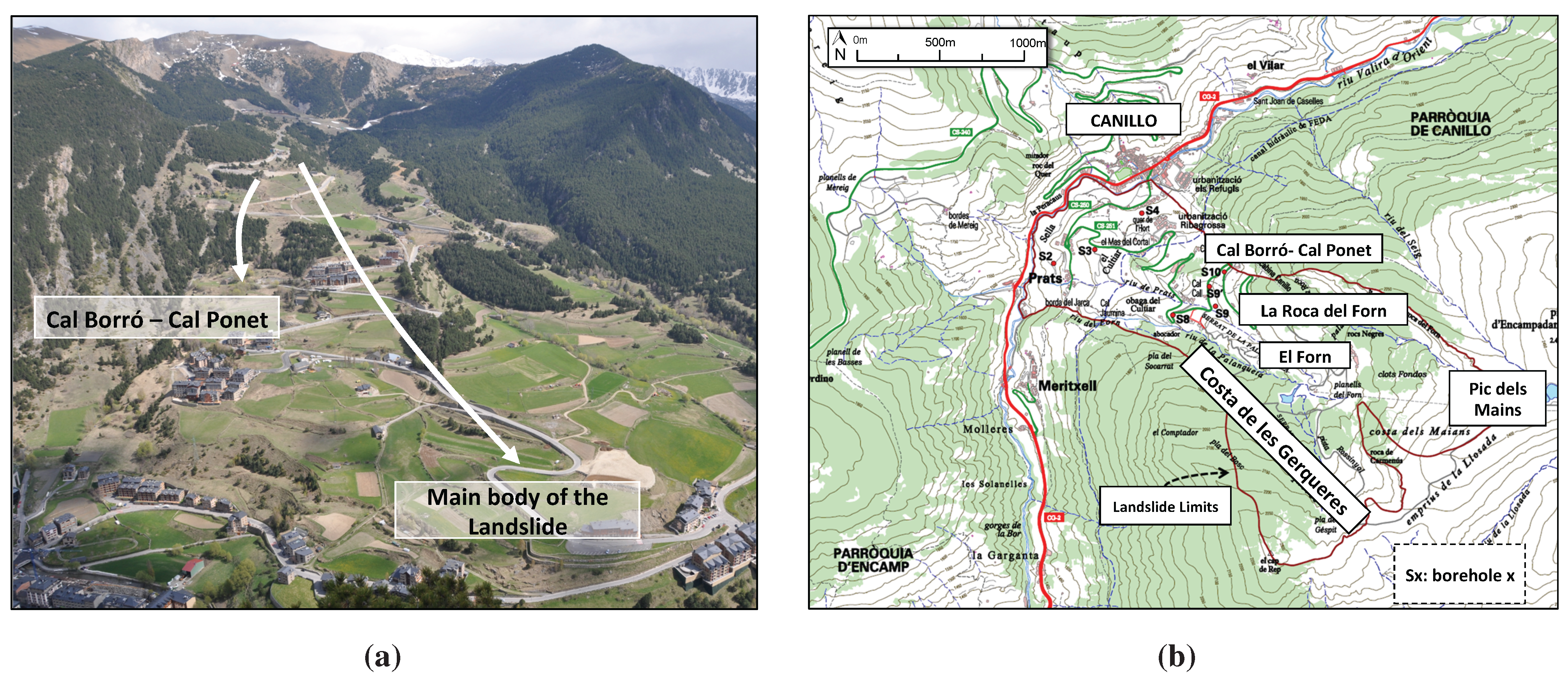
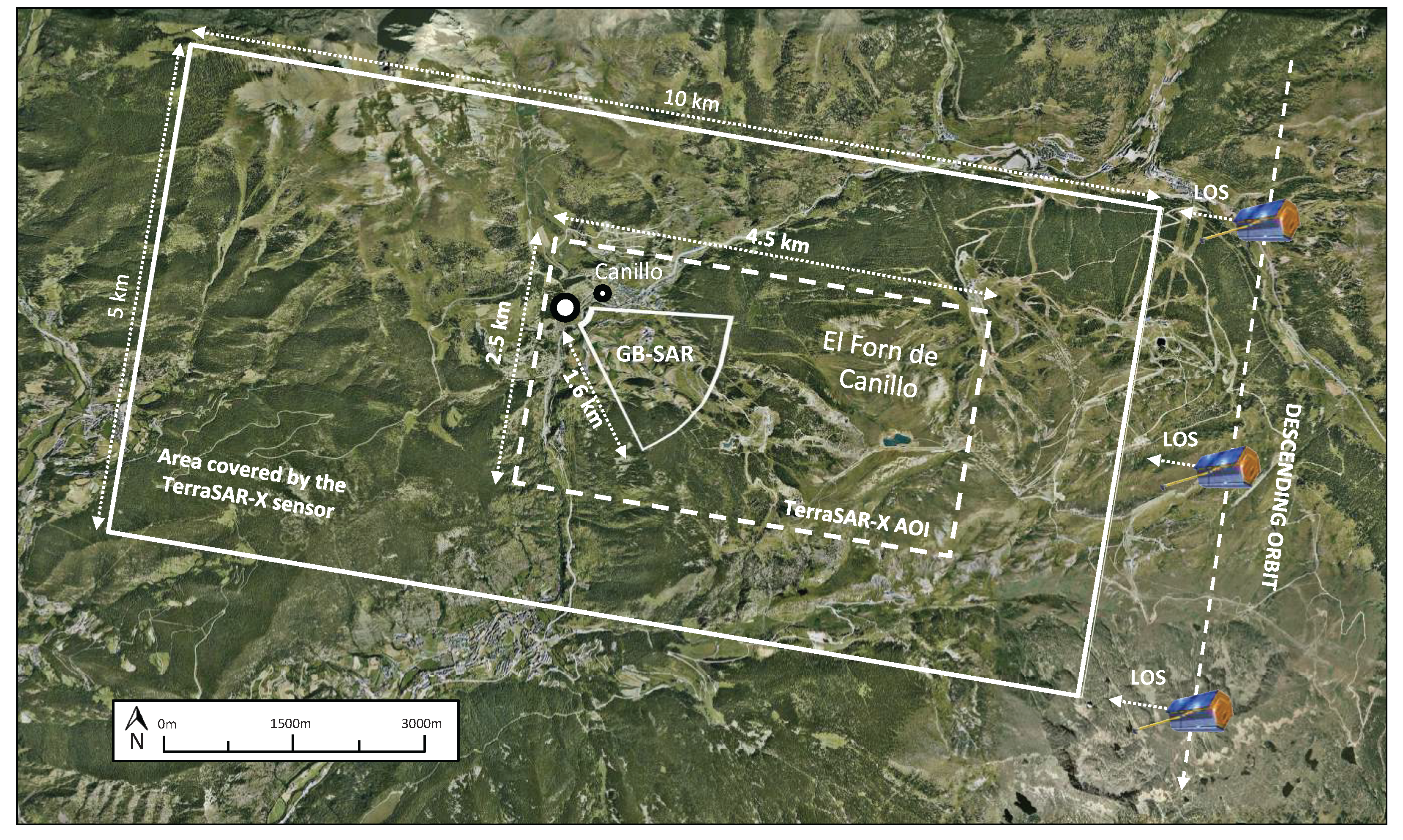
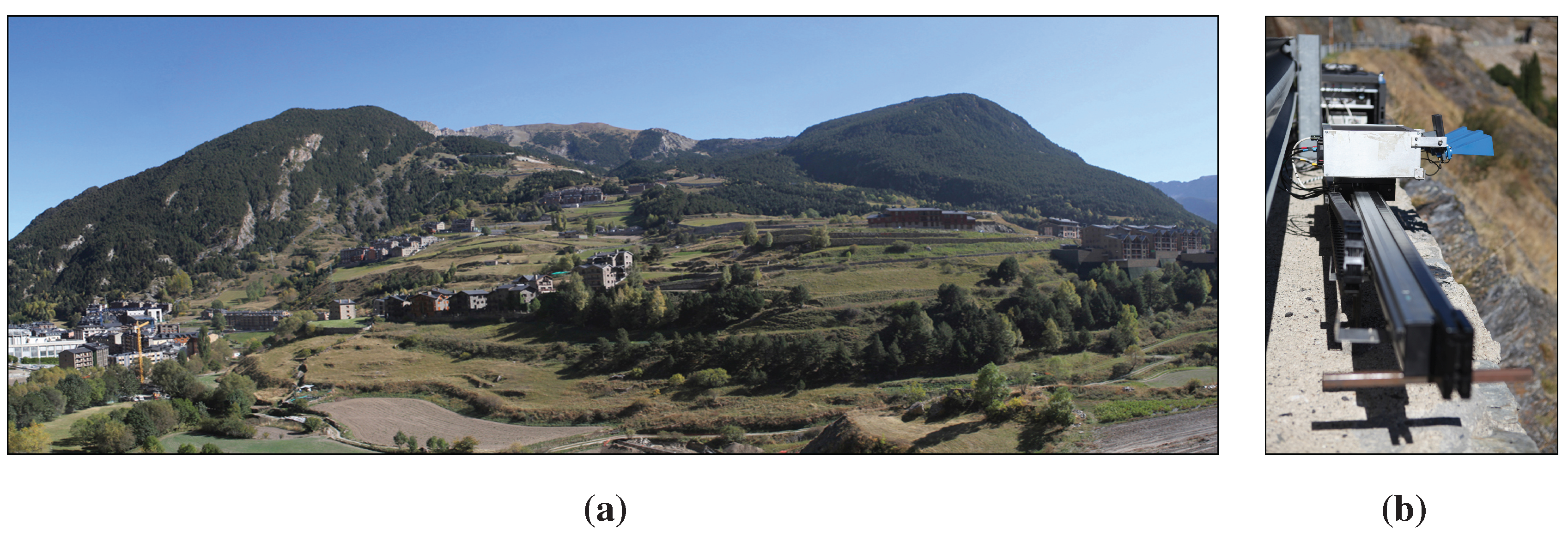
2.1. Test Site

The test site selected to evaluate the performance of the proposed technique corresponds to the area of El Forn de Canillo (located in the geographical coordinates 42.5610 north latitude and 1.6018 western longitude), which constitutes one of the biggest landslides of the Andorran Pyrenees; see Figure 1a.

Figure 1. (a) General overview of the landslide of El Forn de Canillo; (b) landslide limits and location of the in-field monitoring network installed (Points S2 to S10).

Figure 1. (a) General overview of the landslide of El Forn de Canillo; (b) landslide limits and location of the in-field monitoring network installed (Points S2 to S10).

The landslide is composed of a sequence of slides and earth-flows with a complex structure, which affects an estimated mass of around 300 Mm³. In this context, three major sliding units were identified in 1994 by Santacana [27]. The first one corresponds to a slide originated in the area of Pla del Géspit and Costa de les Gerqueres (see Figure 1b), located in the southwest of the landslide, which reached the foot of the hillside. A second unit originated under El Pic de Maians (see Figure 1b) reaching a height of 1640 m, and which overlaps with the previous sliding unit, closing in the Valira River valley. Finally, a new rotational slide with a lower extension originated on the hillside, known as La Roca del Forn (see Figure 1b), in the northeast side of the hillside, has been identified.

The landslide originated due to a decompression phenomenon after the removal of the Valira Glacier, between the years 13, 000 and 16, 000 BP [27]. Throughout the years, the Valira River has been progressively eroding the base of the whole hillside mass without reaching the bedrock, thus originating the landslide [27].

Different observations accumulated during the last few decades have evidenced that the slide mass is still active today, with a residual displacement of few centimeters per year. Concretely, a local failure in the area, known as Cal Borró-Cal Ponet, located in the northeast extreme of the main body of the landslide, has been recently identified, showing a higher activity coinciding with periods of intense rains and snow melting [28].

In the year 2000, the Andorran authorities promoted several actions for the management of the risk related with the geo-hazard threats associated with landslides, rockfalls and debris flows in the Andorran Pyrenees. Some specific management plans were carried out for the monitoring of El Forn de Canillo. Between the years 2007 and 2009, a network of geotechnical devices, including inclinometers, rod extensometers and piezometers, was installed over the surface of El Forn de Canillo to characterize and understand the dynamics of the landslide. A total of 10 boreholes, referred to as S2 to S10 in Figure 1b and reaching a depth between 40 and 60 m, were drilled and equipped with this instrumentation. The measurements provided by these devices have been recently studied with the objective of locating the sliding surfaces and characterizing the displaced material [28].

Unfortunately, some of the boreholes did not reach the needed depth, and consequently, the installed devices did not work properly in some points. Nonetheless, the measurements and observations carried out evidenced that, in addition to a residual movement of the landslide main lobe of some millimeters per year, the most active part corresponds to the secondary landslide of Cal Borró-Cal Ponet, which, between May and June, 2009, registered a velocity up to roughly 2 cm/month [28]. Intense sudden rain events and snow melting were observed during this period. Only those inclinometers reaching the needed depth continue working to date. This is the case of the one referred to as S10, located in the maximum displacement rate area of Cal Borró-Cal Ponet, which will be employed to validate the PSI results obtained in this work.

Finally, 3 GB-SAR campaigns carried out by the Institute of Geomatics (Spain) monitored a network composed of 15 corner reflectors over the area of Cal Borró-Cal Ponet. They covered a period of 57 days during fall, 2009, and registered displacements up to 14 mm [29]. This work concluded with the necessity of employing long-term remote sensing studies for the management of the risk related with the landslide of El Forn de Canillo.

2.2. Dataset

In light of all of this evidence, the use of both orbital and ground-based PSI techniques were planned in 2011. The reasons were two-fold. On the one hand, most of the geotechnical devices installed over the landslide surface did not work properly, providing unreliable measures, thus hindering the characterization of the landslide extension and dynamics. On the other hand, conventional geotechnical field measurements present lower densities and worse coverage compared with SAR techniques, which is a key factor in landslide characterization. In this framework, the remote sensing laboratory (RSLab), in collaboration with the Department of Geotechnical Engineering and Geosciences of the Universitat Politècnica de Catalunya (UPC), carried out a one-year monitoring work, from October 2010, to November 2011, employing SAR images acquired with the TerraSAR-X space-borne sensor in sliding spotlight mode and with the UPC’s GB-SAR system, referred to as RiskSAR-X. The RiskSAR-X sensor focused on the urbanized area of the landslide, located at the lower part of the sliding mass where the geotechnical devices were installed, while the sliding spotlight TerraSAR-X images covered the whole landslide extension.

Some important decisions, such as the orbit pass or the GB-SAR location, need to be further commented on at this point. These aspects are especially important in landslide monitoring applications that typically occur in steep topography scenarios, in which the acquisition geometry plays an important role. Minimizing the geometrical distortion effects of SAR imaging and maximizing the detection of the real ground displacement are key factors in order to improve the performance of PSI techniques. The former influences the area illuminated by the SAR sensor and, consequently, the quantity of useful information collected by it. The latter is related to the fact that SAR systems are only able to detect displacements in the line-of-sight (LOS) direction.

Three geometric distortions are present in SAR imaging regardless of the platform nature: the foreshortening, the layover and the shadowing [4]. For the current polar-orbiting SAR orbital sensors, the look direction is either east or west, for the ascending or descending pass, respectively. For this reason, SAR sensors only are able to detect movements along slopes facing either east or west and are almost insensitive to movements in the north or south directions. Since the landslide of El Forn de Canillo is facing west, the descending pass was finally selected to avoid foreshortening and layover phenomena in the illuminated area.

Moreover, it must be taken into account that SAR systems only have sensitivity to detect displacements in the LOS direction. For this reason, detected displacements are rarely the real ones, but a projection of them. In landslide applications, the more realistic assumption regarding the displacement direction consists of considering that it is produced along the steepest gradient of the slope. Again, the descending pass resulted in being more suited for this scenario, since the projection factor between the real displacement and the LOS directions was lower compared with the one provided by the ascending mode.

Unlike space-borne SAR sensors, which are constrained by the orbit pass, GB-SAR sensors allow fitting the sensor location and illumination angle to the specific characteristics of the area of interest. In order to minimize the foreshortening and to maximize the detection of the ground displacements considering that the slide moves along the steepest gradient of the terrain slope, the RiskSAR-X sensor was finally located at the foot of the landslide, 100 m away from the slope. Furthermore, this emplacement also minimized the shaded areas in the SAR images collected. In order to ensure a millimetric repositioning of the instrument to avoid a later co-registration of the data, the system was mounted over a cement base reinforced with a lightweight metallic frame. The RiskSAR-X system was placed on a base at approximately 30 centimeters above the ground to elevate the rail and reduce the impact of the nearby vegetation.

Figure 2 shows a Google Earth image indicating the TerraSAR-X coverage, the area of interest selected for the orbital PSI processing, the RiskSAR-X location and the area illuminated by the GB-SAR sensor. Figure 3a shows a panoramic view of El Forn de Canillo seen from the RiskSAR-X point of view, which is represented in Figure 3b.

Figure 2. Coverage of the TerraSAR-X and RiskSAR-X sensors over the area ofEl Forn de Canillo. The solid rectangle indicates the TerraSAR-X coverage: 10 km in range per 5 km in azimuth with a heading of 9.8° with respect to the north. Upper left (42.5896° latitude, 1.5450° longitude), upper right (42.5746° latitude, 1.6649° longitude), bottom left (42.5452° latitude, 1.5348° longitude) and bottom right (42.5302° latitude, 1.6548° longitude). The dashed rectangle indicates the area of interest selected for the orbital PSI processing: 4.5 km in range per 2.5 km in azimuth. The RiskSAR-X location is indicated with the white dot (42.5653° latitude, 1.5921° longitude). The area illuminated by the GB-SAR sensor is indicated with the solid line within the dashed rectangle: 500 m in height, 1600 m in range and 1000 m in width, with a heading of 32° with respect to the north.

Figure 2. Coverage of the TerraSAR-X and RiskSAR-X sensors over the area ofEl Forn de Canillo. The solid rectangle indicates the TerraSAR-X coverage: 10 km in range per 5 km in azimuth with a heading of 9.8° with respect to the north. Upper left (42.5896° latitude, 1.5450° longitude), upper right (42.5746° latitude, 1.6649° longitude), bottom left (42.5452° latitude, 1.5348° longitude) and bottom right (42.5302° latitude, 1.6548° longitude). The dashed rectangle indicates the area of interest selected for the orbital PSI processing: 4.5 km in range per 2.5 km in azimuth. The RiskSAR-X location is indicated with the white dot (42.5653° latitude, 1.5921° longitude). The area illuminated by the GB-SAR sensor is indicated with the solid line within the dashed rectangle: 500 m in height, 1600 m in range and 1000 m in width, with a heading of 32° with respect to the north.

Figure 3. (a) Panoramic view of El Forn de Canillo from (b) the RiskSAR-X point of view.

Figure 3. (a) Panoramic view of El Forn de Canillo from (b) the RiskSAR-X point of view.

Regarding the RiskSAR-X characteristics, it is based on the usage of a digital direct synthesizer (DDS) chipset that generates a high rate linear frequency modulated continuous wave (LFM-CW) signal. With this architecture philosophy, the RiskSAR-X sensor is able to perform fast scans, minimizing the effect of troposphere disturbances and reducing the possible amplitude and phase distortions due to target instabilities during the scanning time. Each scan takes approximately from 1 to 2.5 min in single and fully-polarimetric modes, respectively. The range resolution of the RiskSAR-X sensor is 1.25 m, and as in all GB-SAR sensors, the azimuth or cross-range resolution (the term which is more often employed in GB-SAR geometry) is not constant, ranging from 0.75 m at a near range up to roughly 5 m at the far range of 1500 m. Table 1 presents the sensor setting parameters used during the measurements.

Table 1. RiskSAR-X and Sliding Spotlight TerraSAR-X setting parameters.

RiskSAR-X		TerraSAR-X (Sliding Spotlight Mode)
Sensor Parameter	Magnitude	Sensor Parameter	Magnitude
Carrier Frequency	9.65 GHz	Carrier Frequency	9.65 GHz
Sampling Frequency	81 MHz	Incidence Angle	20–55◦;
Pulse Repetition Frequency	20 KHz	Pulse Repetition Frequency	8.2 KHz
Bandwidth	120 MHz	Bandwidth	150 MHz
Deramped Signal Bandwidth	40 MHz	Slant Range Resolution	1.2 m
Transmitted Power	27 dBm	Azimuth Resolution	1.1 m
3dB Antenna Beamwidth	27◦	Range Scene Size	10 km
Range Time-Average Factor	128	Azimuth Scene Size	5 km
Synthetic Aperture Length	2 m	Frequency Modulation Rate	ca. −5700 Hz/s
Scanning Time: Single-Pol / PolSAR	1/2.5 min	Zero Doppler Scene Duration	3.2 s

Table 1. RiskSAR-X and Sliding Spotlight TerraSAR-X setting parameters.

RiskSAR-X		TerraSAR-X (Sliding Spotlight Mode)
Sensor Parameter	Magnitude	Sensor Parameter	Magnitude
Carrier Frequency	9.65 GHz	Carrier Frequency	9.65 GHz
Sampling Frequency	81 MHz	Incidence Angle	20–55◦;
Pulse Repetition Frequency	20 KHz	Pulse Repetition Frequency	8.2 KHz
Bandwidth	120 MHz	Bandwidth	150 MHz
Deramped Signal Bandwidth	40 MHz	Slant Range Resolution	1.2 m
Transmitted Power	27 dBm	Azimuth Resolution	1.1 m
3dB Antenna Beamwidth	27◦	Range Scene Size	10 km
Range Time-Average Factor	128	Azimuth Scene Size	5 km
Synthetic Aperture Length	2 m	Frequency Modulation Rate	ca. −5700 Hz/s
Scanning Time: Single-Pol / PolSAR	1/2.5 min	Zero Doppler Scene Duration	3.2 s

The employment of TerraSAR-X images in sliding spotlight is commented on in the following. As stated above, the new family of X-band sensors are demonstrated to improve the monitoring capabilities over man-made structures, such as buildings, bridges, railways and highways, but also over natural corner reflectors, such as rocky areas or bare surfaces. This is directly related to their high spatial resolution, but also to their shorter revisit time, allowing a significant improvement in the temporal and spatial sampling for geo-hazard assessment. The use of the spotlight mode [30] offers a resolution improvement in the azimuth direction (up to 1 m) with respect to the conventional strip-map mode by sweeping the azimuth beam during image acquisition. As will be shown, this resolution improvement will reveal major details, allowing maximization of the detection of persistent scatters. The main characteristics of the TerraSAR-X system in spotlight mode are reported in Table 1.

Since it is well-known that the landslide of El Forn de Canillo is quite stable nowadays, with only some residual movement of the order of 1–3 cm per year, continuous monitoring was considered unfruitful. For this reason, a total of 10 acquisitions collected at the X-band, with a temporal baseline of approximately one month, were finally carried out for both sensors; see Table 2. Notice that the temporal span during the winter is slightly greater. This was done in order to avoid acquiring images when the scenario was covered by snow. The resulting dataset at disposal represents thus a perfect test bed to demonstrate the benefits of employing the TSC approach in the PSI framework when a reduced number of SAR images is available.

Table 2. Timetable of the RiskSAR-X measurements campaigns and the TerraSAR-X acquisitions.

RiskSAR-X Dataset						TerraSAR-X Dataset
Campaign	Date	Start Time	Stop Time	No. of Scans	Polarization	Acquisition	Date	Polarization
1	21 October 2010	09:57	12:08	15	HH HV VH VV	1	18 November 2010	HH
2	18 November 2010	17:04	19:13	24	HH HV VH VV	2	29 November 2010	HH
3	9 February 2011	17:00	19:48	33	HH HV VH VV	3	14 February 2011	HH
4	7 April 2011	18:17	23:30	60	HH HV VH VV	4	21 April 2011	HH
5	6 May 2011	10:02	11:47	22	HH HV VH VV	5	13 May 2011	HH
6	25 May 2011	16:09	20:08	50	HH HV VH VV	6	15 June 2011	HH
7	9 June 2011	13:20	16:32	51	HH HV VH VV	7	18 July 2011	HH
8	5 July 2011	08:25	12:24	52	HH HV VH VV	8	20 August 2011	HH
9	6 September 2011	11:49	04:05	88	HH HV VH VV	9	22 September 2011	HH
10	5 October 2011	11:57	16:42	66	HH HV VH VV	10	14 October 2011	HH

Table 2. Timetable of the RiskSAR-X measurements campaigns and the TerraSAR-X acquisitions.

RiskSAR-X Dataset						TerraSAR-X Dataset
Campaign	Date	Start Time	Stop Time	No. of Scans	Polarization	Acquisition	Date	Polarization
1	21 October 2010	09:57	12:08	15	HH HV VH VV	1	18 November 2010	HH
2	18 November 2010	17:04	19:13	24	HH HV VH VV	2	29 November 2010	HH
3	9 February 2011	17:00	19:48	33	HH HV VH VV	3	14 February 2011	HH
4	7 April 2011	18:17	23:30	60	HH HV VH VV	4	21 April 2011	HH
5	6 May 2011	10:02	11:47	22	HH HV VH VV	5	13 May 2011	HH
6	25 May 2011	16:09	20:08	50	HH HV VH VV	6	15 June 2011	HH
7	9 June 2011	13:20	16:32	51	HH HV VH VV	7	18 July 2011	HH
8	5 July 2011	08:25	12:24	52	HH HV VH VV	8	20 August 2011	HH
9	6 September 2011	11:49	04:05	88	HH HV VH VV	9	22 September 2011	HH
10	5 October 2011	11:57	16:42	66	HH HV VH VV	10	14 October 2011	HH

Finally, some remarks about the area of interest should be briefly commented. As seen in Figure 1a, El Forn de Canillo is mostly vegetated, containing only some bare surfaces and man-made structures suitable for PSI purposes. Figure 4 illustrates the impact of these characteristics on the amplitude of SAR acquisitions. The figure shows the amplitude of the backscattered signal covering the lower part of the landslide of El Forn de Canillo collected by the RiskSAR-X sensor, expressed in both cartesian (Figure 4a) and polar coordinates (Figure 4b), and the amplitude of the SAR images acquired with the TerraSAR-X sensor operating in spotlight mode corresponding to the whole sliding mass (Figure 4c). This figure evidences the improvement in spatial resolution achieved by the second generation SAR sensors, in particular by the X-band systems working in spotlight mode, which are making SAR images more and more geometrically comparable to optical ones, showing impressive details of the illuminated areas. A poorer spatial resolution may be appreciated for GB-SAR acquisitions mainly due to the cross-range resolution degradation in the far range. Despite this, the man-made structures, bare surfaces and rocky areas may be identified (blue arrows in Figure 4), showing high amplitude levels. Notice also how some forested areas also exhibit high values of back-scattered signal (red arrows in Figure 4). The lower values of amplitude correspond to crop fields, heavy grass areas, shrubberies, etc. All of the algorithms explained in this paper are addressed for the polar coordinates reference system.

The fast temporal decorrelation phenomenon present at the X-band over this type of vegetated scenario represents an extra challenge to PSI techniques. The presence of large forested and vegetated areas make difficult the task of obtaining a sufficient network of high-quality phase scatterers for the later reliable displacement map retrieval. In contrast, these complex characteristics of El Forn de Canillo will allow one to easily verify the performance of the SCSs selected, which should correspond with the man-made structures, rocky areas and bare surfaces present in the illuminated area.

Figure 4. Amplitude in dB covering the lower part of the landslide of El Forn de Canillo of a SAR image collected by the RiskSAR-X sensor in (a) cartesian and (b) polar coordinates. The blue arrows refer to man-made structures, while the red arrows refer to high-reflectivity areas related to forested areas, which decorrelate fast at the X-band. (c) Amplitude in dB of a SAR image collected by the TerraSAR-X sensor in sliding spotlight mode covering the whole sliding mass.

Figure 4. Amplitude in dB covering the lower part of the landslide of El Forn de Canillo of a SAR image collected by the RiskSAR-X sensor in (a) cartesian and (b) polar coordinates. The blue arrows refer to man-made structures, while the red arrows refer to high-reflectivity areas related to forested areas, which decorrelate fast at the X-band. (c) Amplitude in dB of a SAR image collected by the TerraSAR-X sensor in sliding spotlight mode covering the whole sliding mass.

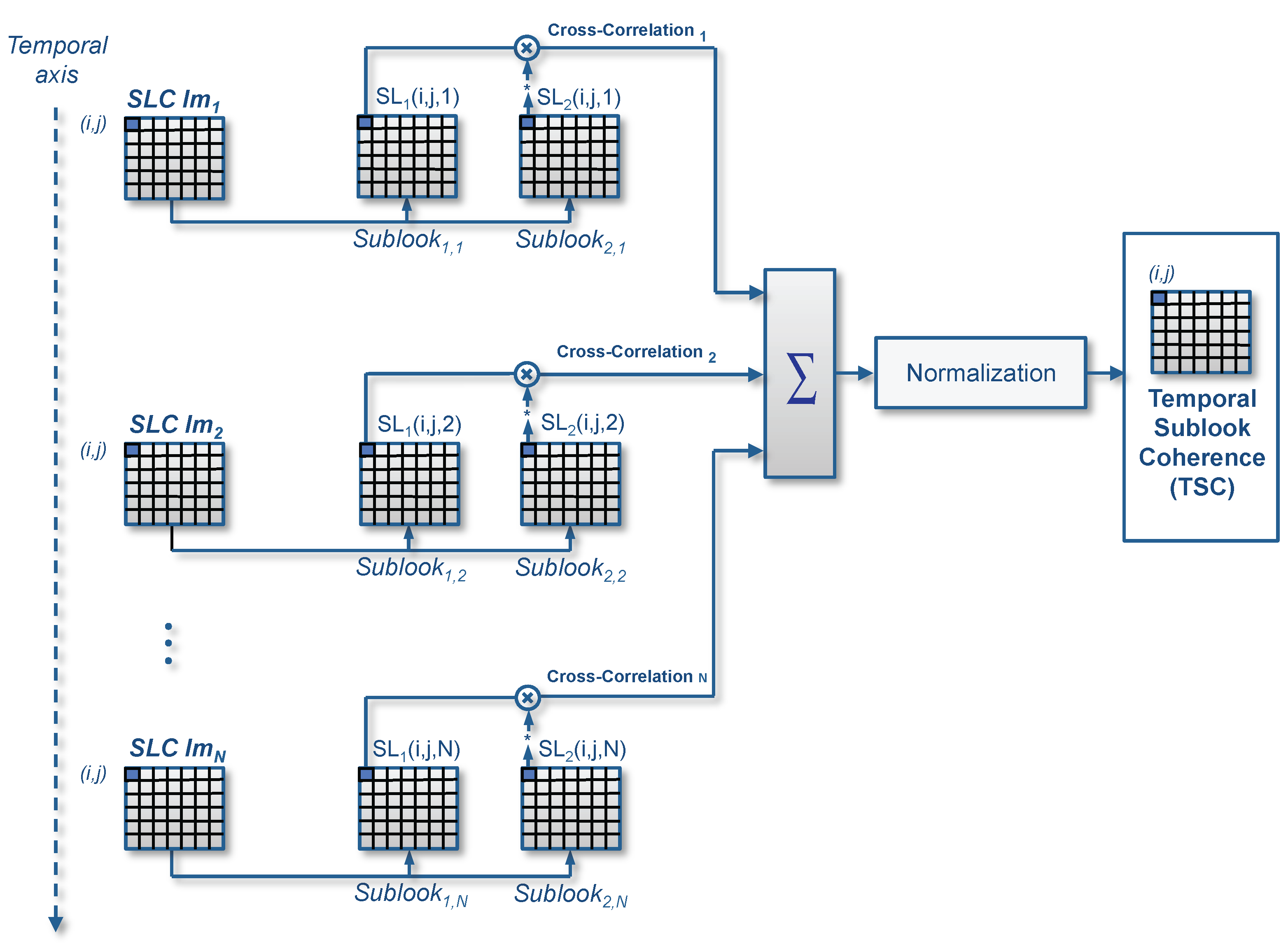
3. Sublook Generation and Temporal Sublook Coherence Evaluation

This Section presents a brief review of the TSC approach in order to ease the comprehension of the rest of the manuscript. The maps obtained by means of TSC are compared with the traditional phase quality estimators for the GB-SAR and TerraSAR-X datasets described in the previous section.

The objective of the TSC approach is to find the so-called SCS, which refers to those targets that behave as point-like scatterers in terms of the spectrum properties throughout the whole multi-temporal set of SAR images available [25]. This means looking for those targets characterized by a high correlated spectrum in range, azimuth and height for all of the acquisitions. Since some scatterers usually present a non-uniform azimuth scattering pattern, the assumption of the correlated spectrum is typically applied only in the range direction [26].

Working with the spectral properties of point-like scatterers presents clear advantages [25]. In contrast to the PS approach, the TSC is not affected by the possible amplitude fluctuations of point-like scatterers along the temporal axis. The amplitude, thus, plays no role in the TSC estimation, and for this reason, a radiometric calibration of data is not required. Moreover, the resolution of the images is better preserved in comparison with the coherence stability pixel selection approach. Only a loss of a factor of two is produced in the range direction due to the sublook generation process [26]. This resolution loss may be partially overcome using the spatial variant apodization (SVA) filtering technique, as suggested in [25,31]. Finally, due to the nature of the estimator, which is based on exploiting the coherence between different sublooks of the image spectrum, it allows reliable full-resolution detection capabilities, even when a few number of SAR images are at our disposal, as will be demonstrated throughout this manuscript.

The TSC evaluation requires, beforehand, a sublook generation process. A sublook may be defined as a spectrum portion of the full available system bandwidth. This process can be summarized in the following points [26]:

• First of all, the SLC spectrum must be unweighted. SAR images are typically filtered with linear windows in order to reduce the impact of side-lobes. Taking the sublooks directly from the taperedspectra may lead to unbalanced distributions of energy in the sublooks, which could have a negative impact during the later TSC evaluation.
• Once the image spectrum is unweighted, it is divided into two non-overlapping sublooks, which, at the same time, are base-banded to the same center frequency. This step is carried out in order to avoid linear phase terms during the TSC evaluation.
• Each sublook spectrum may be additionally weighted to reduce the side-lobes in the detection.
• An inverse Fourier transform is finally applied to each sublook in order to obtain them in the spatial domain.

Once the sublooks of each image are calculated, the TSC may be evaluated in order to detect SCS, which are directly related to the deterministic point-like scatterers within the area of interest.

Since a pixel-wise product in the space-domain translates into a spectrum correlation in the frequency-domain, the TSC is estimated employing the coherence estimator through the temporal axis among the sublook collections available [25]:

$$T\hat{S}C\left(i,j\right)=\frac{\left|{\displaystyle \sum _{n=1}^{N_{im}}S{L}_1\left(i,j,n\right)\cdot S{L}_2^{\ast }\left(i,j,n\right)}\right|}{\sqrt{{\displaystyle \sum _{n=1}^{N_{im}}{\left|S{L}_1\left(i,j,n\right)\right|}^2\cdot {\displaystyle \sum _{n=1}^{N_{im}}{\left|S{L}_2\left(i,j,n\right)\right|}^2}}}}$$

(1)

where SL₁ and SL₂ are the complex values from two pixels (i, j) of the first and the second sublook for each acquisition image n, and N_im refers to the total number of images. Notice how the spatial averaging used in the traditional approach [26] is now replaced by a temporal averaging [25]. Figure 5 represents the sketch of the TSC flow chart for a generic pixel (i, j).

Figure 5. Sketch of the TSC flow chart for a generic pixel (i, j).

Figure 5. Sketch of the TSC flow chart for a generic pixel (i, j).

Those targets exhibiting high values of TSC within the area of interest, will be directly referred to as SCSs and, consequently, will belong to the final selection of high-quality pixel candidates, or persistent scatterers, for the PSI processing [25].

At this stage, the accuracy of the TSC estimation needs to be commented on in further detail. The reliability of the TSC estimation depends on the number of independent samples involved in the estimation, i.e., the number of images [25]. In fact, the mathematical formulation to characterize the TSC estimation accuracy is totally equivalent to the one developed by Touzi and Lopes in [32] for the classical coherence estimator. The only difference is that now, the spatial averaging is replaced by a temporal one, as indicated above. The probability density function of the TSC magnitude estimator may hence be expressed as a function of the ‘true’ TSC absolute value and the number of temporal samples involved in the estimation [32]; see Figure 6. As happens with the coherence estimator, the TSC is a biased estimator. Its value is overestimated for low magnitudes of the ‘true’ TSC values and/or when the number of temporal samples, i.e., the number of SAR acquisitions involved in the estimation, is low. Since the estimation bias is smaller for high values of TSC, where the thresholds are typically set to detect the SCSs, a reliable estimation may be obtained even when a relatively reduced number of SAR images, around 10, is available. This fact provides the TSC estimator a competitive advantage with respect to the PS approach, which requires a larger number of images, typically more than 20, to reach reliable estimations of the D_A and, therefore, of the phase statistics.

Figure 6. (a) Expectation value and (b) standard deviation of the TSC estimation as a function of its “true” value, for different numbers of images.

Figure 6. (a) Expectation value and (b) standard deviation of the TSC estimation as a function of its “true” value, for different numbers of images.

Figure 7 and Figure 8 illustrate the performance of the TSC approach compared with the traditional phase quality estimators for both the ground-based and the orbital datasets described in Section 2, respectively. Figure 7a shows the TSC estimation, while Figure 7a,b shows the temporal mean coherence and the D_A maps, respectively, for the GB-SAR dataset. In parallel, Figure 8a,b,c show the same maps for the TerraSAR-X dataset. Since low D_A values correspond to the highest quality pixels, the color bar has been inverted for the latter. In addition, it is worth mentioning that when using large ML windows, especially with the new family of high-resolution X-band SAR sensors, many stable point-like targets surrounded by non-coherent clutter are unfortunately lost. In order to use the coherence estimator to make a cross-check with the other techniques, a 5 × 5 ML window has been used to preserve as much as possible the original resolution of images. This ML factor shows a good trade-off between the reliability of the coherence estimator and the preservation of the spatial resolution.

Figure 7. (a) TSC; (b) mean coherence; and (c) D_A maps over El Forn de Canillo test site for the GB-SAR dataset.

Figure 7. (a) TSC; (b) mean coherence; and (c) D_A maps over El Forn de Canillo test site for the GB-SAR dataset.

Figure 8. (a) TSC; (b) mean coherence; and (c) D_A maps over El Forn de Canillo test site for the sliding Spotlight TerraSAR-X dataset. The figures on the right represent a zoom of the area highlighted with a white rectangle in the figures on the left.

Figure 8. (a) TSC; (b) mean coherence; and (c) D_A maps over El Forn de Canillo test site for the sliding Spotlight TerraSAR-X dataset. The figures on the right represent a zoom of the area highlighted with a white rectangle in the figures on the left.

As seen before, El Forn de Canillo is mainly a vegetated area only containing a few man-made structures and rocky areas suitable for the PSI processing. In general, the highest quality points detected from all of the estimators correspond with these areas (reddish hue regions). All estimators follow the road, the buildings and the rocky and bare surfaces present in the area of interest for both sensors.

Going into further detail, some considerations deserve special attention. Notice how Figure 7b and Figure 8b evidence the loss of spatial resolution when employing the mean coherence approach. Despite the reduced ML factor employed (5 × 5), the resolution loss is evident for both sensors. This fact will lead to a significant loss of pixels and details in the later PSI processing, as shown later. Despite this negative aspect, notice how the ML carried out during the coherence estimation reduces the interferometric phase noise, and this fact is translated into a better identification of the persistent scatterers available with respect to the other estimators, which work at full resolution. Due to the intrinsic low-pass filtering related with the ML carried out during the coherence estimation, this approach shows the “cleanest” results. However, this does not mean that some high-quality points surrounded by non-coherent clutter have been lost. Furthermore, Figure 7c and Figure 8c show how the D_A estimator exhibits the worse performance in terms of detection capabilities. In general terms, the D_A estimator presents low values on the man-made structures, as it should be, but also on some low-quality vegetated regions, if compared with the TSC approach. This fact is more noticeable in the TerraSAR-X dataset, where the road in Figure 8c is hardly recognizable, presenting surrounding pixels with low D_A values. Notice how the TSC estimator better preserves the details and presents a better contrast between high-quality and low quality areas. As seen hereinafter, this fact will prevent the inclusion of outliers if the pixel selection thresholds are relaxed in order to improve the pixels’ density. This strategy is typically employed to obtain a sufficient network of pixels for reliable PSI processing when the number of high-quality pixels is low, as is the case of this work.

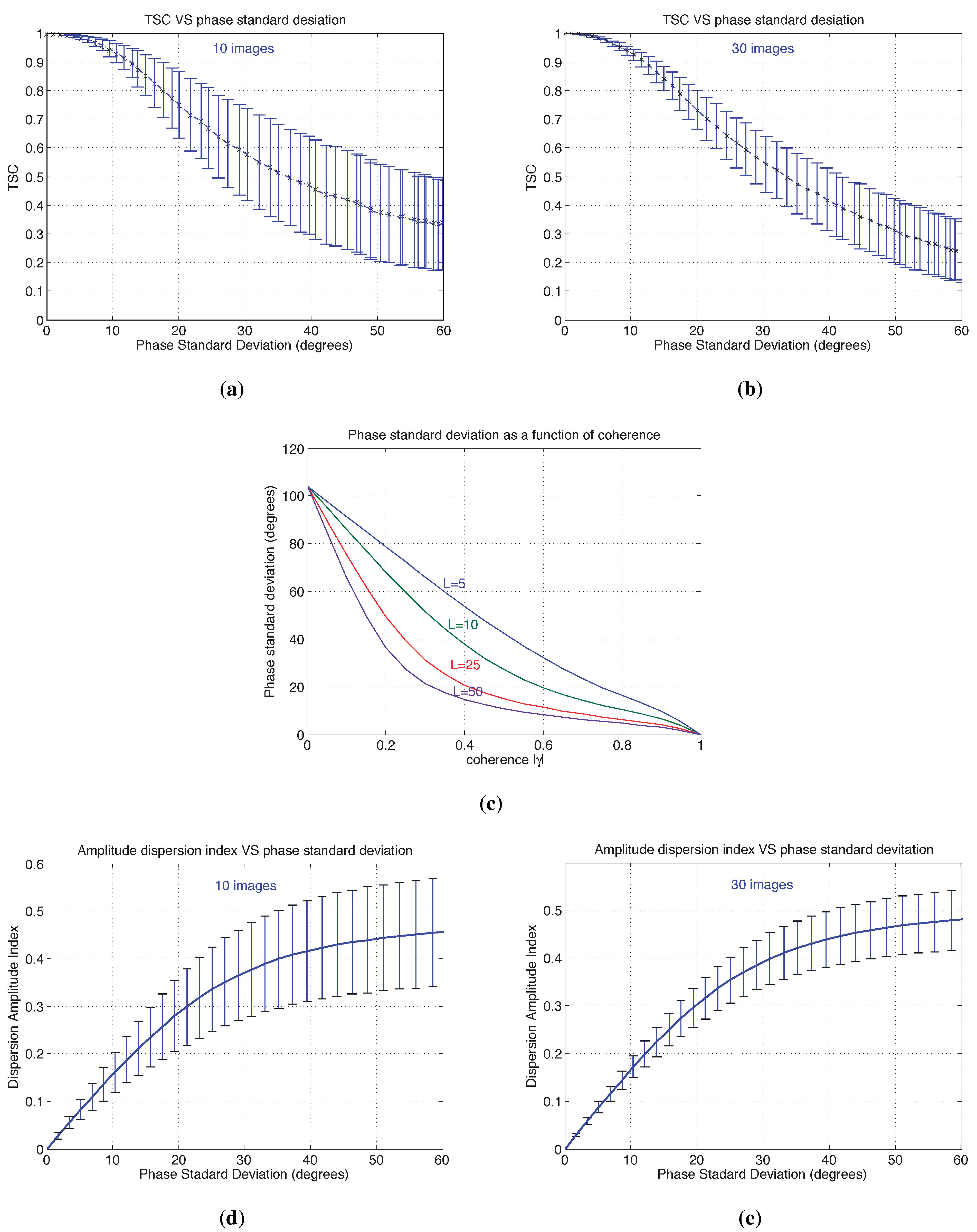
4. Phase Statistics and Pixel Selection Candidates

In order to to establish an adequate threshold to carry out a pixel section of persistent scatterers, the relationship between the TSC metrics and the pixels’ phase standard deviation should be calculated. As indicated in [25], this relationship may be obtained through the following simulation. First, a deterministic point-like scatterer is simulated in the spectrum domain, generating an ideal flat-shape function of unitary amplitude. This spectrum is hence corrupted by adding uncorrelated complex circular Gaussian noise in order to degrade its quality. The process is repeated for each image of a simulated dataset. At this point, the standard deviation of the added noise is gradually incremented from 0.05 to 0.95, and for each case, 5000 realizations are performed. The TSC is then calculated, and finally, the spectrum is inverse transformed to the temporal domain in order to evaluate the mean and temporal standard deviation of the target’s phase [25].

Figure 9a,b shows the relationship between the estimated TSC and the pixels’ phase standard deviation considering 10 images and 30 images, respectively. As seen in the analysis carried out during the estimation accuracy (Figure 6), a larger number of samples involved in the estimation yields to smaller error bars in the phase statistics estimation.

In order to establish equivalent thresholds during the pixel selection step and, thus, make a fair comparison among all methods, the same relationship is calculated for the coherence stability and the D_A approaches, as follows. Figure 9c illustrates the relationship between the estimated coherence and the phase standard deviation following the formulation presented by Touzi and Lopes in [32]. Likewise, Figure 9d,e, shows the relationship between the phase standard deviation and the amplitude dispersion index D_A derived by the numerical simulation stated in [6] considering 10 and 30 images being available, respectively. The values of dispersion in the estimation are represented by the vertical bars, while the solid line represents its mean value. Notice how, again, the quality of the D_A estimation depends on the number of images available, the error bars for the case of having 10 SAR images available being considerably larger.

At this stage, all estimators have been related to the target’s phase statistics. An adequate threshold may now be established in order to ensure a specific phase stability during the PSI processing.

Figure 10 and Figure 11 show a comparison in terms of pixels selected between the TSC approach and the classical techniques for the GB-SAR and the TerraSAR-X datasets, respectively. In order to ensure a fair comparison, equivalent thresholds over the phase quality estimators have been established in order to provide the same requirements in terms of phase dispersion according to Figure 9. A threshold of 0.82, which corresponds to a phase standard deviation of roughly 15° (see Figure 9a) has been fixed to the TSC approach. In parallel, a threshold of 0.65 considering a 5×5 ML [32] (see Figure 9c) has been fixed to the mean coherence, and finally, a threshold of 0.25 has been applied to the D_A [6] (see Figure 9d) to produce the same response in terms of phase standard deviation. Figure 12 gives the same information in terms of the number of pixels selected. Notice how the pixels selected with the coherence and the TSC approach correspond with the persistent scatterers present in the area of interest for both datasets, since they perfectly fit the road, the man-made structures and the few rocky and bare surfaces within the illuminated scenario. Notice the resolution loss inherent to the coherence approach, which leads to a reduced number of pixels compared with the TSC and D_A approaches (roughly four-times less). As expected from the study carried out in the previous section, the PS approach provides a greater number of selected pixels (roughly 10 percent more), but including a significant amount of unreliable ones selected over vegetated areas, which are characterized by a high phase dispersion index; see Figure 10 and Figure 11. As seen, the reduced number of SAR images available yields to a poor D_A estimation. At this time, it may be thought that this large number of unreliable pixels identified could be reduced restricting the D_A threshold to lower values, which is only partially true. Figure 11d corresponds to the selection of pixel candidates for the TerraSAR-X dataset employing a more restricted D_A threshold (0.15, which corresponds to 10° of phase standard deviation). Indeed, almost all of the outliers have disappeared, but the density over the persistent scatterers available has been also drastically reduced. The road and the man-made structures clearly identified in Figure 11a,b are now diluted and hardly detected.

The study carried out in this section evidences once more that a minimum number of 20 images is required in order to produce a reliable D_A estimation. Contrarily, the TSC approach performs well, even when a small dataset of SAR images is available.

Figure 9. Relationship between TSC and phase standard deviation considering (a) 10 and (b) 30 SAR images; (c) phase standard deviation as a function of coherence for different numbers of multi-look (ML) factors; comparison of the amplitude dispersion index D_A and the phase standard deviation (in degrees) as a function of noise computed by numerical simulation considering (d) 10 and (e) 30 SAR images available.

Figure 9. Relationship between TSC and phase standard deviation considering (a) 10 and (b) 30 SAR images; (c) phase standard deviation as a function of coherence for different numbers of multi-look (ML) factors; comparison of the amplitude dispersion index D_A and the phase standard deviation (in degrees) as a function of noise computed by numerical simulation considering (d) 10 and (e) 30 SAR images available.

Figure 10. Pixel candidates selected using (a) the TSC with a threshold of 0.82; (b) the coherence stability with a threshold of 0.65; and (c) the D_A with a threshold of 0.25 for the GB-SAR dataset.

Figure 10. Pixel candidates selected using (a) the TSC with a threshold of 0.82; (b) the coherence stability with a threshold of 0.65; and (c) the D_A with a threshold of 0.25 for the GB-SAR dataset.

Figure 11. Pixel candidates selected using (a) the TSC with a threshold of 0.82; (b) the coherence stability with a threshold of 0.65; and the D_A with a threshold (c) of 0.25 and (d) of 0.15 for the TerraSAR-X dataset.

Figure 11. Pixel candidates selected using (a) the TSC with a threshold of 0.82; (b) the coherence stability with a threshold of 0.65; and the D_A with a threshold (c) of 0.25 and (d) of 0.15 for the TerraSAR-X dataset.

Figure 12. Number of pixel candidates selected using the TSC, the coherence stability and the D_A approaches for (a) the GB-SAR and (b) the TerraSAR-X datasets.

Figure 12. Number of pixel candidates selected using the TSC, the coherence stability and the D_A approaches for (a) the GB-SAR and (b) the TerraSAR-X datasets.

5. PSI by Means of TSC: Results and Discussion

This section presents the PSI displacement maps obtained with the TSC approach on the test site corresponding to the landslide of El Forn de Canillo for the GB-SAR and the TerraSAR-X datasets described in Section 2. A close comparison, in terms of pixel density and phase quality, with the traditional coherence stability and D_A approaches, is put forward. Finally, some ground-truth data are also presented in order to validate the PSI results obtained.

Beforehand, some remarks about GB-SAR and sliding spotlight interferometry are briefly introduced. The principal steps of the coherent pixel technique (CPT) technique are also reviewed in order to ease the comprehension of the PSI displacement retrieval process employed in this study.

5.1. Interferometric Processing Chain Considerations and CPT Overview

5.1.1. GB-SAR Interferometry

Prior to applying any PSI technique, a pre-processing of GB-SAR data must be carried out in order to improve the quality of the SAR images corresponding to each measurement day and to compensate for the APS present in the long-time interferograms corresponding to the different measurement campaigns.

Considering a total of N daily datasets, each one composed of M_i zero-baseline GB-SAR raw images, with 1 ≤ i ≤ N , the process may be summarized in the following two blocks [33]:

• The first block, referred to as short-term processing (STP) [33], basically consists of two steps.
  The first one is based on carrying out the focus of the raw data. On the one hand, since the RiskSAR-X sensor is based on a LFM-CW radar, the range compression can be carried out with a simple FFT of the time-domain deramped received signal [34,35]. On the other hand, since the cross-range resolution is not constant due to the limited length of the synthetic aperture of GB-SAR sensors, the back-projection technique proved to be the most suited for the azimuth focusing [34]. Once the images has been focused, a temporal averaging of each daily dataset, composed of M_i zero-baseline acquisitions corresponding to the same measurement day i, is carried out in order to improve the SNR of time-stationary targets, leading to a higher quality time-averaged SLC image from each daily dataset corresponding to each measurement campaign. For the dataset used in this paper, 10 time-averaged SLC images will be finally available after this step.
• The following step, referred to as long-term processing (LTP), consists of compensating for the APS present between the different time-averaged SLC images obtained in the previous STP block. From all of the methods available in the literature [33,36,37,38], the RiskSAR-X makes use of model-based solutions [33]. This kind of solution proved to be very effective, reaching very good performances with no use of extra meteorological data or stable ground control point (GCP) information. The APS estimation and compensation process is a key issue in GB-SAR processing in order to obtain a reliable set of APS-free interferograms suitable for the PSI processing. For the dataset used in this paper, 45 APS-free interferograms are finally available. Finally, to face temporal decorrelation phenomena and enhance the phase quality of interferograms, the processing can be benefited by the exploitation of polarimetric information, such as the one provided by the RiskSAR-X sensor. In classical PSI, only a single-polarimetric channel is considered for the processing. This means that all pixels involved in PSI algorithms belong to the same polarimetric channel. In this context, polarimetric optimization techniques may be employed in order to improve the phase quality of interferograms [39].

5.1.2. Spotlight SAR Interferometry

The azimuth resolution of a SAR image is mainly determined by the characteristics of the azimuth radiation pattern of the antenna. In the conventional strip-map mode, the resolution is roughly half the azimuth length of the antenna and the processing parameters, Doppler centroid and Doppler rate, are azimuth invariant. In this context, the antenna length cannot be arbitrarily reduced without the risk of causing azimuth and/or range ambiguities.

In the sliding spotlight mode, the antenna pointing is constantly steered to maintain the radar footprint illuminating a fixed area on the ground during a time period longer than the conventional SAR aperture interval, thus achieving an azimuth resolution improvement. The steering of the antenna causes the spotlight raw data, as well as the focused image to present a systematic Doppler centroid drift in the azimuth direction. This drift rate f_DR of the image spectrum may be calculated from the Doppler values and their zero-Doppler time differences through the first and last azimuth time of the focused scene as follows [30]:

$$f_{DR}=\frac{f_{DC,n}-f_{DC,1}}{t_{DC,n}-t_{DC,1}}$$

(2)

where f_DC,1 and f_DC,n account for the first and the last Doppler annotated values in the product and t_DC,1 and t_DC,1, their correspondent zero-Doppler corrected times.

This characteristic must be taken into account in the following interferometric processing chain steps: co-registration, resampling and, when applied, common band filtering. Prior to applying these steps, the center frequency of the interpolation kernels in azimuth must consider the Doppler drift or images must be adequately base-banded.

Each azimuth line must hence be demodulated with the following chirp function parameterized with drift rate [30]:

$$c\left(t\right)=e^{-j\pi {\left(t-t_{start}\right)}^2{f}_{DR}}$$

(3)

where t_start refers to the azimuth start time of the scene.

Once the drift rate is removed, the spectrum is centered on the start Doppler value. Then, the base-banding is performed, as is in the traditional strip-map case, multiplying the image in the spatial domain by a phase ramp in the azimuth parameterized with the zero-Doppler start value. The co-registration, resampling and common band filtering can be now applied. After these steps, both scenes are modulated back to their original frequency bands by multiplying them with the conjugate chirp c*(t), and classical strip-map PSI techniques may be employed.

5.1.3. The Coherent Pixels Technique

Among the multiple advanced PSI techniques developed in the last decade by the SAR community [5,6,7,8,9,10,11,12,13,14,15], the CPT [18,40] has been employed in this work to carry out the PSI processing.

This technique has been widely exploited during the last decade for studying the temporal evolution of a large number of ground displacements caused by human activities and natural hazards, using SAR data collected by space-borne sensors. The CPT allows the estimation of the linear and non-linear components of displacement, the topographic error of the digital elevation model (DEM) used in the generation of the differential interferograms and the APS from a set of differential interferograms [18,40]. In this framework, the CPT has been recently adapted to work with the zero-baseline fully-polarimetric GB-SAR data provided by the RiskSAR-X sensor. In addition, the TSC approach has been integrated in the pixel selection block, which worked before with the coherence stability and PS approaches.

Once the pixel selection is carried out, the first step of the CPT algorithm consists of performing a Delaunay triangulation of the pixel candidates selected. This strategy allows one to work with phase increments between pixels instead of absolute phases, which present some advantages. On the one hand, the absolute phase of individual pixels is not of practical utility due to the presence of different phase offsets among the set of differential interferograms. On the other hand, it allows minimizing the APS present in interferograms. Finally, if a good distribution of pixel candidates is assumed, the absolute phase increments may be supposed in most of the interferograms to be lower than π radians. The phase unwrapping step may hence be skipped at this stage.

Under the more general approach considering non-zero baseline interferograms, which applies to space-borne SAR data, the interferometric phase increment Δφ_m,n between two connected points P_m and P_n by the triangulation is expressed for the i−th interferogram as [18,40]:

$$\Delta {\phi }_{m,n}\left(T_i,B_{n,i}\right)=\frac{4\pi }{\lambda }\cdot T_i\cdot \left(v\left(x_m,y_m\right)-v\left(x_n,y_n\right)\right)+\frac{4\pi }{\lambda }\cdot \frac{B_{n,i}}{R_i\sin {\theta }_i}\cdot \left(\epsilon \left(x_m,y_m\right)-\epsilon \left(x_n,y_n\right)\right)+\Delta {\phi }_{m,n}^{res}$$

(4)

where (x_m, y_m) and (x_n, y_n) refer to the coordinates of the nodes forming the arc_m,n, v(x_m, y_m) − v(x_n, y_n) and ε(x_m, y_m) − ε(x_n, y_n) account for the increment of linear displacement rate and topographic error, λ indicates the wavelength, T_i and B_n,i are the temporal and spatial baselines, respectively, R_i is the sensor to target distance, θ_i the incidence angle and $\Delta {\phi }_{m,n}^{res}$, referred to as residual phase, refer to the atmospheric, non-linear and noise components of the phase.

For GB-SAR sensors operating under a zero-baseline configuration, the topographic error phase term is not considered. Likewise, there is not any APS contribution in the residue, since it was compensated for previously. The interferometric phase increment expression seen in Equation (4) is hence simplified in the following way:

$$\Delta {\phi }_{m,n}\left(T_i\right)=\frac{4\pi }{\lambda }\cdot T_i\cdot \left(v\left(x_m,y_m\right)-v\left(x_n,y_n\right)\right)+\Delta {\phi }_{m,n}^{res}$$

(5)

where, now, $\Delta {\phi }_{m,n}^{res}$ accounts only for the non-linear and noise components of the phase.

In order to retrieve the displacement rate, a linear model is defined for each arc of the triangulation. The model is then adjusted to data through the minimization of a cost function, referred to as model adjustment function (MAF). Once the linear displacement rate is obtained, the MAF is evaluated in order to measure the quality of each arc. At this stage, low quality arcs are truncated, and those pixels which remain disconnected are removed. Another, the iteration of the minimization process is carried out with the surviving pixels. The process removes the pixels that do not fit the linear model, which may be caused by strong non-linear displacements in some particular cases. Finally, the absolute values of linear displacement for each pixel are obtained through an integration process, using one or multiple seeds with known behavior as tie points [40].

Finally, it must be pointed out that, regardless of the platform (orbital-, airborne- or ground-based), SAR systems only have sensitivity in the LOS direction. When facing landslide monitoring applications, the real displacement produced has an intrinsic topographic dependence, being related to the local slopes of the area under study. With no a priori knowledge, the more realistic kinetic model is based on considering that the surface mostly moves along the steepest gradient of the terrain slope. This information may be obtained from a DEM of the illuminated area. For this reason, results must be down-slope projected prior to its interpretation. Once the displacement vectors are accordingly projected, they are geocoded in map coordinates and may be visualized by using Geographical Information System (GIS) software or a virtual globe viewer.

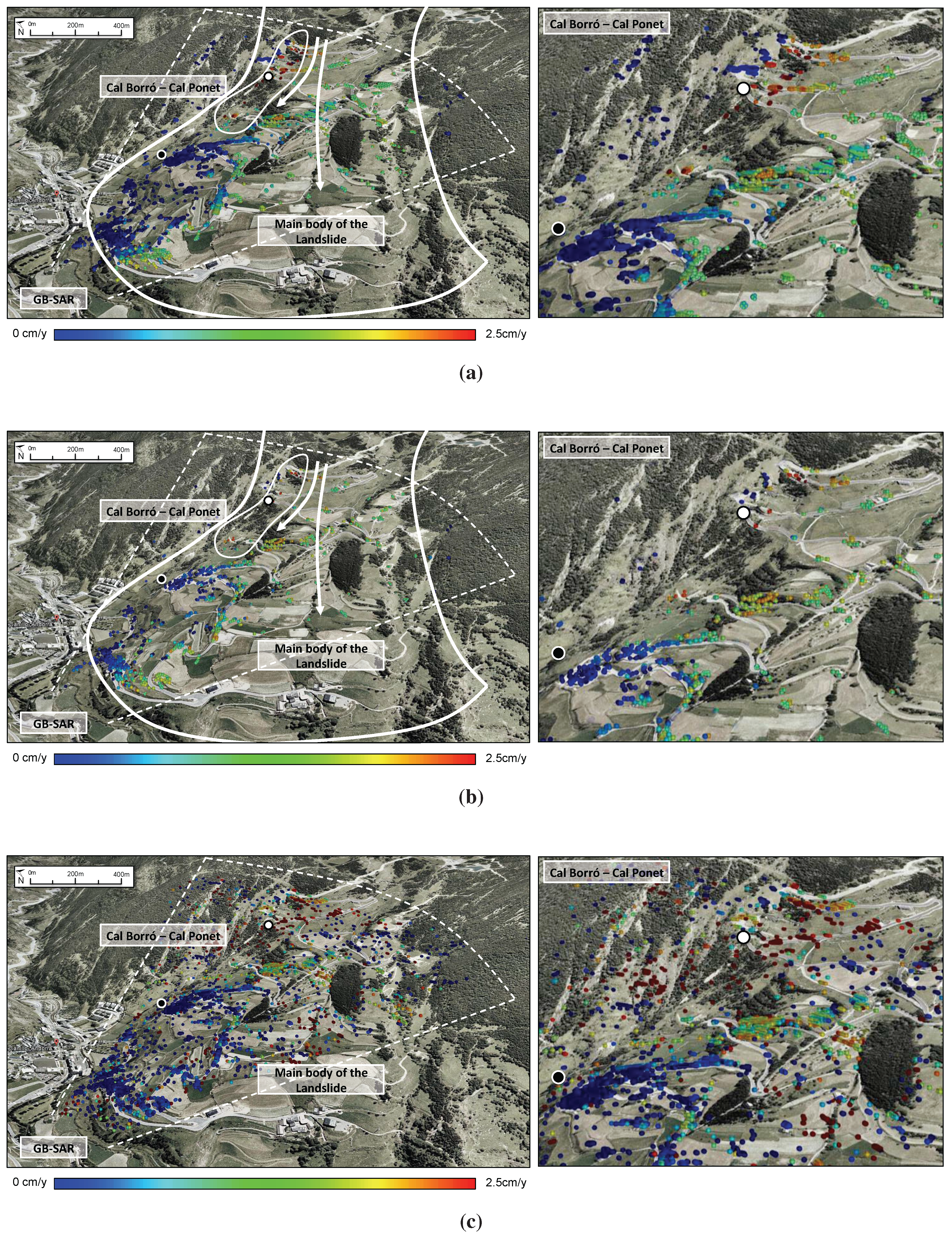
5.2. PSI Displacement Results

Figure 13 and Figure 14 show the down-slope ground displacement maps of El Forn de Canillo geocoded over a Google Earth image for the RiskSAR-X and the TerraSAR-X datasets, respectively. For the coherence stability method, a threshold of 0.65 has been employed; the PS technique has been carried out using a D_A threshold of 0.25; and finally, a threshold of 0.82 has been employed for the TSC approach. These thresholds are set in order to ensure the use of pixels with similar phase standard deviations in all cases, as seen in the previous section.

Figure 13. Geocoded down-slope linear displacement corresponding to El Forn de Canillo using (a) the TSC, (b) the coherence stability and (c) the D_A approach for the GB-SAR dataset. The black spot indicates the location of the seed employed during the integration step. The white spot indicates the location of the inclinometer S10, which will be employed as ground-truth to validate the results.

Figure 13. Geocoded down-slope linear displacement corresponding to El Forn de Canillo using (a) the TSC, (b) the coherence stability and (c) the D_A approach for the GB-SAR dataset. The black spot indicates the location of the seed employed during the integration step. The white spot indicates the location of the inclinometer S10, which will be employed as ground-truth to validate the results.

Figure 14. Geocoded down-slope linear displacement corresponding to El Forn de Canillo using (a) the TSC and (b) the coherence stability approach for the TerraSAR-X dataset. The black spot indicates the location of the seed employed during the integration step. The white spot indicates the location of the inclinometer S10, which will be employed as ground-truth to validate the results.

Figure 14. Geocoded down-slope linear displacement corresponding to El Forn de Canillo using (a) the TSC and (b) the coherence stability approach for the TerraSAR-X dataset. The black spot indicates the location of the seed employed during the integration step. The white spot indicates the location of the inclinometer S10, which will be employed as ground-truth to validate the results.

First of all, notice how the results in the common area processed by both sensors show a high agreement. As expected, the TSC and the coherence stability approaches are retrieving similar deformation trends, except for the increase in pixel density, especially over the land covers characterized by rocks surrounded by vegetation, which may be appreciated at both sides of the landslide. Recall that the ML processing limits the selection of deterministic point-like scatterers surrounded by non-coherent clutter. The denser results benefit the construction of a more robust network during the minimization and integration processes of the CPT, thus improving the reliability of the PSI results. At a more detailed level, it must be noticed that the displacement magnitudes obtained by means of the TSC approach reach slightly higher values of displacements compared with the coherence stability results. This difference may be produced by ML carried out during the coherence estimation, which leads to averaging the displacement within the multilooked area.

Although the studies reported throughout the paper prevent the employment of the D_A estimator to perform the pixels selection, a PSI processing has been carried out employing the D_A for the GB-SAR study case. Indeed, the displacement results provided by the PS approach clearly result in being unreliable due to the low number of images available (see Figure 13c) and present a large amount of outliers.

Regarding the interpretation of the displacement maps retrieved, notice how in the lower part of the landslide, the PSI results obtained show a high agreement with the conclusions extracted from the field monitoring campaigns made between 2007 and 2009 presented in [28] (reviewed in Section 2). The displacement maps obtained reveal that the main body of landslide experienced a residual movement of 1–1.5 cm during the measurements interval. In addition, the local slide of Cal Borró-Cal Ponet may be perfectly identified for both sensors, presenting a higher activity of 2–2.5 cm/year.

Finally, some displacement trends, unknown until now, are also revealed in the upper part of the El Forn de Canillo through the TerraSAR-X PSI processing: the crest linking the Pic del Maians to the Pic d’Encampadana and another closer to the area known as Pla del Géspit. These displacements detected exhibit displacements closer to ~3 cm/year. Unfortunately, the upper part of El Forn de Canillo lacks instruments to compare and validate the measurements obtained with TerraSAR-X. Despite this, the magnitude of displacement rates suggests that the slope should show activity indicators. Some field inspections have been carried out confirming the existence of such indicators as structural disturbance, tension cracks, depressions filled with sediments, covered by vegetation, as well as tilted and rotated blocks, with weathered surfaces.

At this stage, some ground-truth data are presented in order to validate the PSI results obtained. Figure 15 shows the inclinometric results in the borehole S10, which corresponds to the maximum displacement rate area of the lower part of the landslide (Cal Borró-Cal Ponet). The location of the borehole S10 is indicated in Figure 1b, seen in Section 2. In addition, this location has been also highlighted with a white spot in the PSI result figures (Figure 13 and Figure 14).

Inclinometers are geotechnical devices for measuring horizontal displacements affecting the shape of a guide casing embedded in the ground. They provide the displacements undergone in two orthogonal planes, and this information allows obtaining the real 3D ground displacement vector of movement. It is worth mentioning that in order to obtain reliable estimations, the end of the guide casing must reach a stable reference. The technique consists of obtaining relative displacements profiles over time by repeating measurements at the same depths. This measures may be compared in order to detect the possible displacements undergone along the different measurement campaigns. Moreover, recording the magnitude of displacements at different reading depths is useful to identify shear bands and different units of movement. The most common way to analyze inclinometric results is based on displaying the cumulative lateral displacement along different depths, starting at the bottom of the casing and integrating increments of displacement for all depths up to the ground surface.

Figure 15. Inclinometric results in the borehole S10 (Cal Borró-Cal Ponet).

Figure 15. Inclinometric results in the borehole S10 (Cal Borró-Cal Ponet).

Figure 15 illustrates the deformed shape of the inclinometer casing along the borehole for different periods. Concretely, the curves available correspond to the period from December 2010, to October 2011, all referring to July 2008. The profiles plotted correspond to the maximum displacement axis (down-slope direction). Since the displacement is produced along the steepest gradient of the slope, the orthogonal axis did not record any displacement, and for this reason, it has not been represented in the figure. As indicated by the S-shaped plot, the main shear band is located at roughly 30 m under the surface of the landslide. The upper part of the plot has been amplified to compare the inclinometric results with the ones obtained using PSI techniques. The displacement undergone by the inclinometer between the period corresponding from December 2012 to October 2013, coinciding with the PSI processing, corresponds to 1.8 cm. Since the inclinometric results are given in an horizontal plane, these must be divided by the cosine of the slope angle in this area (~20°) in order to obtain the total down-slope displacement ~ 1.8 cm/cos(20°) = 1.91 cm. This is equivalent to a total of roughly 2.3 cm/year. The results provided by the SAR sensors register ~2.5 cm/year in this region, thus showing high agreement with the ground truth available.

As mentioned above, some geological evidence observed recently also corroborates the displacement results retrieved. Figure 16 presents some photographs obtained during several field inspections carried out during 2013–2014. Figure 16a shows a picture of the interior of a famous house built in the mid-nineteenth century, near the area of maximum displacement of Cal Borró-Cal Ponet. The curved shape of the wall evidences the presence of displacements in the area. Figure 16b shows a picture of several cracks and shear openings along the road pavement, which have also appeared close to this area. Figure 16c shows curved trunks belonging to trees that have been subjected to a progressive tilt at the base, forcing the trunk to adopt this curvature in order to point vertically. These photographs have been taken in the upper part of the landslide. Figure 16d illustrates fresh cracks and openings within the rock mass in the outcrops of the Clots Fondos area, which denote the current activity. Figure 16e shows the detail of the perimeter stone fence that surrounds the area of Prat del Fornet field. The waviness of the formerly straight wall evidences the movements developing in the area.

Figure 16. Photographs obtained during the field inspections works carried out during 2013–2014 evidencing the activity of El Forn de Canillo. (a) Interior view of the cracked walls of a small farmhouse and (b) cracks along road pavement located close to the area of Cal Borró–Cal Ponet; (c) curved trunks belonging to trees that have been subjected to a progressive tilt; (d) fresh cracks and openings within the rock mass in the outcrops of the Clots Fondos area; (e) perimeter stone fence that surrounds the area of Prat del Fornet field.

Figure 16. Photographs obtained during the field inspections works carried out during 2013–2014 evidencing the activity of El Forn de Canillo. (a) Interior view of the cracked walls of a small farmhouse and (b) cracks along road pavement located close to the area of Cal Borró–Cal Ponet; (c) curved trunks belonging to trees that have been subjected to a progressive tilt; (d) fresh cracks and openings within the rock mass in the outcrops of the Clots Fondos area; (e) perimeter stone fence that surrounds the area of Prat del Fornet field.

As illustrated throughout the paper, the coherence stability and the TSC approach are more suitable when a low number of images are at our disposal. Contrarily, the PS approach fails under these boundary conditions due to the unreliable estimation of the D_A. In general terms, it behaves in a similar way compared to the other two methods, but the selection of unreliable pixels as persistent scatterers finally leads to a noisy displacement map with a large number of outliers. The improvement in terms of pixel density provided by the TSC approach with respect to the coherence stability approach hence increases the precision in determining the extension of the deformation and presents clear advantages for characterizing the behavior of the different local slides present in the area of study. These results reveal that the TSC approach presented overcomes the intrinsic limitations of the classical pixel selection approaches: it allows performing a reliable full-resolution pixel selection when a small number of SAR images is available.

6. Conclusions

This paper shows the application of the TSC approach to work over reduced datasets of SAR acquisitions. The performance of this novel estimator has been tested over the slow-moving landslide of El Forn de Canillo using 10 images collected at the X-band during a one-year measurement campaign using the UPC’s LFM-CW GB-SAR sensor. To complete the study, 10 sliding spotlight TerraSAR-X acquisitions have been also employed for the study. The type of data and the scenario selected has provided some added value to this work. The test site, mostly vegetated and only containing a few man-made structures, has constituted an extra challenge for the technique. PSI techniques usually perform worse over areas dominated by high temporal decorrelation phenomena.

The estimation accuracy, the number of pixel candidates and the final PSI displacement maps retrieved by means of the TSC approach proposed have been widely discussed in terms of pixel density and reliability. Furthermore, they have been compared with the so-called classical approaches, showing an improved performance on reduced datasets of SAR images. The number of pixels selected with the coherence stability and the TSC approach have been perfectly associated with the man-made structures and rocky areas present in the scenario. Both approaches have shown a similar performance in terms of PSI displacement results. Nonetheless, the resolution loss inherent to the coherence approach has led to a reduced number of pixels compared with the TSC approach (four-times less). Having higher densities in PSI results is a key factor, since it increases the precision of determining the extension of local displacements patterns and eases the characterization of the global displacement behavior. The PS approach has provided slightly higher pixel densities (roughly 10 percent more), but at the expense of including outliers in the final PSI results due to the unreliable estimation of the D_A index. In fact, it is a false improvement, as the low number of images makes the selection untruthful.

RiskSAR-X and TerraSAR-X have provided consistent measurements of the landslide displacements in El Forn de Canillo, which are compatible with the available inclinometric ones. Furthermore, the observations with TerraSAR-X, with greater spatial coverage, have shown that the displacements are significantly higher in the upper part of the slope (~3 cm/year), defining eventually an unstable rock mass whose existence had remained unnoticed so far. Field surveys have confirmed the presence of activity indicators in this area, such as recent depressions, structural disturbance and open tension cracks.

In conclusion, the TSC approach has been demonstrated to be an excellent choice to overcome the limitations of classical approaches, when the full-resolution of images is to be preserved and the number of SAR images available is low.

References

1. Massonnet, D.; Feigl, K.L. Radar interferometry and its application to changes in the Earth’s surface. Rev. Geophys. 1998, 36, 441–500. [Google Scholar] [CrossRef]
2. Bürgmann, R.; Rosen, P.A.; Fielding, E.J. Synthetic Aperture Radar interferometry to measure Earth’s surface topography and its deformation. Ann. Rev. Earth Planet. Sci. 2000, 28, 169–209. [Google Scholar] [CrossRef]
3. Gabriel, A.K.; Goldstein, R.M.; Zebker, H.A. Mapping small elevation changes over large areas: Differential radar interferometry. J. Geophys. Res. 1989, 94, 9183–9191. [Google Scholar] [CrossRef]
4. Hanssen, R.F. Radar Interferometry: Data Interpretation and Error Analysis; Kluwer Academic Publishers: Dordrecht, The Netherlands, 2001. [Google Scholar]
5. Ferretti, A.; Prati, C.; Rocca, F. Nonlinear subsidence rate estimation using permanent scatterers in differential SAR interferometry. IEEE Trans. Geosci. Remote Sens. 2000, 38, 2202–2212. [Google Scholar] [CrossRef]
6. Ferretti, A.; Prati, C.; Rocca, F. Permanent Scatterers in SAR interferometry. IEEE Trans. Geosci. Remote Sens. 2001, 39, 8–20. [Google Scholar] [CrossRef]
7. Mora, O.; Mallorqui, J.J.; Duro, J. Generation of deformation maps at low resolution using differential interferometric SAR data. In Proceedings of 2002 IEEE International Geoscience and Remote Sensing Symposium, IGARSS ’02. Toronto, ON, Canada, 24–28 June 2002.
8. Berardino, P.; Fornaro, G.; Lanari, R.; Sansosti, E. A new algorithm for surface deformation monitoring based on small baseline differential SAR interferograms. IEEE Trans. Geosci. Remote Sens. 2002, 40, 2375–2383. [Google Scholar]
9. Werner, C.; Wegmuller, U.; Strozzi, T.; Wiesmann, A. Interferometric point target analysis for deformation mapping. In Proceedings of 2003 IEEE International Geoscience and Remote Sensing Symposium, IGARSS ’03. Toulouse, France, 21–25 July 2003.
10. Arnaud, A.; Adam, N.; Hanssen, R.; Inglada, J.; Duro, J.; Closa, J.; Eineder, M. ASAR ERS interferometric phase continuity. In Proceedings of 2003 IEEE International Geoscience and Remote Sensing Symposium, IGARSS ’03. Toulouse, France, 21–25 July 2003.
11. Hooper, A.; Zebker, H.; Segall, P.; Kampes, B. A new method for measuring deformation on volcanoes and other natural terrains using InSAR persistent scatterers. Geophys. Res. Lett. 2004, 31. [Google Scholar] [CrossRef]
12. Lanari, R.; Mora, O.; Manunta, M.; Mallorqui, J.J.; Berardino, P.; Sansosti, E. A small-baseline approach for investigating deformations on full-resolution differential SAR interferograms. IEEE Trans. Geosci. Remote Sens. 2004, 42, 1377–1386. [Google Scholar] [CrossRef]
13. Hooper, A. A multi-temporal InSAR method incorporating both persistent scatterer and small baseline approaches. Geophys. Res. Lett. 2008, 35. [Google Scholar] [CrossRef]
14. Fornaro, G.; Reale, D.; Serafino, F. Four-dimensional SAR imaging for height estimation and monitoring of single and double scatterers. IEEE Trans. Geosci. Remote Sens. 2009, 47, 224–237. [Google Scholar] [CrossRef]
15. Ferretti, A.; Fumagalli, A.; Novali, F.; Prati, C.; Rocca, F.; Rucci, A. A new algorithm for processing interferometric data-stacks: SqueeSAR. IEEE Trans. Geosci. Remote Sens. 2011, 49, 3460–3470. [Google Scholar] [CrossRef]
16. Massonnet, D.; Briole, P.; Arnaud, A. Deflation of Mount Etna monitored by spaceborne radar interferometry. Nature 1995, 375, 567–570. [Google Scholar] [CrossRef]
17. Lundgren, P.; Usai, S.; Sansosti, E.; Lanari, R.; Tesauro, M.; Fornaro, G.; Berardino, P. Modeling surface deformation observed with synthetic aperture radar interferometry at Campi Flegrei caldera. J. Geophys. Res. 2001, 106, 19355–19366. [Google Scholar] [CrossRef]
18. Mora, O.; Mallorqui, J.; Broquetas, A. Linear and nonlinear terrain deformation maps from a reduced set of interferometric sar images. IEEE Trans. Geosci. Remote Sens. 2003, 41, 2243–2253. [Google Scholar] [CrossRef]
19. Kwok, R.; Fahnestock, M. Ice sheet motion and topography from radar interferometry. IEEE Trans. Geosci. Remote Sens. 1996, 34, 189–200. [Google Scholar] [CrossRef]
20. Refice, A.; Bovenga, F.; Guerriero, L.; Wasowski, J. DInSAR applications to landslide studies. In Proceedings of IEEE 2001 International Geoscience and Remote Sensing Symposium, IGARSS ’01. Sydney, Australia, 9–13 July 2001.
21. Kim, S.-W.; Won, J.-S. Measurements of soil compaction rate by using JERS-1 SAR and a prediction model. IEEE Trans. Geosci. Remote Sens. 2003, 41, 2683–2686. [Google Scholar] [CrossRef]
22. Buckreuss, S.; Balzer, W.; Muhlbauer, P.; Werninghaus, R.; Pitz, W. The terraSAR-X satellite project. In Proceedings of 2003 IEEE International Geoscience and Remote Sensing Symposium, IGARSS ’03. Toulouse, France, 21–25 July 2003.
23. Buckreuss, S.; Roth, A. Status Report on the TerraSAR-X Mission. In Proceedings of 2008 IEEE International Geoscience and Remote Sensing Symposium, IGARSS 2008. Boston, MA, USA, 7–11 July 2008.
24. Venturini, R.; Fois, F.; Sirocchi, G.; Bauleo, A.; Bazzoni, A.; Borgarelli, L.; Capece, P.; Cereoli, L.; Croci, R.; Farina, C.; et al. Experimental verification of COSMO-SkyMed SAR capabilities. In Proceedings of 2008 IEEE Radar Conference, RADAR ’08. Rome, Italy, 26–30 May 2008.
25. Iglesias, R.; Mallorqui, J.J.; Lopez-Dekker, P. DInSAR pixel selection based on sublook spectral correlation along time. IEEE Trans. Geosci. Remote Sens. 2014, 52, 3788–3799. [Google Scholar] [CrossRef]
26. Schneider, R.; Papathanassiou, K.; Hajnsek, I.; Moreira, A. Polarimetric and interferometric characterization of coherent scatterers in urban areas. IEEE Trans. Geosci. Remote Sens. 2006, 44, 971–984. [Google Scholar] [CrossRef]
27. Santacana, N. Estudi dels grans esllavissaments d’Andorra: Els casos del Forn i del vessant d’Encampadana. Ph.D. Thesis, Department of Dynamic Geology, Geophysics and Paleontology, Faculty of Geology, University of Barcelona, Barcelona, Spain, 1994. [Google Scholar]
28. Torrebadella, J.; Villaró, I.; Altimir, J.; Amigó, J.; Vilaplana, J.M.; Corominas, J.; Planas, X. El Deslizamiento del Forn de Canilloen Andorra. Un Ejemplo de Gestión del Riesgo Geológico en Zonas Habitadas en Grandes Deslizamientos. In Proceedings of VII Simposio Nacional sobre Taludes y Laderas Inestables, Barcelona, Spain, 27–30 October 2009.
29. Crosetto, M.; Monserrat, O.; Luzi, G.; Cuevas-González, M.; Devanthéry, N. Discontinuous GBSAR deformation monitoring. ISPRS J. Photogramm. Remote Sens. 2014, 93, 136–141. [Google Scholar] [CrossRef]
30. Eineder, M.; Adam, N.; Bamler, R.; Yague-Martinez, N.; Breit, H. Spaceborne spotlight SAR interferometry with TerraSAR-X. IEEE Trans. Geosci. Remote Sens. 2009, 47, 1524–1535. [Google Scholar] [CrossRef]
31. Iglesias, R.; Mallorqui, J.J. Side-Lobe Cancelation in DInSAR Pixel Selection With SVA. IEEE Geosci. Remote Sens. Lett. 2013, 10, 667–671. [Google Scholar] [CrossRef]
32. Touzi, R.; Lopes, A.; Bruniquel, J.; Vachon, P. Coherence estimation for SAR imagery. IEEE Trans. Geosci. Remote Sens. 1999, 37, 135–149. [Google Scholar] [CrossRef]
33. Iglesias, R.; Fabregas, X.; Aguasca, A.; Mallorqui, J.J.; Lopez-Martinez, C.; Gili, J.A.; Corominas, J. Atmospheric phase screen compensation in Ground-Based SAR with a multiple-regression model over mountainous regions. IEEE Trans. Geosci. Remote Sens. 2014, 52, 2436–2449. [Google Scholar] [CrossRef]
34. Soumekh, M. Synthetic Aperture Radar Signal Processing: With MATLAB Algorithms; John Wiley & Sons, Inc.: Hoboken, NJ, USA, 1999. [Google Scholar]
35. Cumming, I.; Wong, F. Digital Processing of Synthetic Aperture Radar Data: Algorithms and Implementation; Artech House: London, UK and Boston, MA, USA, 2005. [Google Scholar]
36. Pipia, L.; Fabregas, X.; Aguasca, A.; Lopez-Martinez, C. Atmospheric artifact compensation in ground-based DInSAR applications. IEEE Geosci. Remote Sens. Lett. 2008, 5, 88–92. [Google Scholar] [CrossRef]
37. Leva, D.; Nico, G.; Tarchi, D.; Fortuny-Guasch, J.; Sieber, A. Temporal analysis of a landslide by means of a ground-based SAR interferometer. IEEE Trans. Geosci. Remote Sens. 2003, 41, 745–752. [Google Scholar] [CrossRef]
38. Iannini, L.; Guarnieri, A.M. Atmospheric phase screen in ground-based radar: Statistics and compensation. IEEE Geosci. Remote Sens. Lett. 2011, 8, 537–541. [Google Scholar] [CrossRef]
39. Iglesias, R.; Monells, D.; Fabregas, X.; Mallorqui, J.J.; Aguasca, A.; Lopez-Martinez, C. Phase quality optimization in polarimetric differential SAR interferometry. IEEE Trans. Geosci. Remote Sens. 2014, 52, 2875–2888. [Google Scholar] [CrossRef]
40. Blanco-Sánchez, P.; Mallorquí, J.J.; Duque, S.; Monells, D. The coherent pixels technique (CPT): An advanced DInSAR technique for nonlinear deformation monitoring. Pure Appl. Geophys. 2008, 165, 1167–1193. [Google Scholar]