
Spectral Slope as an Indicator of Pasture Quality


Abstract
:1. Introduction
2. Materials and Methods
2.1. Study Area
2.2. In-Situ Sample Collection and Spectral Measurements
2.3. Chemical Reference
2.4. Slope Calculation and Data Analyses
2.5. Data Processing and Analyses
2.6. PLS Data Analyses
3. Results and Discussion
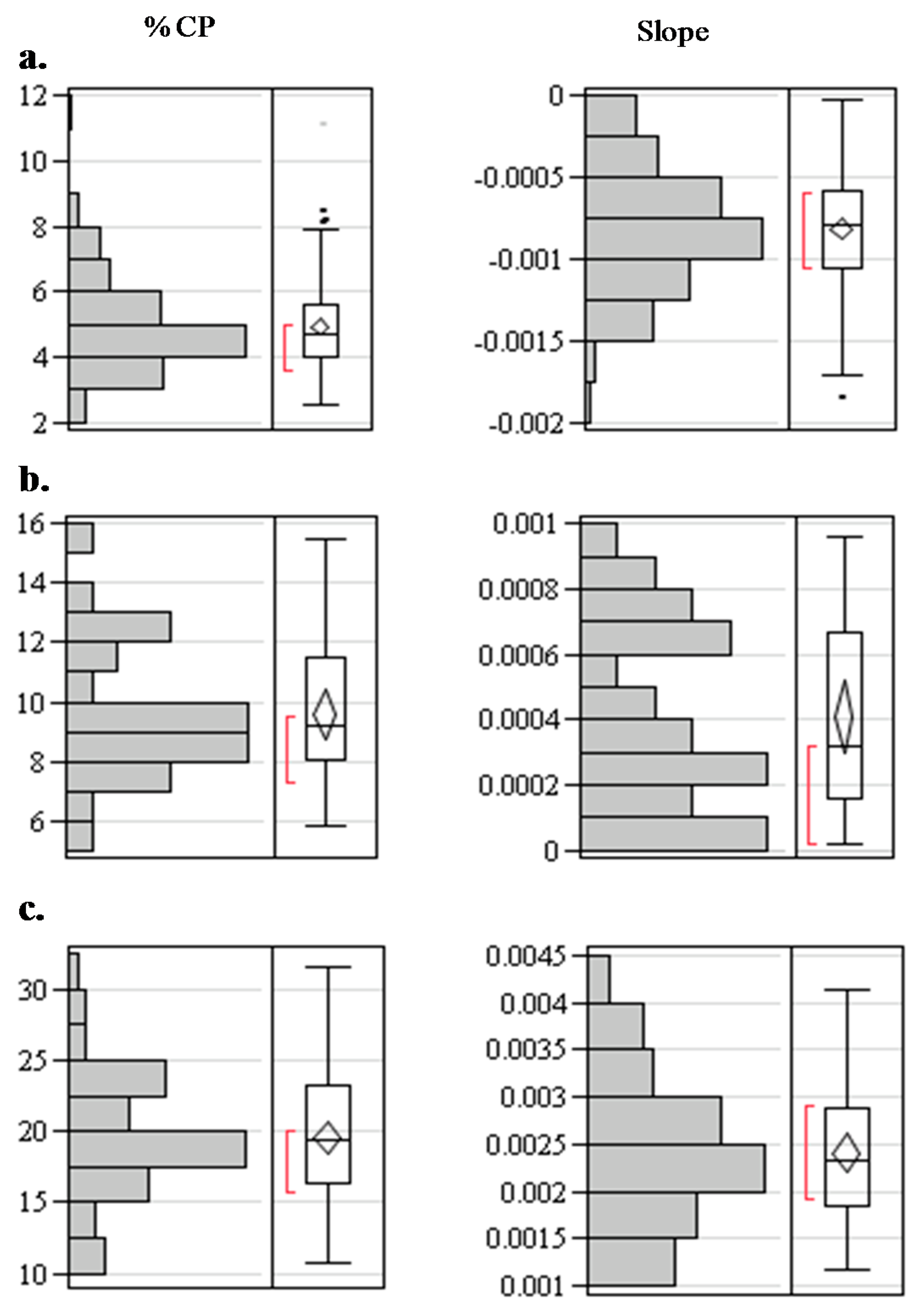
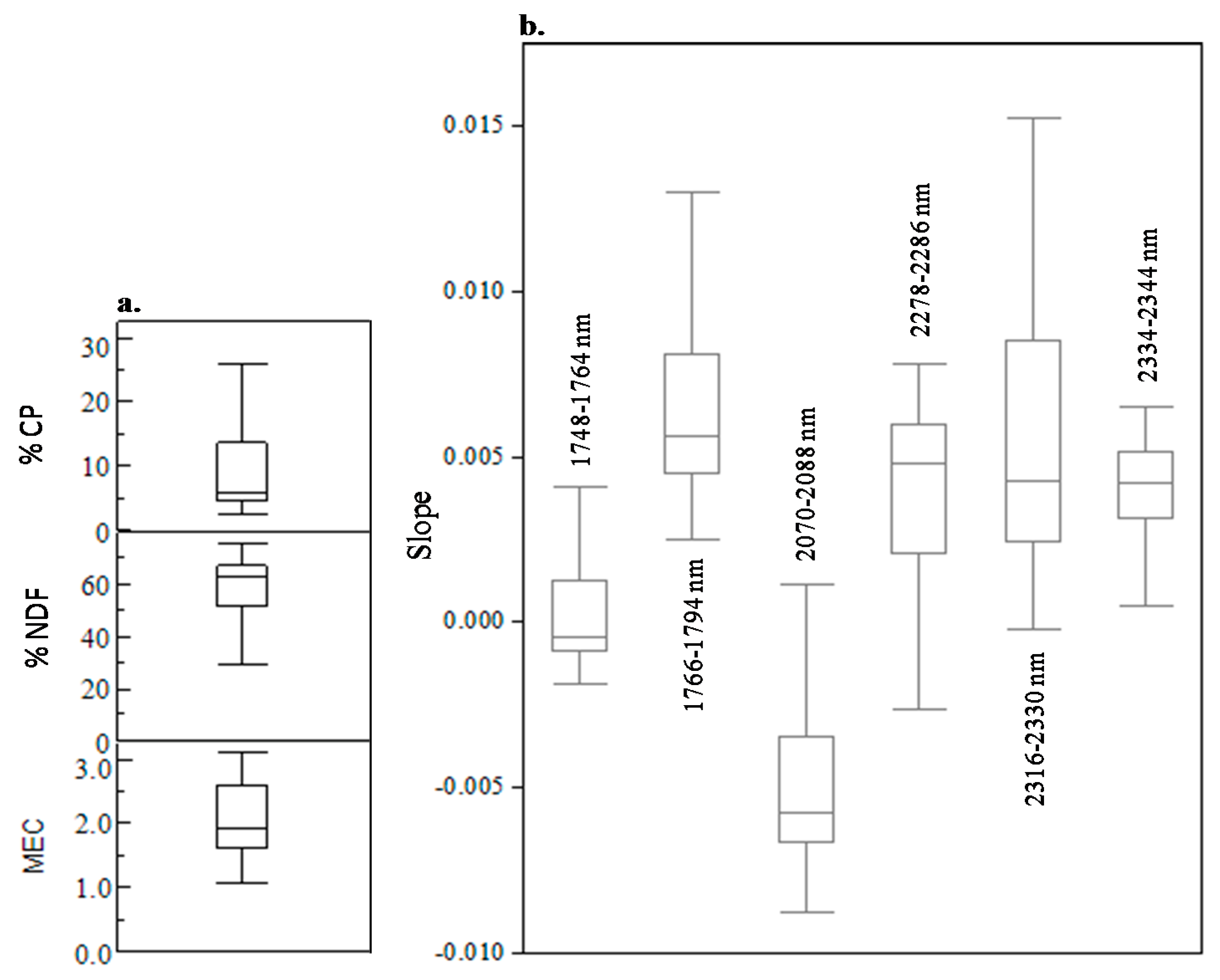
3.1. Chemical Reference: CP, NDF, MEC
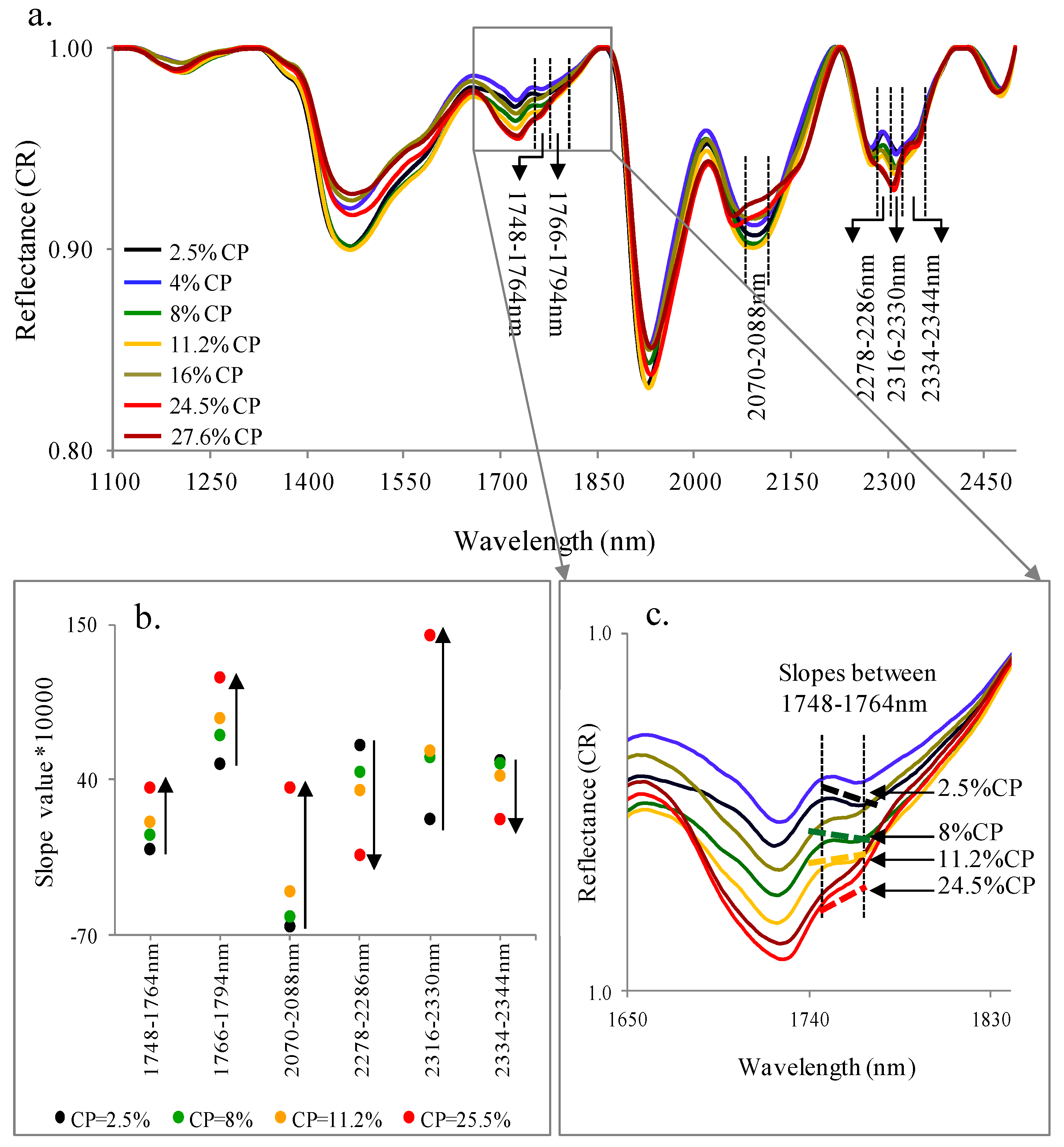
3.2. Spectral Slope Analyses


| %CP | |||
| Spectral Range | Low (≤4.5%) | Medium (4.5%–13%) | High (≥13%) |
| 1748–1764 nm | Slope ≤ −0.0008 | −0.0008 < Slope< 0.001 | Slope ≥ 0.001 |
| 1766–1794 nm | Slope ≤ 0.005 | 0.005 < Slope< 0.008 | Slope ≥ 0.008 |
| 2070–2088 nm | Slope ≤ −0.0065 | −0.0065 < Slope< –0.003 | Slope ≥ −0.003 |
| 2278–2286 nm | Slope ≥ 0.0058 | 0.0025 < Slope < 0.0058 | Slope ≤ 0.0025 |
| 2316–2330 nm | Slope ≤ 0.003 | 0.003 < Slope < 0.008 | Slope ≥ 0.008 |
| 2334–2344 nm | Slope ≥ 0.0048 | 0.0034 < Slope < 0.0048 | Slope ≤ 0.0034 |
| %NDF | |||
| Spectral Range | Low (≥67%) | Medium (53%–67%) | High (≤53%) |
| 1748–1764 nm | Slope ≤ −0.0008 | −0.0008 < Slope < 0.001 | Slope ≥0.001 |
| 1766–1794 nm | Slope ≤ 0.0052 | 0.0052 < Slope < 0.0076 | Slope ≥ 0.0076 |
| 2070–2088 nm | Slope ≤ −0.0065 | −0.0065 < Slope < −0.0032 | Slope ≥ −0.0032 |
| 2278–2286 nm | Slope ≥ 0.0058 | 0.0026 < Slope < 0.0058 | Slope ≤ 0.0026 |
| 2316–2330 nm | Slope ≤ 0.0032 | 0.0076 > Slope > 0.0032 | Slope ≥ 0.0076 |
| 2334–2344 nm | Slope ≥ 0.005 | 0.005 > Slope > 0.0033 | Slope ≤ 0.0033 |
| MEC | |||
| Spectral Range | Low (≤1.6) | Medium (1.6–2.5) | High (≥2.5) |
| 1748–1764 nm | Slope ≤ −0.0005 | −0.0005 < Slope < 0.0016 | Slope ≥ 0.0016 |
| 1766–1794 nm | Slope ≤ 0.0053 | 0.0053 < Slope < 0.0091 | Slope ≥ 0.0091 |
| 2070–2088 nm | Slope ≤ −0.0062 | −0.0062 < Slope < −0.0022 | Slope ≥ −0.0022 |
| 2278–2286 nm | Slope ≥ 0.0057 | 0.0018 < Slope < 0.0057 | Slope ≤ 0.0018 |
| 2316–2330 nm | Slope ≤ 0.003 | 0.003 < Slope < 0.0093 | Slope ≥ 0.0093 |
| 2334–2344 nm | Slope ≥ 0.0048 | 0.0031 < Slope < 0.0048 | Slope ≤ 0.0031 |
| % CP | Total Per Category Based on Chemical Data | Total Per Category Based on Slope Algorithm | |||||||||||
|---|---|---|---|---|---|---|---|---|---|---|---|---|---|
| 1748–1764 nm | 1764–1794 nm | 2070–2088 nm | 2278–2286 nm | 2316–2330 nm | 2334–2344 nm | ||||||||
| Low (≤4.5%) | 54 | 41 | 76% | 39 | 72% | 41 | 76% | 41 | 76% | 43 | 80% | 43 | 80% |
| Medium (4.5%–13%) | 114 | 83 | 73% | 57 | 50% | 84 | 74% | 79 | 69% | 72 | 63% | 68 | 60% |
| High (≥13%) | 57 | 55 | 96% | 48 | 84% | 49 | 86% | 56 | 98% | 55 | 96% | 49 | 86% |
| Total | 225 | 179 | 80% | 144 | 64% | 174 | 77% | 176 | 78% | 170 | 76% | 160 | 71% |
| % NDF | |||||||||||||
| Low (≥67%) | 64 | 49 | 77% | 49 | 77% | 44 | 69% | 48 | 75% | 46 | 72% | 45 | 70% |
| Medium (53%–67%) | 109 | 79 | 72% | 40 | 37% | 72 | 66% | 71 | 65% | 57 | 52% | 64 | 59% |
| High (≤53%) | 62 | 54 | 87% | 51 | 82% | 49 | 79% | 56 | 90% | 58 | 94% | 50 | 81% |
| Total | 235 | 182 | 77% | 140 | 60% | 165 | 70% | 175 | 74% | 161 | 69% | 159 | 68% |
| MEC | |||||||||||||
| Low (≤1.6) | 39 | 30 | 77% | 26 | 67% | 25 | 64% | 30 | 77% | 34 | 87% | 22 | 56% |
| Medium (1.6%–2.5) | 80 | 44 | 55% | 41 | 51% | 42 | 53% | 48 | 60% | 47 | 59% | 37 | 46% |
| High (≥2.5) | 47 | 42 | 89% | 41 | 87% | 41 | 87% | 40 | 85% | 41 | 87% | 37 | 79% |
| Total | 166 | 116 | 70% | 108 | 65% | 108 | 65% | 118 | 71% | 122 | 73% | 96 | 58% |
| % CP | |||
| Spectral Range | Low (≤4.5%) | Medium (4.5%–13%) | High (≥13%) |
| 1747–1770nm | Slope ≤ 0.00025 | 0.00025 < Slope< 0.003 | Slope ≥ 0.003 |
| 2061–2096 nm | Slope ≤ −0.014 | −0.014 < Slope< −0.008 | Slope ≥ −0.008 |
| 2270–2293 nm | Slope ≥ 0.01 | 0.01 > Slope> 0.0045 | Slope ≤ 0.0045 |
| 2306–2317 nm | Slope ≤ −0.001 | −0.001 < Slope< 0.0025 | Slope ≥ 0.0025 |
| 2317–2328 nm | Slope ≤ 0.0045 | 0.0045 < Slope < 0.008 | Slope ≥ 0.008 |
| % NDF | |||
| Spectral Range | Low (≥67%) | Medium (53%–67%) | High (≤53%) |
| 1747–1770nm | Slope ≤ 0.0005 | 0.0005 < Slope< 0.003 | Slope ≥ 0.003 |
| 2061–2096 nm | Slope ≤ −0.014 | −0.014 < Slope< −0.008 | Slope ≥ −0.008 |
| 2270–2293 nm | Slope ≥ 0.01 | 0.01 > Slope> 0.0035 | Slope ≤ 0.0035 |
| 2306–2317 nm | Slope ≤ 0.0004 | 0.0004 < Slope< 0.003 | Slope ≥ 0.003 |
| 2317–2328 nm | Slope ≤ 0.0045 | 0.0045 < Slope < 0.008 | Slope ≥ 0.008 |
| MEC | |||
| Spectral Range | Low (≤1) | Medium (1.6–2.5) | High (≥2.5) |
| 1747–1770nm | Slope ≤ 0.001 | 0.001 < Slope< 0.004 | Slope ≥ 0.004 |
| 2061–2096 nm | Slope ≤ −0.013 | −0.013 < Slope< −0.006 | Slope ≥ −0.006 |
| 2270–2293 nm | Slope ≥ 0.01 | 0.01 > Slope> 0.001 | Slope ≤ 0.001 |
| 2306–2317 nm | Slope ≤ −0.0005 | −0.0005 < Slope< 0.0035 | Slope ≥ 0.0035 |
| 2317–2328 nm | Slope ≤ 0.0045 | 0.0045 < Slope < 0.009 | Slope ≥ 0.009 |
| % CP | Total Per Category Based on Chemical Data | Total Per Category Based on Slope Algorithm | |||||||||
|---|---|---|---|---|---|---|---|---|---|---|---|
| 1747–1770 nm | 2061–2096 nm | 2270–2293 nm | 2306–2317 nm | 2317–2328 nm | |||||||
| Low (≤4.5%) | 54 | 48 | 89% | 38 | 70% | 45 | 83% | 49 | 91% | 46 | 85% |
| Medium (4.5%–13%) | 114 | 72 | 63% | 80 | 70% | 66 | 58% | 77 | 68% | 66 | 58% |
| High (≥13%) | 57 | 55 | 96% | 49 | 86% | 57 | 100% | 55 | 96% | 55 | 96% |
| Total | 225 | 175 | 78% | 167 | 74% | 168 | 75% | 181 | 80% | 167 | 74% |
| % NDF | |||||||||||
| Low (≥67%) | 64 | 42 | 66% | 41 | 64% | 51 | 80% | 61 | 95% | 46 | 72% |
| Medium (53%–67%) | 109 | 73 | 67% | 63 | 58% | 63 | 58% | 36 | 33% | 57 | 52% |
| High (≤53%) | 62 | 49 | 79% | 49 | 79% | 56 | 90% | 53 | 85% | 57 | 92% |
| Total | 235 | 164 | 70% | 153 | 65% | 170 | 72% | 150 | 64% | 160 | 68% |
| MEC | |||||||||||
| Low (≤1.6) | 39 | 33 | 85% | 26 | 67% | 28 | 72% | 29 | 74% | 33 | 85% |
| Medium (1.6–2.5) | 80 | 39 | 49% | 37 | 46% | 50 | 63% | 40 | 50% | 45 | 56% |
| High (≥2.5) | 47 | 44 | 94% | 39 | 83% | 44 | 94% | 42 | 89% | 42 | 89% |
| Total | 166 | 116 | 70% | 102 | 61% | 122 | 73% | 111 | 67% | 120 | 72% |
3.3. PLS Analyses

| Spectral Range (nm) (Number of Bands) | CP Model’s Statistical Characteristics | CP Best Model | NDF Model’s Statistical Characteristics | NDF Best Model | MEC Model’s Statistical Characteristics | MEC Best Model | ||||
|---|---|---|---|---|---|---|---|---|---|---|
| Prediction | Validation | Prediction | Validation | Prediction | Validation | |||||
| 1748–1764 (n = 9) | Slope: | 0.934 | 0.933 | 2 | 0.856 | 0.850 | 4 | 0.789 | 0.792 | 5 |
| Offset: | 0.6 | 0.606 | 8.508 | 8.874 | 0.429 | 0.423 | ||||
| RMSE: | 1.703 | 1.757 | 4.183 | 4.305 | 0.252 | 0.263 | ||||
| R2: | 0.934 | 0.931 | 0.856 | 0.848 | 0.789 | 0.769 | ||||
| 1766–1794 (n = 15) | Slope: | 0.913 | 0.908 | 3 | 0.797 | 0.785 | 5 | 0.794 | 0.782 | 4 |
| Offset: | 0.79 | 0.834 | 12.045 | 12.750 | 0.418 | 0.445 | ||||
| RMSE: | 1.954 | 2.02 | 4.977 | 5.098 | 0.248 | 0.259 | ||||
| R2: | 0.913 | 0.909 | 0.797 | 0.792 | 0.794 | 0.783 | ||||
| 2070–2088 (n = 10) | Slope: | 0.897 | 0.899 | 5 | 0.865 | 0.859 | 2 | 0.716 | 0.700 | 7 |
| Offset: | 0.932 | 0.912 | 8.019 | 8.345 | 0.576 | 0.623 | ||||
| RMSE: | 2.122 | 2.204 | 4.062 | 4.133 | 0.291 | 0.324 | ||||
| R2: | 0.897 | 0.891 | 0.865 | 0.861 | 0.716 | 0.654 | ||||
| 2278–2286 (n = 4) | Slope: | 0.903 | 0.898 | 4 | 0.856 | 0.854 | 3 | 0.805 | 0.796 | 3 |
| Offset: | 0.871 | 0.9 | 8.499 | 8.677 | 0.395 | 0.419 | ||||
| RMSE: | 2.051 | 2.096 | 4.181 | 4.217 | 0.241 | 0.251 | ||||
| R2: | 0.904 | 0.902 | 0.856 | 0.855 | 0.805 | 0.795 | ||||
| 2316–2330 (n = 8) | Slope: | 0.892 | 0.889 | 6 | 0.782 | 0.761 | 7 | 0.812 | 0.802 | 2 |
| Offset: | 0.978 | 1.004 | 12.911 | 14.157 | 0.380 | 0.406 | ||||
| RMSE: | 2.173 | 2.215 | 5.153 | 5.420 | 0.237 | 0.243 | ||||
| R2: | 0.891 | 0.888 | 0.782 | 0.760 | 0.812 | 0.804 | ||||
| 2334–2344 (n = 6) | Slope: | 0.78 | 0.77 | 7 | 0.787 | 0.785 | 6 | 0.715 | 0.707 | 6 |
| Offset: | 1.987 | 2.05 | 12.629 | 12.736 | 0.579 | 0.594 | ||||
| RMSE: | 3.09 | 3.17 | 5.097 | 5.219 | 0.292 | 0.302 | ||||
| R2: | 0.78 | 0.77 | 0.787 | 0.778 | 0.715 | 0.703 | ||||
| All ranges (n = 53) | Slope: | 0.967 | 0.956 | 1 | 0.893 | 0.882 | 1 | 0.832 | 0.823 | 1 |
| Offset: | 0.32 | 0.39 | 6.310 | 6.850 | 0.340 | 0.368 | ||||
| RMSE: | 1.246 | 1.355 | 3.604 | 3.858 | 0.224 | 0.241 | ||||
| R2: | 0.964 | 0.958 | 0.893 | 0.878 | 0.833 | 0.809 | ||||
4. Conclusions
Acknowledgments
Author Contributions
Conflicts of Interest
References
- Svoray, T.; Perevolotsky, A.; Atkinson, P.M. Ecological sustainability in rangelands: The contribution of remote sensing. Int. J. Remote Sens. 2013, 34, 6216–6242. [Google Scholar] [CrossRef]
- Association of Official Analytical Chemists (AOAC). Official Methods of Analysis, 15th ed.; AOAC: Washington, DC, USA, 1990. [Google Scholar]
- Association of Official Analytical Chemists (AOAC), International. Official Methods of Analysis, 16th ed.; AOAC: Arlington, VA, USA, 1995. [Google Scholar]
- Goering, H.K.; van Soest, P.J. Forage fiber analysis (apparatus, reagents, procedures and some applications). In Agriculture Handbook; No. 379; Agriculture Research Service, United States Department of Agriculture: Washington, DC, USA, 1970. [Google Scholar]
- Blanco, M.; Villarroya, I. NIR spectroscopy: A rapid-response analytical tool. Trends Anal. Chem. 2002, 21, 240–250. [Google Scholar] [CrossRef]
- Dematte, J.A.M.; Campos, R.C.; Alves, M.C.; Fiorio, P.R.; Nanni, M.R. Visible-NIR reflectance: A new approach on soil evaluation. Geoderma 2004, 12, 95–112. [Google Scholar] [CrossRef]
- Goldshleger, N.; Chudnovsky, A.; Ben-Binyamin, R. Predicting salinity in tomatoes using soil reflectance spectra. Int. J. Remote Sens. 2013, 34, 6079–6093. [Google Scholar] [CrossRef]
- Landau, S.; Glasser, T.; Dvash, L. Monitoring nutrition in small ruminants by aids of near infrared spectroscopy (NIRS) technology: A review. Small Rumin. Res. 2006, 61, 1–11. [Google Scholar] [CrossRef]
- Norris, K.H.; Barners, R.F.; Moore, J.E.; Shenk, J.S. Predicting forage quality by infrared reflectance spectroscopy. J. Anim. Sci. 1976, 43, 889–897. [Google Scholar]
- Ben-Dor, E.; Banin, A. Near-infrared analysis as a method to simultaneously evaluate several soil properties. Soil Sci. Soc. Am. J. 1995, 59, 364–372. [Google Scholar] [CrossRef]
- Ben-Dor, E.; Inbar, Y.; Chen, Y. The reflectance spectra of organic matter in the visible near-infrared and short wave infrared region (400–2500 nm) during a controlled decomposition process. Remote Sens. Environ. 1997, 61, 1–15. [Google Scholar] [CrossRef]
- Chabrillat, S.; Ben-Dor, E.; Viscarra Rossel, R.A.; Demattê, J.A.M. Quantitative soil spectroscopy. Appl. Environ. Soil Sci. 2013. [Google Scholar] [CrossRef]
- Chudnovsky, A.; Ben-Dor, E.; Paz, E. Using NIRS for rapid assessment of sediment dust in the indoor environment. J. Near Infrared Spectrosc. 2007, 15, 59–70. [Google Scholar] [CrossRef]
- Karnieli, A. Development and implementation of spectral crust index over dune sands. Int. J. Remote Sens. 1997, 18, 1207–1220. [Google Scholar] [CrossRef]
- Karnieli, A.; Kidron, G.J.; Glaesser, C.; Ben-Dor, E. Spectral characteristics of cyanobacteria soil crust in semiarid environments. Remote Sens. Environ. 1999, 69, 67–75. [Google Scholar] [CrossRef]
- Kooistra, L.; Wehrens, R.; Leuven, W.; Buydens, L. Possibilities of visible-near-infrared spectroscopy for the assessment of soil contamination in river floodplains. Anal. Chim. Acta 2001, 446, 97–105. [Google Scholar] [CrossRef]
- Kooistra, L.; Wanders, G.; Epemac, R.; Leuven, W.; Wehrens, L.; Buydens, L. The potential of field spectroscopy for the assessment of sediment properties in river floodplains. Anal. Chim. Acta 2003, 484, 189–200. [Google Scholar] [CrossRef]
- Shoshany, M.; Svoray, T.; Curran, P.J.; Foody, G.M.; Perevolotsky, A. The relationship between ERS-2 SAR backscatter and soil moisture: Generalization from a humid to semi-arid transect. Int. J. Remote Sens. 2000, 21, 2337–2343. [Google Scholar] [CrossRef]
- Viscarra-Rossel, R.A.; Walvoort, D.J.J.; McBratney, A.B.; Janik, L.J.; Skjemstad, J.O. Visible, near infrared, mid infrared or combined diffuse reflectance spectroscopy for simultaneous assessment of various soil properties. Geoderma 2006, 131, 59–75. [Google Scholar] [CrossRef]
- Curran, P.J. Remote sensing of foliar chemistry. Remote Sens. Environ. 1989, 30, 271–278. [Google Scholar] [CrossRef]
- Murray, I.; Williams, P.C. Chemical principles of near infrared technology. In Near Infrared Technology in Agriculture and Food Industries; Wiliams, P.C., Noriss, K.H., Eds.; American Association of Cereal Chemistry Inc.: St. Paul, MN, USA, 1987; pp. 17–31. [Google Scholar]
- Workman, J., Jr.; Weyer, L. Practical Guide to Interpretive Near-Infrared Spectroscopy; CRC Press/Taylor & Francis Group: Boca Raton, FL, USA, 2008. [Google Scholar]
- Baumgardner, M.F.; Silva, L.F.; Biehl, L.L.; Stoner, E.R. Reflectance properties of soils. Adv. Agron. 1985, 38, 1–44. [Google Scholar]
- Dalal, R.C.; Henry, R.J. Simultaneous determination of moisture, organic carbon and total nitrogen by near infrared reflectance spectroscopy. Soil Sci. Soc. Am. J. 1986, 50, 120–123. [Google Scholar] [CrossRef]
- Schwanninger, M.; Rodrigues, J.C.; Fackler, K. A review of band assignments in near infrared spectra of wood and wood components. J. Near Infrared Spectrosc. 2011, 19, 287–308. [Google Scholar] [CrossRef]
- Decruyenaere, V.; Lecomte, P.; Demarquilly, C.; Aufrere, J.; Dardenne, P.; Stilmant, D.; Buldgen, A. Evaluation of green forage intake and digestibility in ruminants using near infrared reflectance spectroscopy (NIRS): Developing a global calibration. Anim. Feed Sci. Technol. 2009, 148, 138–156. [Google Scholar] [CrossRef]
- Givens, D.I.; de Boever, J.L.; Deaville, E.R. The principles, practices and some future applications of near infrared spectroscopy for predicting the nutritive value of foods for animals and humans. Nutr. Res. Rev. 1997, 10, 83–114. [Google Scholar] [CrossRef] [PubMed]
- Schellberg, J.; Hill, M.J.; Gerhards, R.; Rothmund, M.; Braun, M. Precision agriculture on grassland: Applications, perspectives and constraints. Eur. J. Agron. 2008, 29, 59–71. [Google Scholar] [CrossRef]
- Pullanagari, R.; Yule, I.; Tuohy, M.; Hedley, M.; Dynes, R.; King, W. In-field hyperspectral proximal sensing for estimating quality parameters of mixed pasture. Precis. Agric. 2012, 13, 351–369. [Google Scholar] [CrossRef]
- Pullanagari, R.; Yule, I.; Tuohy, M.; Hedley, M.; Dynes, R.; King, W. Multi-spectral radiometry to estimate pasture quality components. Precis. Agric. 2012, 13, 442–456. [Google Scholar] [CrossRef]
- Sanches, D.; Tuohy, M.P.; Hedley, M.J.; Bretherton, M.R. Large, durable and low-cost reflectance standard for field remote sensing applications. Int. J. Remote Sens. 2009, 30, 2309–2319. [Google Scholar] [CrossRef]
- Mutanga, O.; Skidmore, A.K. Narrow band vegetation indices overcome the saturation problem in biomass estimation. Int. J. Remote Sens. 2004, 25, 3999–4014. [Google Scholar] [CrossRef]
- Mutanga, O.; Skidmore, A.K. Integrating imaging spectroscopy and neural networks to map grass quality in the Kruger National Park, South Africa. Remote Sens. Environ. 2004, 90, 104–115. [Google Scholar] [CrossRef]
- Pimstein, A.; Karnieli, A.; Bansal, S.K.; Bonfil, D. Exploring remotely sensed technologies for monitoring wheat potassium and phosphorus using field spectroscopy. Field Crops Res. 2011, 121, 125–135. [Google Scholar] [CrossRef]
- Mutanga, O.; Skidmore, A.K.; Prins, H.H.T. Predicting in situ pasture quality in the Kruger National Park, South Africa, using continuum-removed absorption features. Remote Sens. Environ. 2004, 89, 393–408. [Google Scholar] [CrossRef]
- Lehnert, L.W.; Meyer, H.; Meyer, N.; Reudenbach, C.; Bendix, J. A hyperspectral indicator system for rangeland degradation on the Tibetan Plateau: A case study towards spaceborne monitoring. Ecol. Indic. 2014, 39, 54–64. [Google Scholar] [CrossRef]
- Kawamura, K.; Watanabe, N.; Sakanoue, S.; Yoshitoshi, R.; Odagawa, S. Herbage biomass and quality status assessment in a mixed sown pasture from airborne based hyperspectral imaging. In Proceedings of the 33rd Asian Conference on Remote Sensing, Pattaya, Thailand, 26–30 November 2012; pp. 2220–2228.
- Stern, A.; Gradus, Y.; Meir, A.; Krakover, S.; Tsoar, H. Atlas of the Negev; Ben Gurion University of the Negev: Beer-Sheva, Israel, 1986. [Google Scholar]
- The Israel Meteorological Service. Available online: http://www.ims.gov.il/IMSEng/ (accessed on 22 December 2014).
- Dan, J.; Yaalon, D.; Kundzimzinsky, H.; Raz, Z. The Soil of Israel; ARO Publication Bulletin No. 168 (in Hebrew). Volcani Center: Bet-Dagan, Israel, 1977. [Google Scholar]
- Zaady, E.; Levacov, R.; Shachak, M. Application of the herbicide, Simazine, and its effect on soil surface parameters and vegetation in a patchy desert landscape. Arid Land Res. Manag. 2004, 18, 397–410. [Google Scholar] [CrossRef]
- Feinbrun-Dothan, N.; Danin, A. Analytical Flora of Eretz-Israel; Cana Publishers: Jerusalem, Israel, 1991. [Google Scholar]
- Zaady, E.; Yonatan, R.; Shachak, M.; Perevolotsky, A. The effects of grazing on abiotic and biotic parameters in a semiarid ecosystem: A case study from the northern Negev desert, Israel. Arid Land Res. Manag. 2001, 15, 245–261. [Google Scholar] [CrossRef]
- Henkin, Z.; Landau, S.; Ungar, E.D.; Perevolotsky, A.; Yehuda, Y.; Sternberg, M. Effect of timing and intensity of grazing on the herbage quality of a Mediterranean rangeland. J. Anim. Feed Sci. 2007, 16, 318–322. [Google Scholar]
- Henkin, Z.; Ungar, E.D.; Dvash, L.; Perevolotsky, A.; Yehuda, Y.; Sternberg, M.; Voet, H.; Landau, S.Y. Effects of cattle grazing on herbage quality in a herbaceous Mediterranean rangeland. Grass Forage Sci. 2011, 66, 516–525. [Google Scholar] [CrossRef]
- Landau, S.; Friedman, S.; Brenner, S.; Bruckental, I.; Weinberg, Z.G.; Ashbell, G.; Hen, Y.; Dvash, L.; Leshem, Y. The value of safflower (Carthamus tinctorius) hay and silage grown under Mediterranean conditions as forage for dairy cattle. Livest. Prod. Sci. 2004, 88, 263–271. [Google Scholar] [CrossRef]
- Landau, S.; Giger-Reverdin, S.; Rapetti, L.; Dvash, L.; Dorleans, M.; Ungar, E.D. Data mining old digestibility trials for nutritional monitoring in confined goats with aids of fecal near infra-red spectrometry. Small Ruminant Res. 2008, 77, 146–158. [Google Scholar] [CrossRef]
- Tilley, J.M.A.; Terry, R.A. A two-stage technique for the in vitro digestion of forage crops. J. Br. Grassl. Soc. 1963, 18, 104–111. [Google Scholar] [CrossRef]
- Wagner, J.J.; Lusby, K.S.; Oltjen, J.W.; Rakestraw, J.; Wettemann, R.P.; Walters, L.E. Carcass composition in mature Hereford cows: Estimation and effect on daily metabolizable energy requirement during winter. J. Anim. Sci. 1988, 66, 603–612. [Google Scholar] [PubMed]
- Cook, C.W.; Stoddart, L.A.; Harris, L.E. Determining the digestibility and metabolizable energy of winter range plants by sheep. J. Anim. Sci. 1952, 11, 578–590. [Google Scholar]
- Noomen, M.F.; Skidmore, A.K.; van der Meer, F.D.; Prins, H.H.T. Continuum removed band depth analysis for detecting the effects of natural gas, methane and ethane on maize reflectance. Remote Sens. Environ. 2006, 105, 262–270. [Google Scholar] [CrossRef]
- Curcio, D.; Ciraolo, G.; D’Asaro, F.; Minacapilli, M. Prediction of soil texture distributions using VNIR-SWIR reflectance rpectroscopy. Procedia Environ. Sci. 2013, 19, 494–503. [Google Scholar] [CrossRef]
- Clark, R.N. Spectroscopy of rocks and minerals and principle of spectroscopy. In Manual of Remote Sensing; Rencz, A.N., Ed.; John Wiley & Sons: New York, NY, USA, 1999; pp. 3–59. [Google Scholar]
- SPECIM, Spectral Imaging Ltd. Available online: http://www.specim.fi (accessed on 22 December 2014).
- Esbensen, K. Multivariate data analyses. In Practice—An Introduction to Multivariate Data Analyses and Experimental Design; Aalborg University, CAMO: Esbjerg, Denmark, 2002. [Google Scholar]
- Wold, S.; Sjostrom, M.; Eriksson, L. PLS-regression: A basic tool of chemometrics. Chemom. Intell. Lab. Syst. 2001, 58, 109–130. [Google Scholar] [CrossRef]
- Øvergaard, S.I.; Isaksson, T.; Korsaeth, A. Prediction of wheat yield and protein using remote sensors on plots—Part I: Assessing near infrared model robustness for year and site variations. J. Near Infrared Spectrosc. 2013, 21, 117–131. [Google Scholar] [CrossRef]
- Pullanagari, R. Proximal Sensing Techniques to Monitor Pasture Quality and Quantity on Dairy Farms. Ph.D. Thesis, Massey University, Manawatu, New Zealand, 2011. [Google Scholar]
- Landau, S.; Nitzan, R.; Barkai, D.; Dvash, L. Excretal near infrared reflectance spectrometry to monitor the nutrient content of diets of grazing young ostriches (Struthio camelus). S. Afr. J. Anim. Sci. 2006, 36, 248–256. [Google Scholar]
- Swart, E.; Brand, T.S.; Engelbrecht, J. The use of near infrared spectroscopy (NIRS) to predict the chemical composition of feed samples used in ostrich total mixed ration. S. Afr. J. Anim. Sci. 2012, 42, 550–554. [Google Scholar]
- Ben-Dor, E.; Taylor, R.G.; Hill, J.; Dematte, J.A.M.; Whiting, M.L.; Chabrillat, S.; Sommer, S. Imaging spectrometry for soil applications. In Advances in Agronomy; Sparks, D.L., Ed.; Elsevier Inc.: Newark, DE, USA, 2008; Volume 97, pp. 321–392. [Google Scholar]
© 2014 by the authors; licensee MDPI, Basel, Switzerland. This article is an open access article distributed under the terms and conditions of the Creative Commons Attribution license (http://creativecommons.org/licenses/by/4.0/).
Share and Cite
Lugassi, R.; Chudnovsky, A.; Zaady, E.; Dvash, L.; Goldshleger, N. Spectral Slope as an Indicator of Pasture Quality. Remote Sens. 2015, 7, 256-274. https://doi.org/10.3390/rs70100256
Lugassi R, Chudnovsky A, Zaady E, Dvash L, Goldshleger N. Spectral Slope as an Indicator of Pasture Quality. Remote Sensing. 2015; 7(1):256-274. https://doi.org/10.3390/rs70100256
Chicago/Turabian StyleLugassi, Rachel, Alexandra Chudnovsky, Eli Zaady, Levana Dvash, and Naftaly Goldshleger. 2015. "Spectral Slope as an Indicator of Pasture Quality" Remote Sensing 7, no. 1: 256-274. https://doi.org/10.3390/rs70100256
APA StyleLugassi, R., Chudnovsky, A., Zaady, E., Dvash, L., & Goldshleger, N. (2015). Spectral Slope as an Indicator of Pasture Quality. Remote Sensing, 7(1), 256-274. https://doi.org/10.3390/rs70100256