Mapping Levees Using LiDAR Data and Multispectral Orthoimages in the Nakdong River Basins, South Korea

Abstract
: Mapping levees is important for analyzing levee surfaces, assessing levee stability, etc. Historically, mapping levees has been carried out using ground surveying methods or only one type of remote sensing dataset. This research aims to map levees using airborne topographic LiDAR data and multispectral orthoimages taken in the Nakdong River Basins. Levee surfaces consist of multiple objects with different geometric and spectral patterns. This research investigates different methods for identifying multiple levee components, such as major objects and eroded areas. Multiple geometric analysis approaches such as the slope classification method, and elevation and area analysis are used to identify the levee crown, berm, slope surfaces, and the eroded area, with different geometric patterns using the LiDAR data. Next, a spectral analysis approach, such as the clustering algorithm, is used to identify the major objects with different spectral patterns on the identified components using multispectral orthoimages. Finally, multiple levee components, including major objects and eroded areas, are identified. The accuracy of the results shows that the various components on the levee surfaces are well identified using the proposed methodology. The obtained results are applied for evaluating the physical condition of the levees in the study area.
1. Introduction
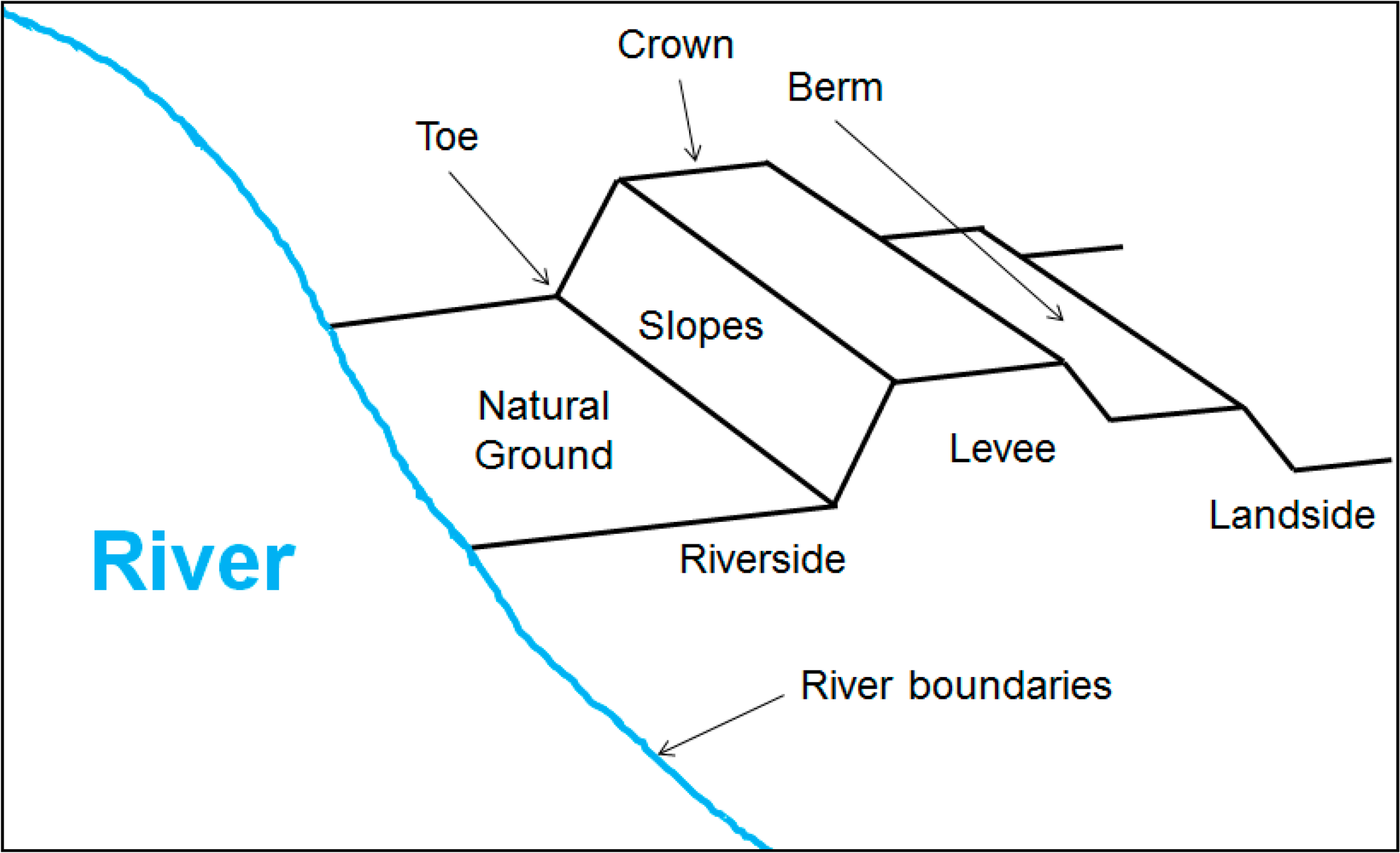
A levee is defined as “a man-made structure; usually an earthen embankment, designed and constructed in accordance with sound engineering practices to contain, control or divert the flow of water to provide protection from temporary flooding” [1]. The elements that constitute a typical levee are illustrated in Figure 1.
As can be seen in Figure 1, the levee crown is defined as “the flat surface at the top of a levee that is equal to or narrower than the base”, and the levee toe is defined as “the edge of the levee where the base meets the natural ground” [1]. The levee berm is a man-made mound located between the levee toe and crown; it has generally been used as a trail road for human activities and vehicles [2]. The width and height of the levee berm are primarily dependent on the ground conditions, levee heights, and the amount of available land [2,3].
Levees are generally covered by various materials, such as the asphalt or gravel road on the crown surface and concrete or vegetation on the slope surfaces. Multiple factors, such as the objectives of levee construction, local geological conditions, flooding risk factors, and local weather conditions, affect the type of materials selected to cover a levee’s surface. In general, levees constructed in areas of high-value properties are designed to have relatively steep slopes, while levees constructed in areas of low-value properties are designed to have gentle slopes [3]. Additionally, the riverside slope surfaces of levees are generally designed with their surfaces covered by concrete or stone blocks because their function is to protect the urban areas built along a river’s course, or because the surfaces of such levees are considered to be at risk from wave actions [2,3].
Earthen levees are designed, constructed and maintained by local, state, or federal bodies. In the United States, the United States Army Corps of Engineers (USACE) provides a manual that presents the basic principles used in the design and construction of levees and levee systems [3]. USACE also provides the levee safety program to assess the 2500 nationwide levee systems in the U.S. [4]. In South Korea, the Ministry of Land, Infrastructure, and Transport (MOLIT) provides a manual to present the basic principles for the design and construction of levees and levee systems [5]. The Water Management Information System (WAMIS) website provides information about the levee systems in South Korea, such as the lengths of the systems, the major materials covering the levee surfaces, the locations of the systems, the average slope degrees of the systems, and the expected maximum water elevations [6].
Historically, research on the detection of the specific features on levee surfaces has been carried out using one type of remote sensing dataset. Bishop et al. [7] extracted the levee crown from laser radar data using the least-cost path method and the flip 7 filter. Hossain et al. [8] detected levee slides from IKONOS and Quickbird imagery using the Iterative Self-Organizing Data Analysis Technique (ISODATA) clustering. Mahrooghy et al. [9] detected levee slides from the terrasar-x data. Hossain and Easson [10] detected levee slides from the hyperspectral images using the vegetation indices.
The use of a single data set is limited for mapping levees due to the following reasons: Levees consist of various components such as the crown, slope, and berm surfaces with different geometric patterns, and multiple objects such as an asphalt or gravel road, concrete, and vegetation or soil with different spectral patterns. In addition, the eroded areas, randomly located on the levee surfaces, have geometric patterns different from the other objects on levee surfaces. Hence, the use of the multiple data sets is necessary for identifying the multiple objects on levee surfaces with different geometric and spectral patterns. In this research, multiple methods for identifying the multiple major objects and the eroded areas on the levees using the geometric information obtained from the LiDAR data and the spectral information obtained from the multispectral orthoimages are proposed.
2. Study Area and Data Sets
The study area for this research is a river basin in a 22 kilometer stretch of Nakdong River, which passes through the South Korean cities of Changnyeong, Milyang and Changwon. Eight levees are located in the study area (Figure 2).
The Nakdong River is the longest river in South Korea with a total length of 525 km. The annual rainfall in the study area is 1229.0 mm [5].
The levees in the study area were designed to have the minimum height 13.5 m and the minimum crown widths 4 m [6]. All levees in the study area are typical levees, and their surfaces are generally covered by asphalt or gravel road on the crowns and concrete, and vegetation and soil on the slopes.
This area is chosen for the following reasons: (1) the availability of multiple remote sensing data sets such as LiDAR data and multispectral aerial orthoimages taken at about the similar time, which makes this region an excellent visual site for levee mapping tasks; (2) this region suffers serious damage caused by annual flooding events [11].
The airborne topographic LiDAR data and the multispectral aerial orthoimages are used as the main data sets for this research. The LiDAR data was acquired in December 2009 using the ALTM Gemini 167 sensor at a speed of 234 kilometers per hour. The horizontal datum is International Geodetic Reference System (GRS) 1980, and the vertical datum is the mean sea level (MSL) at Incheon Bay, the vertical datum of Korean geodetic datum. The average point density of the given LiDAR data is 1.5 points/m2. The horizontal accuracy is 15 cm and the vertical accuracy is 5 cm. The multispectral aerial orthoimages were acquired in January 2010 using the digital mapping camera (DMC) made by Z/I Imaging GmbH, Aalen, Germany, and the sensor provides four color channels (red, green, blue and NIR bands). The orhoimages are georeferenced to the Transverse Mercator (TM) Coordinate System based on the datum International GRS 1980. The ground resolution of the orthoimages is 25 cm, and the root mean square error (RMSE) is 0.12 m.
3. Methods
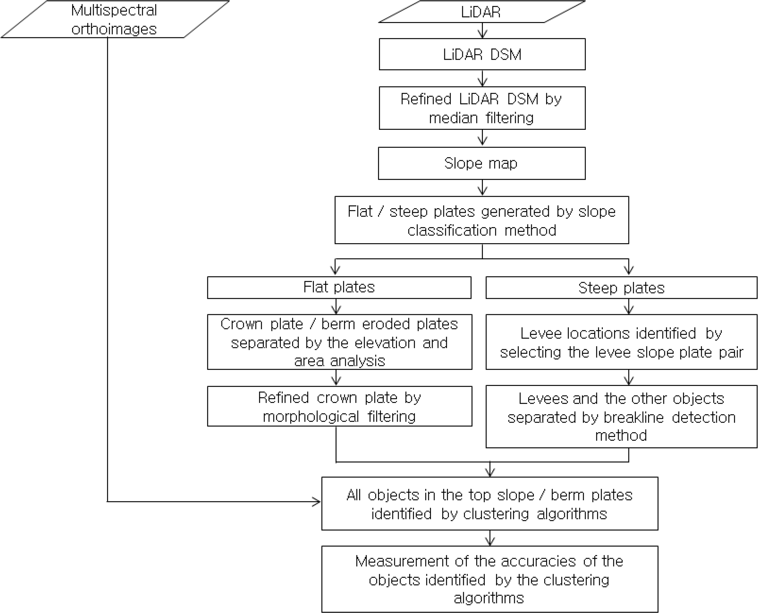
Multiple components located on the levees have different spectral and geometric patterns that can be identified using multiple analysis methods. Figure 3 shows the procedure for mapping these surfaces. The procedure includes multiple steps such as slope classification method, elevation and area analysis, median filtering, morphological filtering, clustering algorithms, and the breakline detection method for mapping levees.
In the diagram shown in Figure 3, the LiDAR Digital Surface Model (DSM) is generated using the linear interpolation method. Then, the slope map is generated by calculating the maximum rate of change between each pixel and its neighbors. The flat and steep polygons are generated separately from the slope map using the slope classification method. The levee locations are identified by manually selecting the slope polygon pairs from the steep polygons. The breakline detection method is applied to distinguish the levee slope polygons and other objects. The elevation and area analysis is carried out to separate the crown polygon, berm, and eroded polygons. Morphological filtering is applied to refine the original crown polygon. Using this procedure, the crown, slope, berm, and eroded polygons with different geometric patterns are identified. Then, the major objects on the levees, such as the asphalt, gravel, and soil roads on the crown and berm polygons, and the concrete, soil, and vegetation on the slope polygons, are identified using the clustering algorithms. Finally, the multiple components, such as the major objects and the eroded areas on the levee surfaces with different spectral and geometric patterns, are identified, and the accuracy of the identified objects is measured.
3.1. Generating Slope Maps
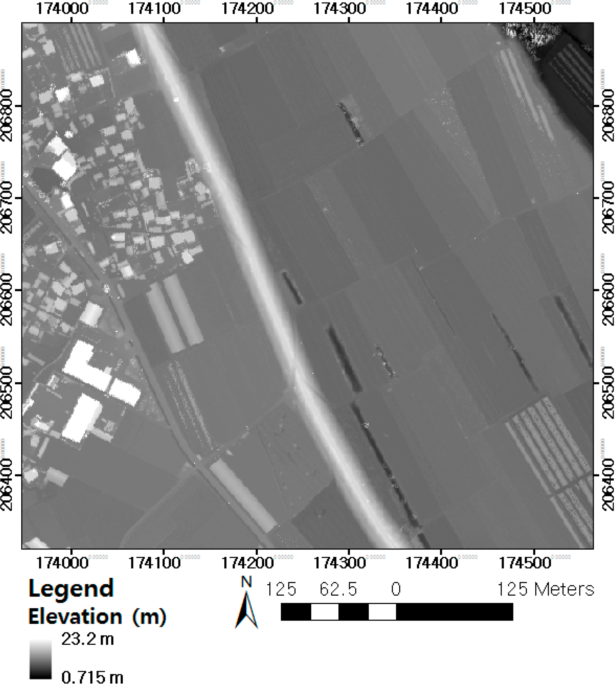
The LiDAR data consists of the irregularly distributed points. To represent the topographic surfaces using the grid format that consists of the constant cells, the DSM is generated from the given LiDAR point cloud (the point density of the given LiDAR data: 1.5 points/m2). The interpolation method is employed to estimate the elevation of each cell in the generated LiDAR DSM. In general, slopes are significantly changed at the levee crown and toe surfaces. Hence, to detect the levee crown and slope surfaces, the linear interpolation method is used to generate the LiDAR DSM, since it has characteristics that can describe the features, sharp edges, and steep surfaces [12]. The point density of the LiDAR data plays an important role in determining the grid resolution of the created LiDAR DSM. There is no reference by which to calculate the grid resolution of the DSM as a function of the point density of LiDAR data. In this research, a 1 m resolution is set as the grid resolution of the DSM to make sure that each cell of the DSM includes at least one LiDAR point. Figure 4 shows one section of the LiDAR DSM generated from the LiDAR points using the linear interpolation method. In Figure 4, the objects with brightly colored pixels are relatively higher in elevation than the neighboring pixels.
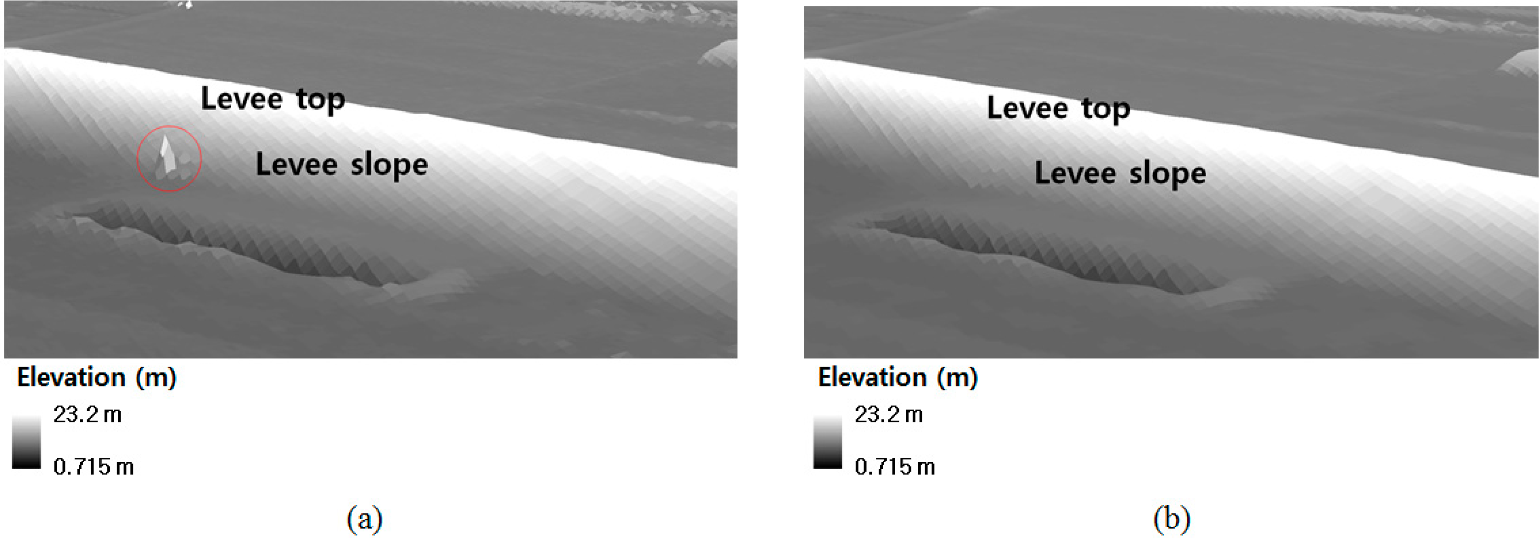
In general, the LiDAR DSM often includes outliers, which are the pixels that are significantly different in elevation compared with all the nearby pixels. These outliers are caused by random errors or objects such as utility poles, and these outliers, located near the levees, can cause difficulty when trying to detect levee mounds, which generally have gradual slopes. To remove these nearby outliers and to preserve the mounds that make up the levee’s crown and slope surfaces, filtering is employed. Research on minimizing these outliers by filtering to extract the coastal features has been carried out by Liu et al. [13] and Choung et al. [14]. In their research, a median filter was employed, which is a non-linear filter based on neighborhood ranking [15,16]. The major advantages of median filtering over other linear filters are eliminating points with much larger values than the immediate neighboring points, and avoiding data modification [13,15]. Figure 5 shows a refinement of the LiDAR DSM using the median filter: (a) one section of the original LiDAR DSM that includes the outlier (the feature in the red circles); and (b) one section of the refined LiDAR DSM that does not have the outlier after the median filtering.
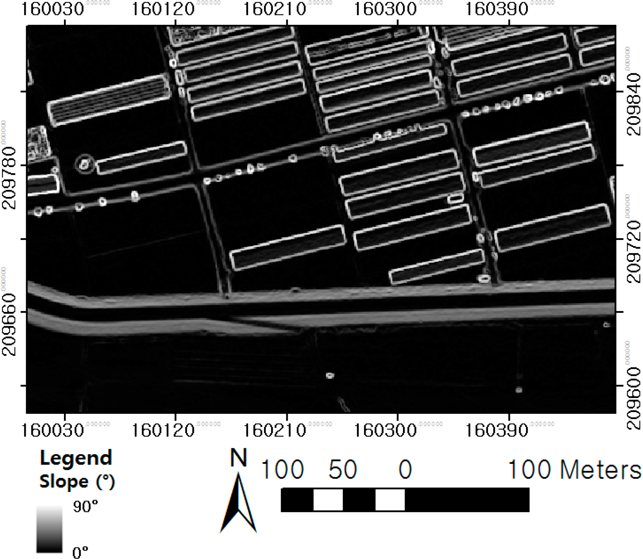
In Figure 5, the outliers located near the levees in the raw LiDAR DSM (see Figure 5a) are removed, and the mounds that consist of the levee’s top and slope surfaces are preserved in the refined LiDAR DSM (see Figure 5b). The next step is to generate the slope map from the refined LiDAR DSM by calculating the maximum rates of elevation difference between each pixel of the refined LiDAR DSM and its neighboring pixels. In the generated slope map, an intensity value for each pixel represents the slope degree of the area. In general, the pixels with low slope values represent the objects that have relatively flat terrains, and the pixels with high slope values represent the objects that have relatively steep terrains. Figure 6 shows one section of the generated slope map.
3.2. Generating the Levee Component Polygons
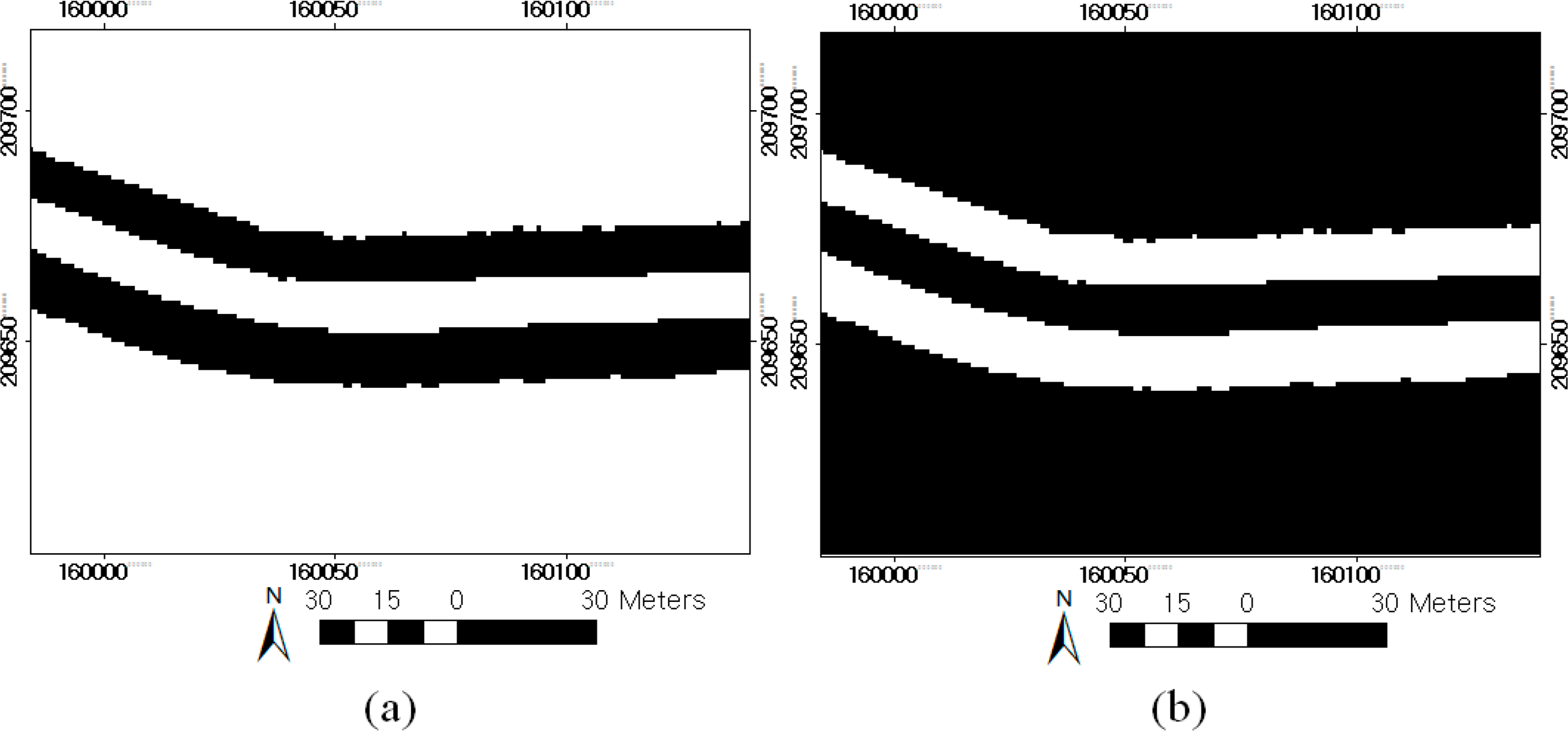
Typical levees consist of steep surfaces with elevations that gradually increase from the toe to the crown on their surfaces, and flat surfaces with stable surface elevations. Steep and flat surfaces are separately generated from the slope map using the slope classification method. Historically, the levees constructed in South Korea are designed to have slope degrees from 18.43° (1V (Vertical):3H (Horizontal)) to 33.69° (1V:1.5H) on their slope surfaces [2,5]. Considering the geometric changes, such as erosion occurring on the levee slope surfaces, ±10° is added to the slope degree range for selecting the pixels representing the levee slope surfaces. Hence, the slope degree range for generating steep areas, including the levee slope surfaces, is set as [8.43°, 43.69°]. The slope degree range for the extraction of flat areas, including the levee crown surfaces, is set to avoid the first range and uses the lower degree values. Hence, it is set as [0°, 8.43°]. Using the above two ranges, the two types of areas are separately generated from the slope map. In this research, the binary image generated using the first slope degree range is called the steep area image, and the binary image generated using the second slope degree range is called the flat area image. In general, the steep area image shows the objects that have steep terrains, such as the levee slope surfaces, and the building walls, while the flat area image shows the objects that have flat terrains, such as the natural ground, the levee crown surfaces, highways, and roofs. The flat and steep area images separately generated from the slope map, using the slope classification method, are shown in Figure 7.
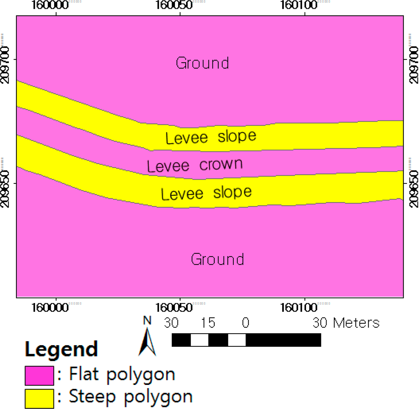
Figure 8 shows the flat polygons (pink polygons) selected from the flat area image, and the steep polygons (yellow polygons) selected from the steep area image.
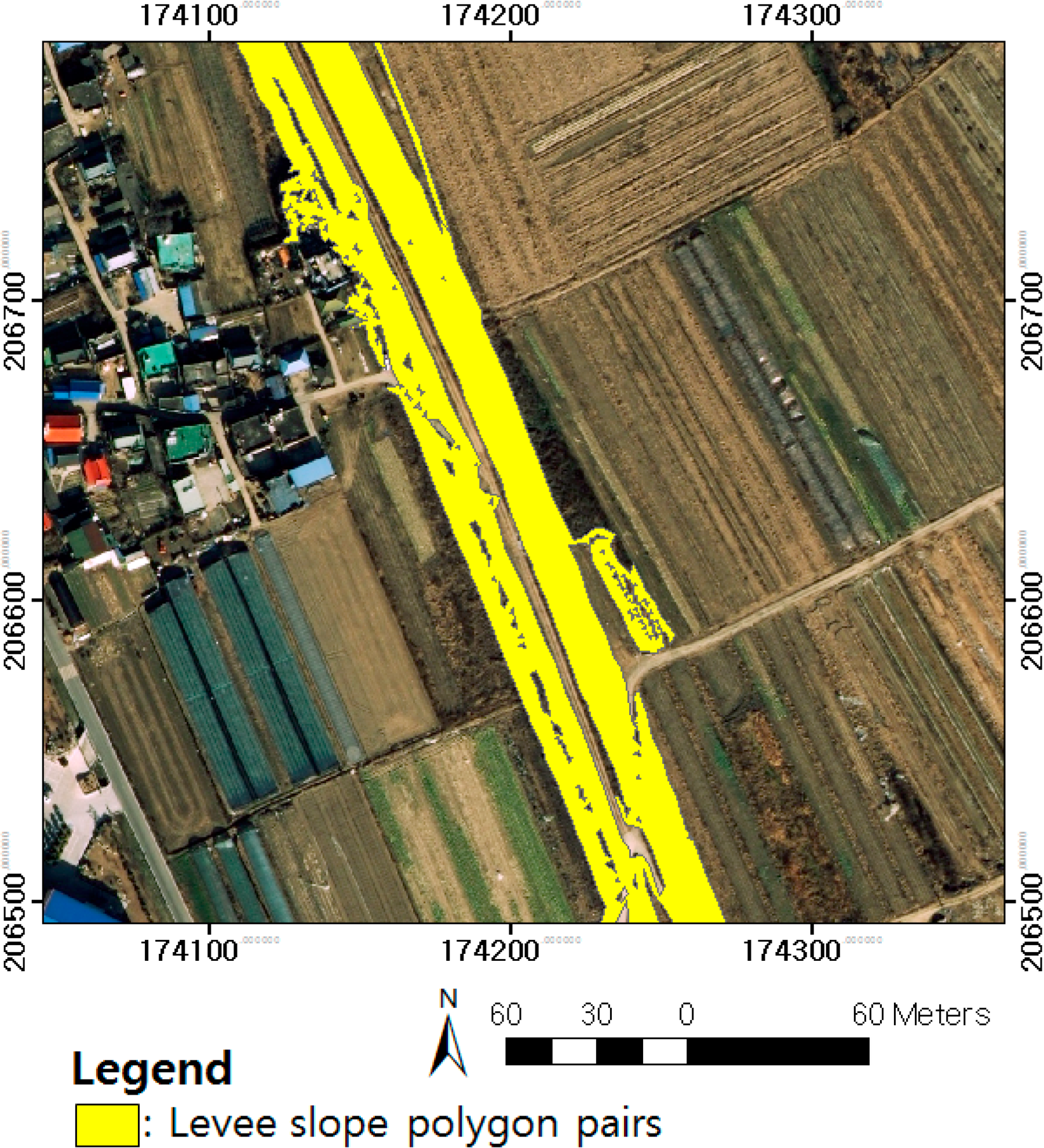
In Figures 7 and 8, the levee crown polygons and the ground are identified in the flat area images, and the levee slope polygons are identified in the steep area images. The levees have different geometric characteristics from the objects such as highways or bridges because the levee mounds consist of the slope surfaces on both sides and are located along a river’s course. Hence, the steep surfaces that represent the levee slope polygon pair are manually selected from the steep area image to identify the levee locations in the study areas. Figure 9 shows an example of the selected levee slope polygon pairs (yellow polygons).
In Figure 9, some areas of the levee slope polygons (yellow polygons) are not separated from the neighboring objects (houses, trees, buildings, etc.) located near the levees. Additionally, the levee toes generally have sharp edges because their surfaces are usually cut by the water flow [17], and the levees are designed to have certain degrees on their slope surfaces. Hence, for detecting the levee boundaries generally located at the sharp edges of the toe surfaces and for distinguishing between the levee slope polygons and the neighboring objects, the breakline detection method is employed. In this research, the breakline detection method developed by Choung et al. [14] is employed for mapping the levee boundaries. The method is a semi-automatic method for constructing a 3D breakline from the LiDAR data by connecting manually selected line segments. This method is efficient for detecting the line segments located at the sharp edges (step or ramp edges) of coastal features such as blufflines [14]. This method includes the following multiple steps. First, median filtering is applied to the LiDAR points to remove the outliers, which are significantly different in elevation compared with the neighboring points. Second, the Delaunay triangulation networks are constructed using the LiDAR points located in the levee slope polygons. The next step is to find an edge that serves as a levee toe line candidate by examining the orientation of the two surface triangles that intersect at this edge. Using the above procedure, Method 1 and Method 2 are employed to extract the levee toe edges from the vectors. Below is the equation used in Method 1 and Method 2 [14].
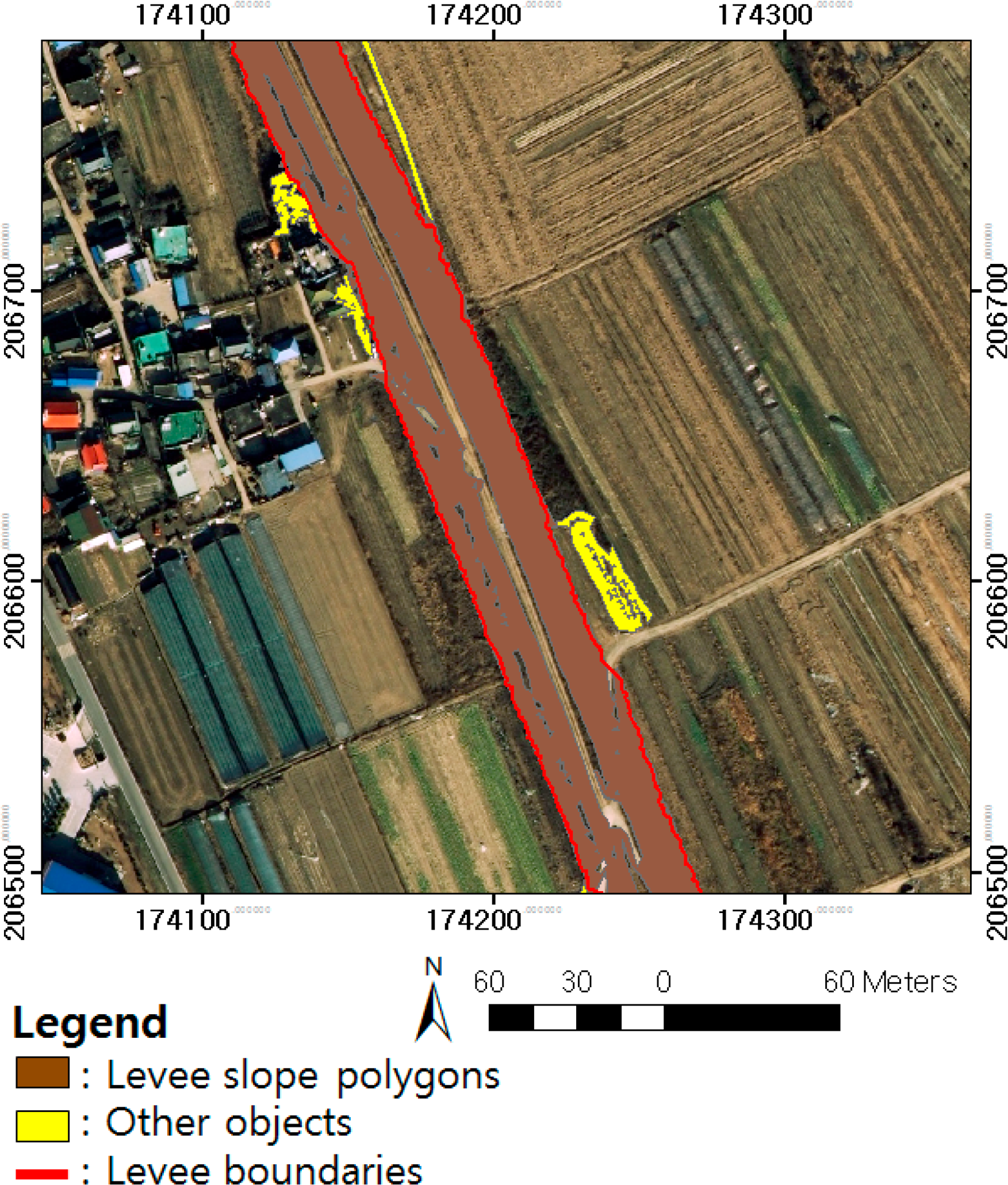
In Method 1, e is the edge of the Delaunay triangulation network, A(e) is the value of a dihedral angle defined by the two normal vectors of the two adjacent triangles, and ‖ni‖ and ‖nj‖ correspond to the norms of these two normal vectors. In Method 2, ni and nj are defined as the average normal vectors of the vertices xi and xj opposite to the edge e. These average normal vectors are computed using all the normal vectors of the triangles sharing vertices xi and xj, respectively. Using both methods, the levee toe line candidates are extracted separately, and we select a set of candidate edges, suitable for the levee toe line segment, from a combination of edge groups A and B extracted by Method 1 and Method 2, respectively. The next step is to remove the unsuitable edges with high elevation difference between the two end points, or having one end linked to the multiple edges by examining the elevation difference between the two endpoints of the edge and the edge connectivity. The final step is to manually select the line segments located in the levee slope polygons that were selected from the steep area image. Using the selected line segments, the levee boundaries are constructed by connecting the selected line segments. The generated levee boundary can separate the levee slope polygons from the neighboring objects. Figure 10 shows the levee slope polygons (brown polygons) separated from the other objects (yellow polygons) by the levee boundaries (red lines) generated by the breakline detection method.
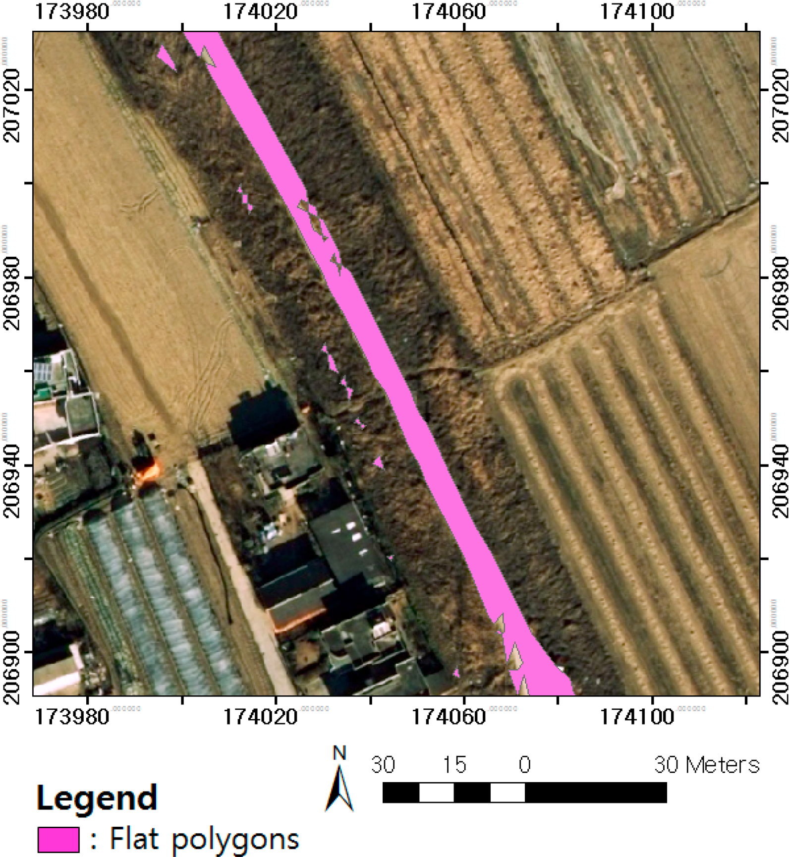
The next step is to distinguish the levee crown polygons from the multiple flat polygons extracted from the flat area images. After the levee boundaries are generated using the breakline detection method, multiple flat polygons, located between the levee boundaries, are selected. Figure 11 shows the multiple flat polygons (pink polygons) on the levee surfaces.
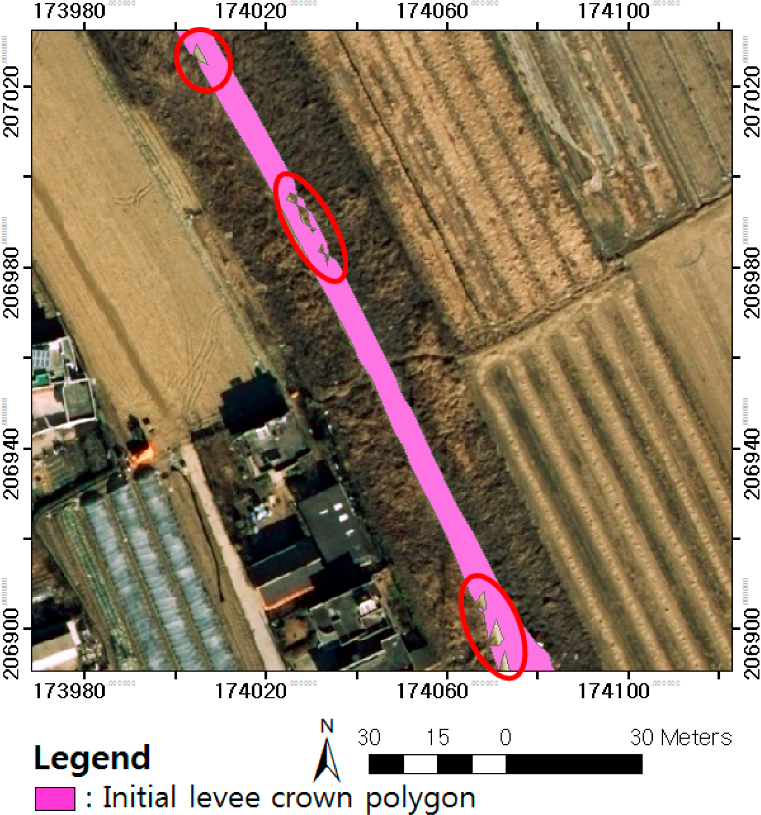
Among the multiple flat polygons shown in Figure 11, the polygon that has the highest average elevation is selected as the initial levee crown polygon. The polygons with a lower average elevation than the selected polygon are defined as the other flat polygons. Figure 12 shows the selected levee top polygon (pink polygon) having small holes, gaps, or narrow breaks on its surfaces (the red circles).
Due to the failures that generally occur on the top surfaces, the selected crown polygon often has small holes, gaps, or narrow breaks on its surface. To remove these narrow breaks, small holes, or gaps on the crown polygon, morphological filtering is applied to the initial crown polygon in the binary image. Morphological filtering is a technique for the analysis and processing of the geometric structure of the image object by creating a newly shaped object by running a specific-shaped Structure Element (SE) over the Input Object (IO) [18]. Morphological filtering has a geometric filtering property, which can preserve the geometric features of the input objects and can filter the noises in the input objects out by controlling the filter design [18]. Due to these characteristics, morphological filtering is employed to refine the initial crown polygon, which generally has linear structures.
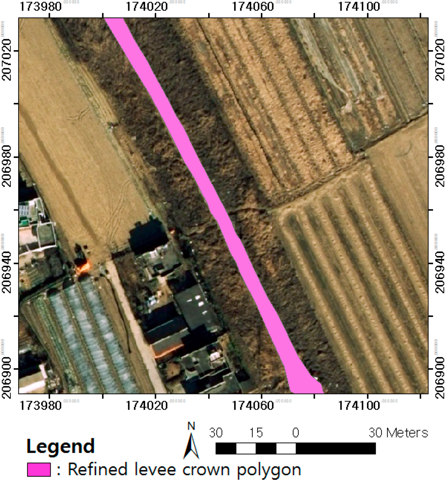
In this research, the morphological closing operator is used to fill the small holes and gaps on the selected levee crown polygon shown in Figure 12. Since the levee top polygons have a linear structure with stable widths, the shape of the SE is set as squares. To preserve the original width of the IO and fill the small holes or gaps in the IO, the width of the SE should be similar to the width of the levee crown polygon. According to the construction law from MOLIT in South Korea, the minimum width of the crown of the levees in South Korea is set as the 4 m [2,5]. Hence, the width of the SE is also set as 4 m. Figure 13 shows the refined levee top polygon (pink polygon) by using the morphological closing operator.
Compared with the initial crown polygon shown in Figure 12, the width of the refined crown polygon shown in Figure 13 is preserved. In addition, the holes or gaps in the initial crown polygon in Figure 12 are removed in the refined crown polygon shown in Figure 13. After the levee crown polygons are refined by morphological filtering, the levee berm polygons and eroded polygons are separated in the other flat polygon group. Historically, the levee berm is designed to be located 3m lower than the levee crown on the levee surfaces [5]. Considering the definition of the levee berm, we separate the levee berm polygons from the other flat polygon group by using the elevation and area analysis described in the following paragraphs.
Assumption 1: The polygon, with an elevation in the range determined by the elevation analysis, is defined as the levee berm candidate polygons and the range is determined using the following equation.
where the LBC denotes the average elevation of the levee berm candidate polygons, the LT denotes the average elevation of the levee crown polygon and the T denotes the threshold of the elevation difference between the crown polygon and the berm polygon. Due to the possible topographic changes occurring on the levee surfaces, ±1 m is added into the range to select the levee berm candidate polygons. Following the law of construction of the levee berm, the T is set as 3 m and the flat polygon, with an elevation in the above range, is identified as the levee berm candidate polygon.Assumption 2: There is no reference to the size and length of the levee berm. Since the levee berms are generally used as roads [5], we assume that they have the appropriate road geometry. Hence, we select the levee berm polygons from the candidate polygons by using the following equation.
where AB denotes the areas of the candidate polygons and TA denotes the threshold of the area. Based on an empirical analysis, the polygon with an area larger than 100 m2 is selected as the levee berm polygon, and the polygon smaller than 100 m2 is defined as the eroded polygon. Hence, the TA is set as 100.
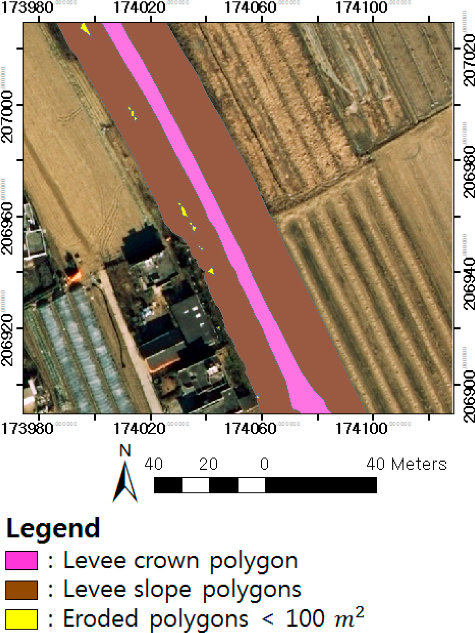
Using the elevation and area analysis described in the above paragraphs, the polygon that satisfies the above two assumptions is selected as the levee berm polygon; otherwise, it is defined as the eroded polygon. Figure 14 shows the levee crown polygon (pink), the levee slope polygons (brown) and the eroded polygons (yellow) on the levee surfaces. Figure 15, on the other hand, shows the levee crown polygons (pink), the levee slope polygons (brown) and the levee berm polygon (purple) on the levee surfaces.
Through all the procedures, the levee crown, slope, berm and eroded polygons that have different geometric patterns are identified (see Figures 14 and 15).
3.3. Identification of the Major Objects on the Levee Components
Since these objects have different spectral characteristics that can be identified in multispectral image sources, multispectral bands, such as red, green, blue and Near Infra-Red (NIR), are used for identification. In addition, the LiDAR systems also provide the intensity value for each return, and the LiDAR intensity value is determined by an object’s reflectance. This can be used to identify the land-cover classes [19]. Hence, for identification of the multiple components located on the levee surfaces, the spectral information obtained from the multispectral orthoimages and the LiDAR intensity values obtained from the LiDAR system are used as the main parameters. Clustering is a machine learning technique widely used to extract the thematic information from the multispectral images in remote sensing application and research [20–22]. It is an unsupervised learning technique for organizing the objects into multiple groups, with members that are similar in some way without the training samples [23,24]. In this research, the two traditional clustering algorithms (the K-means and the ISODATA algorithms) are used to identify the major objects located on the crown/slope/berm surfaces. Unsupervised clustering does not require the training samples to classify the clusters with similar members that have the different spectral characteristics. As each major object on the various levee surfaces has definite spectral characteristics, it is assumed that a certain sample of one object cluster cannot be included in another object cluster. For these reasons, this research employs the K-means and the ISODATA algorithms separating the clusters with cluster boundaries to identify the multiple major objects on the crown/slope/berm surfaces. In this research, the K-means clustering and the ISODATA clustering are separately employed to extract the major objects from the levee surfaces. Since the K-means clustering requires the input of the number of generated clusters, the number of necessary clusters is generated based on a priori knowledge of the multiple components covering the levee surfaces, and a priori knowledge is provided by the WAMIS website [6]. The ISODATA clustering is similar to the K-means clustering with one advantage: the ISODATA clustering allows for the different numbers of clusters, while the K-means assumes that the number of clusters is known a priori [25]. Since the ISODATA clustering is a self-organizing algorithm, it requires little human input compared to supervised classification [26].
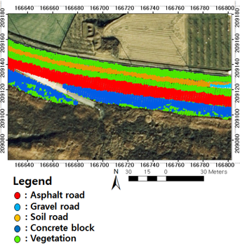
The appropriate values of each parameter are determined through multiple experiments. After the procedure is completed, several clusters are generated, and the clusters that represent the same objects are manually merged per the user’s determination. Figure 16 shows the multiple levee components (asphalt road (red), soil road or patch (orange), gravel road (cyan), concrete block (blue) and vegetation (green)) on the levee crown/slope/berm surfaces identified by the ISODATA clustering (a and b) and the K-means clustering (c and d) and the eroded areas (yellow).
4. Results and Discussion
4.1. Accuracies of the Identified Objects on Levees
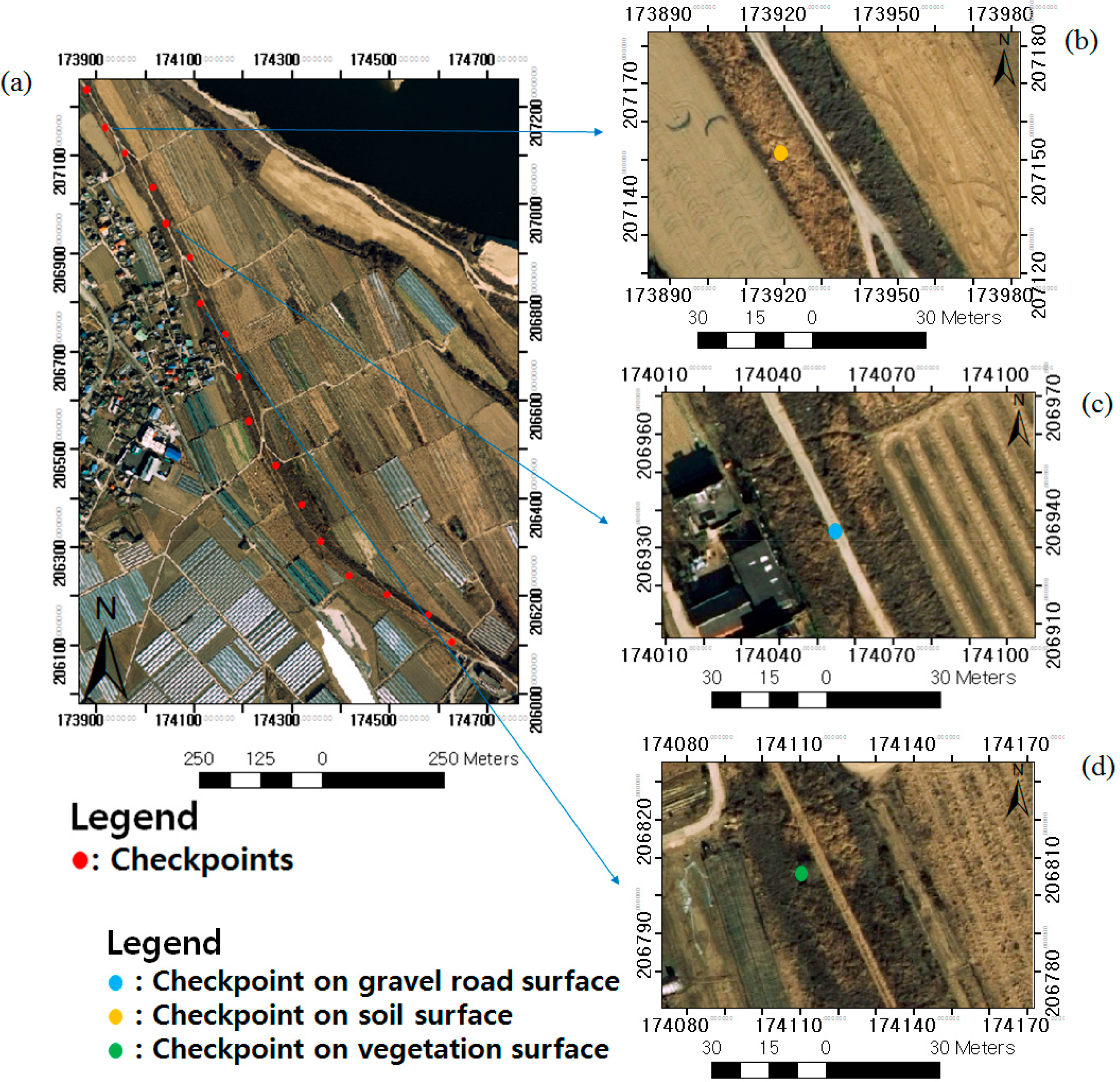
The crown and berm surfaces generally consist of the asphalt road, the gravel road, the soil road, etc., and the slope surfaces generally consist of the concrete block, vegetation, soil, etc. In this research, the accuracy of the identified objects on the levee surfaces is measured using 148 checkpoints manually determined from the aerial orthoimages by an experienced operator. The average distance between the checkpoints is 100 m. Figure 17 shows examples of the checkpoints located on the various levee surfaces.
Table 1 shows the accuracy of the identified objects generated by both clustering algorithms.
4.2. Discussion of the Accuracies and the Misclassification Errors
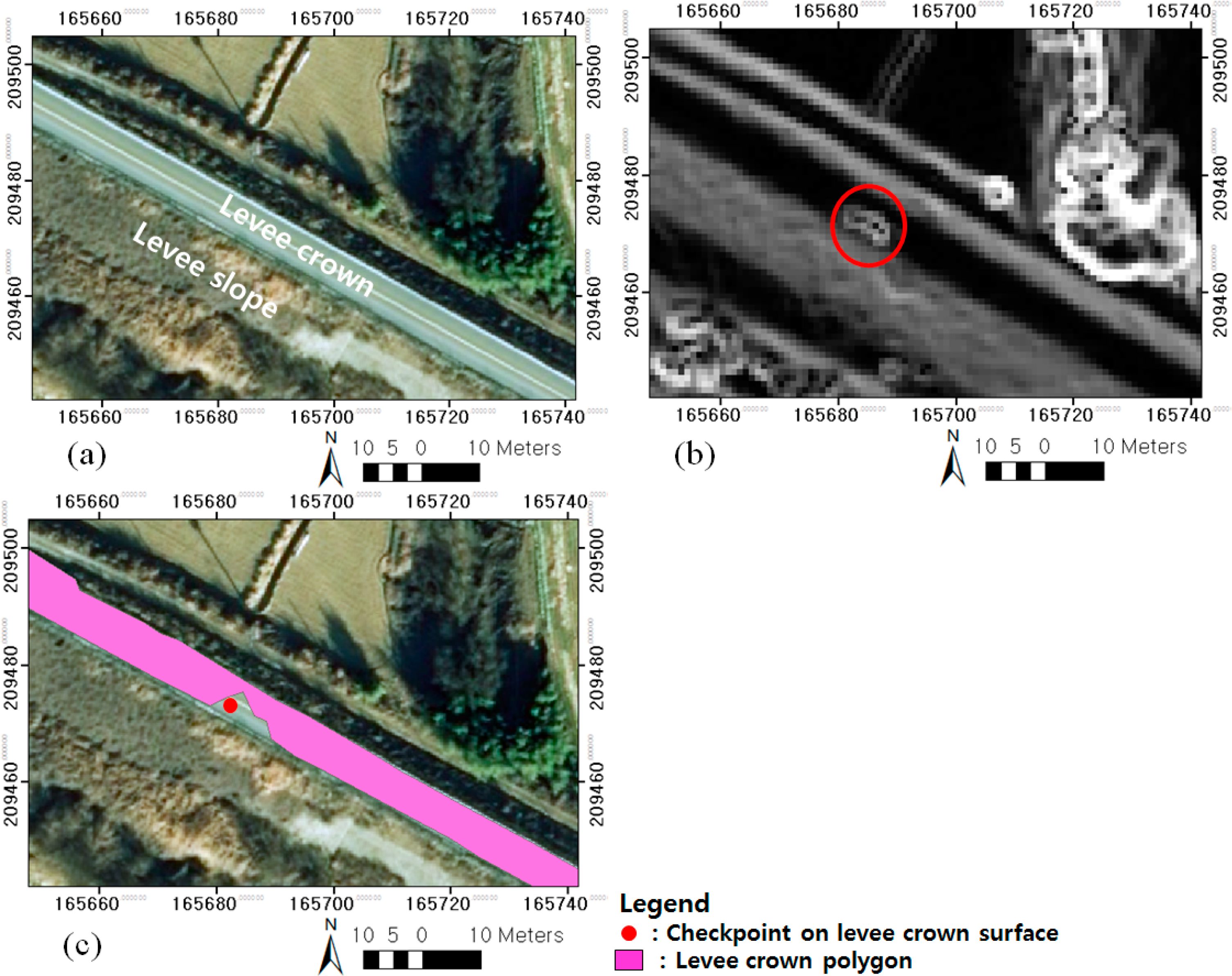
In Table 1, some misclassification errors are detected on the identified objects caused by the moving objects such as the vehicles on the levee crowns. Figure 18 shows an example of the misclassification errors caused by the moving objects.
In Figure 18a,b, moving objects are generally identified in the either data due to the different times that the two different data sets are taken. In general, the moving objects have a height higher than the levee crowns, and it causes the pixels representing the moving objects to have the slope a degree higher than the pixels representing the levee crown on the slope map (see the red circle in Figure 18b). Figure 18c shows that the shape of the generated levee crown polygon is distorted due to the moving objects on the levee crown and the area of the moving object is not classified as the area of the levee crown surface, and it causes the misclassification errors for identifying the objects on the levee crown and slope surfaces.
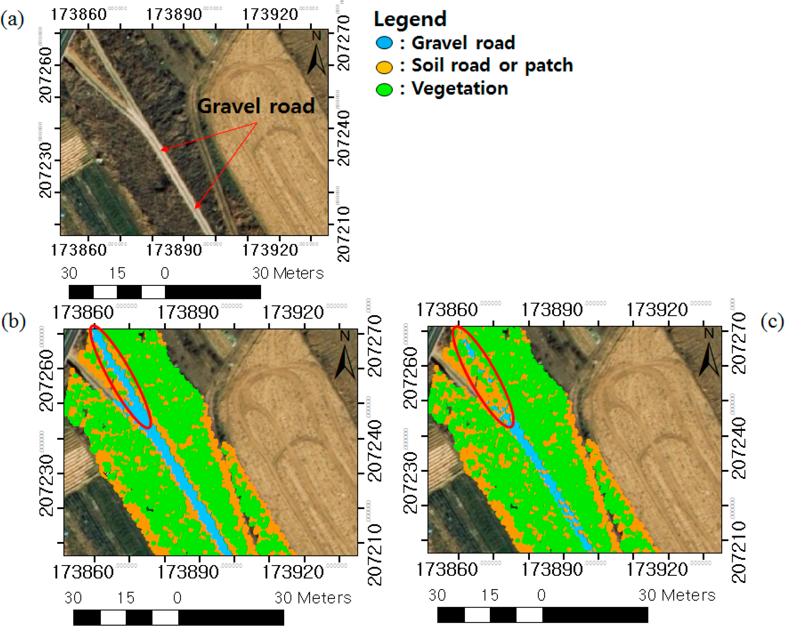
Table 1 shows that both clustering algorithms have similar accuracies for identifying artificially constructed objects such as asphalt roads and concrete blocks. In general, artificially constructed objects are visually well-distinguished and are rarely misclassified due to their paved surfaces. These characteristics also cause the artificially constructed objects to be well-identified by both clustering algorithms. The objects with the unpaved surfaces, however, such as the gravel roads, are easily misclassified as different objects such as soil roads [27]. Therefore, soil surfaces appear not only on the slope surfaces but also on the crown surfaces. These characteristics also make it difficult to determine the number of necessary clusters made by the K-means clustering. Examples of the three clusters (gravel road, soil (road or patch), and vegetation) identified by both algorithms are shown in Figure 19.
In Figure 19, some segments of the gravel roads are not classified by K-means clustering due to the misclassification of their surfaces (see the red circle in Figure 19c), while these segments are well identified as the gravel road cluster by ISODATA clustering (see the red circle in Figure 19b). In conclusion, both clustering algorithms can be used to identify artificially constructed objects with paved surfaces, while ISODATA clustering is more efficient than the K-means clustering for identifying the objects with unpaved surfaces on the levee surfaces.
4.3. Comparison of the Results with the Previous Research
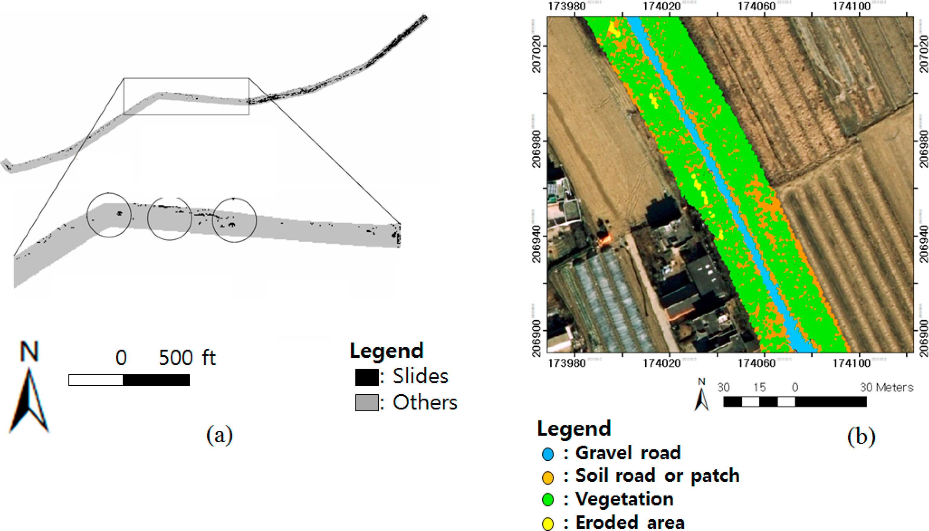
In the historical research, the spectral parameters obtained from the image sources has been used for detecting the features on levees, and it leads to the fundamental limits for mapping the multiple levee components that have the different spectral and geometric characteristics. The methodology proposed in this research is useful for identifying multiple components on levees by using the geometric and spectral information obtained from the LiDAR data and the multispectral orthoimages. Comparison of the results of multiple components on levees identified using the LiDAR data and the multispectral orthoimages by this research with the results of the slides on levees detected using the multispectral images by Hossain et al. (2006) [8] and are shown in Figure 20.
Figure 20 shows that the use of the single data is useful for detecting the specific features such as the slides on levees but limited to identify the multiple levee components having the different spectral and geometric patterns, while the use of the multiple datasets is efficient for identifying not only the single features but also the multiple levee components such as the major objects and the eroded areas on levees.
The statistical results show that the procedure introduced in this research is efficient for identifying the major objects on the levee surfaces. The accuracy of the detected geometric features (the levee crowns, the levee slopes, the levee berms and the eroded areas) on the levee surfaces can be measured by using the ground data such as the reference lines that can be obtained through the ground surveying method. However, the ground data for measuring the accuracy of the detected geometric features is currently not available, which means that it is limited to compare the geometric features with the ground data in this study.
4.4. Discussion of Assessing Stability of the Levees in the Study Area
This section discusses the evaluation of the physical condition of levees using the results obtained by this research. The physical condition of levees is evaluated by using the following equations.
In Table 2, Levees 1, 2 and 3 have the good physical condition due to the relatively small eroded areas on their surfaces, while Levees 4, 5, 6, 7 and 8 have a bad physical condition due to the relatively large eroded areas on their surfaces. Table 2 shows that the results obtained in this research can be used to evaluate the physical condition of levees to assess levee stability without human accessibility.
5. Conclusions and Future Works
Mapping levees is important for identifying multiple levee components, analyzing levee surfaces, and assessing levee stability. The use of a single data set is limited to map levees due to the different geometric and spectral patterns of the various components on levee surfaces. This research proposes a new methodology for mapping levees using geometric and spectral parameters obtained from the LiDAR data and the multispectral orthoimages by multiple geometric and spectral analysis techniques, such as the breakline detection method, morphological filtering, the 2-D interpolation method, median filtering, clustering algorithms, the slope classification method, and elevation and area analysis. This research contributes to mapping levees that consist of the various components using both geometric and spectral parameters obtained from the LiDAR data and the multispectral orthoimages taken in the Nakdong River Basins, South Korea. The ISODATA clustering has 86% overall accuracy for identifying the objects on levees, while the K-means clustering has 81% overall accuracy. This research shows that the ISODATA clustering has higher accuracy than K-means clustering for identifying the objects on levees, due to the unpaved surfaces that are easily misclassified as other surfaces. In addition, the physical condition of the levees in the study area is evaluated by using the levee components identified in this research. As seen in Figure 1, levees consist of area-based features such as the levee crown, the levee slopes and the line-based features such as the levee lines. Mapping levee lines is also important for evaluating erosion on levees and assessing stability of levees, and the results obtained in this research can be used in research on mapping levee lines. Hence, the work to be performed in the future is to map levee lines using the results obtained in this research.
Acknowledgments
The author would like to thank Rongxing Li for his academic help. This research was funded by the research project of flood defense technology for next generation.
Conflicts of Interest
The author declares no conflict of interest.
References
- FEMA Levee Resources and Library. Available online: http://www.fema.gov/living-levees-its-shared-responsibility/fema-levee-resources-library (accessed on 5 May 2014).
- Lee, J.S. River Engineering and Design; Saeron Books: Seoul, Korea, 2010. [Google Scholar]
- Design and Construction of Levees. Available online: http://www.publications.usace.army.mil/Portals/76/Publications/EngineerManuals/EM_1110-2-1913.pdf (accessed on 5 May 2014).
- Levee Inspection. Available online: http://www.usace.army.mil/Missions/CivilWorks/LeveeSafetyProgram/LeveeInspections.aspx (accessed on 5 May 2013).
- Documents for Management of Nakdong River Basins in 2009. Available online: http://www.river.go.kr/WebForm/sub_04/sub_04_01_01.aspx (assessed on 5 May 2014).
- Database of the Levees in Nakdong River. Available online: http://www.wamis.go.kr/WKF/wkf_banksaa_lst.aspx (assessed on 5 May 2014).
- Bishop, M.J.; McGill, T.E.; Taylor, S.R. Processing of Laser Radar data for the extraction of an along-the-levee-crown elevation profile for levee remediation studies. Proc. SPIE 2004, 5412, 354–359. [Google Scholar]
- Hossain, A.; Easson, G.; Hasan, K. Detection of levee slides using commercially available remotely sensed data. Environ. Eng. Geosic 2006, 12, 235–246. [Google Scholar]
- Mahrooghy, M.; Aanstoos, J.; Parasad, S.; Younan, N.H. On land slide detection using terrasar-x over earthen levees. Int. Arch. Photogramm. Remote Sens. Spat. Inf. Sci 2012, 39, 497–501. [Google Scholar]
- Hossasin, A.; Easson, G. Predicting shallow surficial failures in the Mississippi River levee system using airborne hyperspectral imagery. Geomat. Nat. Hazard. Risk 2012, 3, 55–78. [Google Scholar]
- Estimated Values Damages by Flooding. Available online: http://www.wamis.go.kr/wkf/wkf_fddamaa_lst.aspx (accessed on 5 May 2014).
- A Review of Spatial Interpolation Method for Environmental Scientists. Available online: http://www.ga.gov.au/image_cache/GA12526.pdf (accessed on 5 May 2014).
- Liu, J.-K.; Li, R.; Deshpande, S.; Niu, X.; Shih, T.-Y. Estimation of blufflines using topographic LiDAR data and orthoimages. Photogramm. Eng. Remote Sens 2009, 75, 69–79. [Google Scholar]
- Choung, Y.; Li, R.; Jo, M.-H. Development of a vector-based method for coastal bluffline mapping using LiDAR data and a comparison study in the area of Lake Erie. Mar. Geod 2013, 36, 285–302. [Google Scholar]
- Schenk, T. Digital Photogrammetry, Volume I: Background, Fundamentals, Automatic Orientation Procedures; Terra Science: Laurelville, OH, USA, 1999. [Google Scholar]
- Wolf, P.R.; Dewitt, B.A. Elements of Photogrammetry with Applications in GIS, 3rd ed.; McGraw-Hill: New York, NY, USA, 2000. [Google Scholar]
- Levee Owner’s Manual for Non-Federal Flood Control Works. Available online: http://www.nws.usace.army.mil/Portals/27/docs/emergency/LeveeOwnersManual%28final%29.pdf (accessed on 5 May 2014).
- Gonzalez, R.C.; Woods, R.E. Digital Image Processing, 3rd ed.; Pearson Education Inc.: Upper Saddle River, NJ, USA, 2008; p. 976. [Google Scholar]
- Wang, C.; Glenn, N.F. Integrating LiDAR intensity and elevation data for terrain characterization in a forested area. IEEE Geosci. Remote Sens. Lett 2009, 6, 463–466. [Google Scholar]
- Asmus, V.; Buchenev, A.; Pyatkin, V. Cluster analysis of earth remote sensing data. Optoelectron. Instrum. Data Process 2010, 46, 149–155. [Google Scholar]
- Jensen, J.R. Introductory Digital Image Processing (A Remote Sensing Perspective), 3rd ed; Prentice-Hall Series in Geographic Information Science: Upper Saddle River, NJ, USA, 2004. [Google Scholar]
- Xu, H.; Li, X.; Gao, X. Clustering analysis as a basic tool for hyperspectral remote sensing image. Proc. SPIE 2011. [Google Scholar] [CrossRef]
- Halder, A.; Ghosh, A.; Ghosh, S. Supervised and unsupervised map generation from remote sensed images using ant based systems. Appl. Soft Comput 2011, 11, 5770–5781. [Google Scholar]
- Tuia, D. Semisupervised remote sensing image classification with cluster kernels. IEEE Geosci. Remote Sens. Lett 2009, 6, 224–228. [Google Scholar]
- Ahmad, A.; Sufahani, S.F. Analysis of Landsat 5 TM data of Malaysian land covers using ISODATA clustering technique. Proceeding of 2012 IEEE Asia-Pacific Conference on Applied Electromagnetics (APACE 2012), Melaka, Malaysia, 11–13 December 2012; pp. 92–97.
- Li, B.; Zhao, H.; Lv, Z. Parallel ISODATA clustering of remote sensing images based on Mapreduce. Proceeding of the 2010 International Conference on Cyber-Enabled Distributed Computing and Knowledge Discovery, Huangshan, China, 10–12 October 2010; pp. 380–383.
- Section I: Routine Maintenance and Rehabilitation. Available online: http://water.epa.gov/polwaste/nps/upload/2003_07_24_NPS_gravelroads_sec1.pdf (accessed on 5 May 2013).


| K-Means | ISODATA | ||||||
|---|---|---|---|---|---|---|---|
| Overall Accuracy | 81% | Overall Accuracy | 86% | ||||
| Producer’s Accuracy | User’s Accuracy | Producer’s Accuracy | User’s Accuracy | ||||
| Asphalt Road | 87% | Asphalt Road | 100% | Asphalt Road | 87% | Asphalt Road | 100% |
| Gravel Road | 88% | Gravel Road | 84% | Gravel Road | 88% | Gravel Road | 91% |
| Concrete on slopes | 89% | Concrete on slopes | 93% | Concrete on slopes | 86% | Concrete on slopes | 93% |
| Vegetation on slopes | 84% | Vegetation on slopes | 77% | Vegetation on slopes | 86% | Vegetation on slopes | 83% |
| Soil (road or slopes) | 60% | Soil (road or slopes) | 67% | Soil (road or slopes) | 83% | Soil (road or slopes) | 75% |
| Levee ID | Physical Condition | Levee ID | Physical Condition |
|---|---|---|---|
| 1 | Good | 5 | Bad |
| 2 | Good | 6 | Bad |
| 3 | Good | 7 | Bad |
| 4 | Bad | 8 | Bad |
© 2014 by the authors; licensee MDPI, Basel, Switzerland This article is an open access article distributed under the terms and conditions of the Creative Commons Attribution license (http://creativecommons.org/licenses/by/3.0/).
Share and Cite
Choung, Y. Mapping Levees Using LiDAR Data and Multispectral Orthoimages in the Nakdong River Basins, South Korea. Remote Sens. 2014, 6, 8696-8717. https://doi.org/10.3390/rs6098696
Choung Y. Mapping Levees Using LiDAR Data and Multispectral Orthoimages in the Nakdong River Basins, South Korea. Remote Sensing. 2014; 6(9):8696-8717. https://doi.org/10.3390/rs6098696
Chicago/Turabian StyleChoung, Yunjae. 2014. "Mapping Levees Using LiDAR Data and Multispectral Orthoimages in the Nakdong River Basins, South Korea" Remote Sensing 6, no. 9: 8696-8717. https://doi.org/10.3390/rs6098696
APA StyleChoung, Y. (2014). Mapping Levees Using LiDAR Data and Multispectral Orthoimages in the Nakdong River Basins, South Korea. Remote Sensing, 6(9), 8696-8717. https://doi.org/10.3390/rs6098696