1. Introduction
Nutrients and various chemicals are usually supplied to agricultural soils to improve the crop yield. Excessive use of fertilizers (including nitrogen, N) should be avoided to minimize environmental impacts. In fact, although N fertilization improves plant development, the fate of the non-absorbed portion arouses concerns due to leaching phenomena and to the emissions in the atmosphere [
1] of greenhouse gases such as dinitrogen monoxide (N
2O). However, even if the use of N fertilizers can be reduced without significantly influence the final yield [
2], farmers often administer N supplies in excess in order to avoid any N deficit and assure profits at the end of the season [
3]. To avoid such an excessive fertilization, one of the most important steps at European level was the Nitrate Directive (91/676/EEC) in 1991 concerning the protection of ground and surface waters against pollution caused by nitrates (NO
3−) from agricultural sources. This directive imposed the identification of waters containing more than 50 mg L
−1 of NO
3− (or that could contain this concentration if no action is taken to reverse the trend), and the adoption of action programmes on these vulnerable areas. The last European Commission report on the implementation of this directive for the period 2008–2011 states that the consumption of chemical fertilizers is decreasing.
A tool for the in-season detection of N deficient areas is needed in order to administer the fertilizers only where necessary. In this context, the concept of critical N concentration (%N
c) [
4,
5] was proposed as the minimum N concentration in shoots required to produce the maximum aerial biomass at a given time. The %N
c declines exponentially as a function of aboveground dry mass accumulation (W). Species-specific relationships between %N
c and W have been proposed as references to be compared with actual %N
c and W measurements to derive the crop-specific N needs at each growth stage. Nitrogen needs are formalized by means of the Nitrogen Nutrition Index (NNI) [
6,
7] defined as the ratio between the actual leaf N concentration (%N
a) measured in the field at a specific growth stage and the %N
c predicted by the reference function %N
c =
f(W). NNI values close to 1 indicate plants not limited by N availability, while values lower or higher than 1 indicate N deficiency or excessive fertilization, respectively [
6].
NNI is traditionally calculated through field measurements that are quite time consuming. As a result, a reduced number of plants is usually sampled and the spatial heterogeneity of N needs is poorly represented. The estimation of the NNI based on spectral data has been proven feasible using field spectrometers operated on the ground [
8] or mounted on tractors [
9]. However the possibility to detect the N status using remotely rather than proximal sensed information has still to be tested [
10]. The precise and effective remotely sensed estimation of the NNI input parameters (
i.e., %N
a and W) would provide a cost-effective detailed spatial characterization in order to produce maps of crop nutritional deficit.
Several studies demonstrated that leaf chlorophyll concentration can be estimated through hyperspectral vegetation indices based on the visible and red edge (680–760 nm) spectral domains [
11–
15]. Hyperspectral sensors are characterized by a high number of narrow and contiguous acquisition bands that allow a better description of specific portions of the electromagnetic spectrum compared to broadband sensors and, thus, better performances in biochemical parameter estimation [
16]. The correlation between leaf pigments and leaf N incorporated in chlorophyll molecular structure [
17,
18] justified the use of vegetation indices for the determination of plant N condition [
19–
24]. Moreover, hyperspectral data have been also successfully used to estimate aboveground biomass accumulation, the second input required for NNI computation, using combinations of visible and near infrared reflectance in the form of simple or normalized ratios [
25,
26]. Nevertheless, the use of remote sensing to monitor crops in precision farming is still limited although its high potentiality in providing spatially detailed information to support site-specific management. This approach would result in reduced economic costs for farmers and a reduced impact on environmental resources.
In this study we used hyperspectral remote sensing imagery to estimate the N concentration and the dry mass on the basis of relationships with field data acquired during the flight. An airborne campaign was conducted with an AISA Eagle (Specim, Oulu, Finland) hyperspectral sensor over an experimental maize field. The main goals were (i) to determine crop specific N needs from airborne data through the calculation of the NNI map and (ii) to quantify the N deficit or surplus in different areas with respect to a reference optimal N content to provide variable rate N fertilization maps. We finally proposed an empirical method based on the comparison of the N content accumulated in the aboveground dry mass in each pixel with the one found in the pixels identified as in optimal conditions by the NNI map.
2. Materials and Methods
2.1. Experimental Design
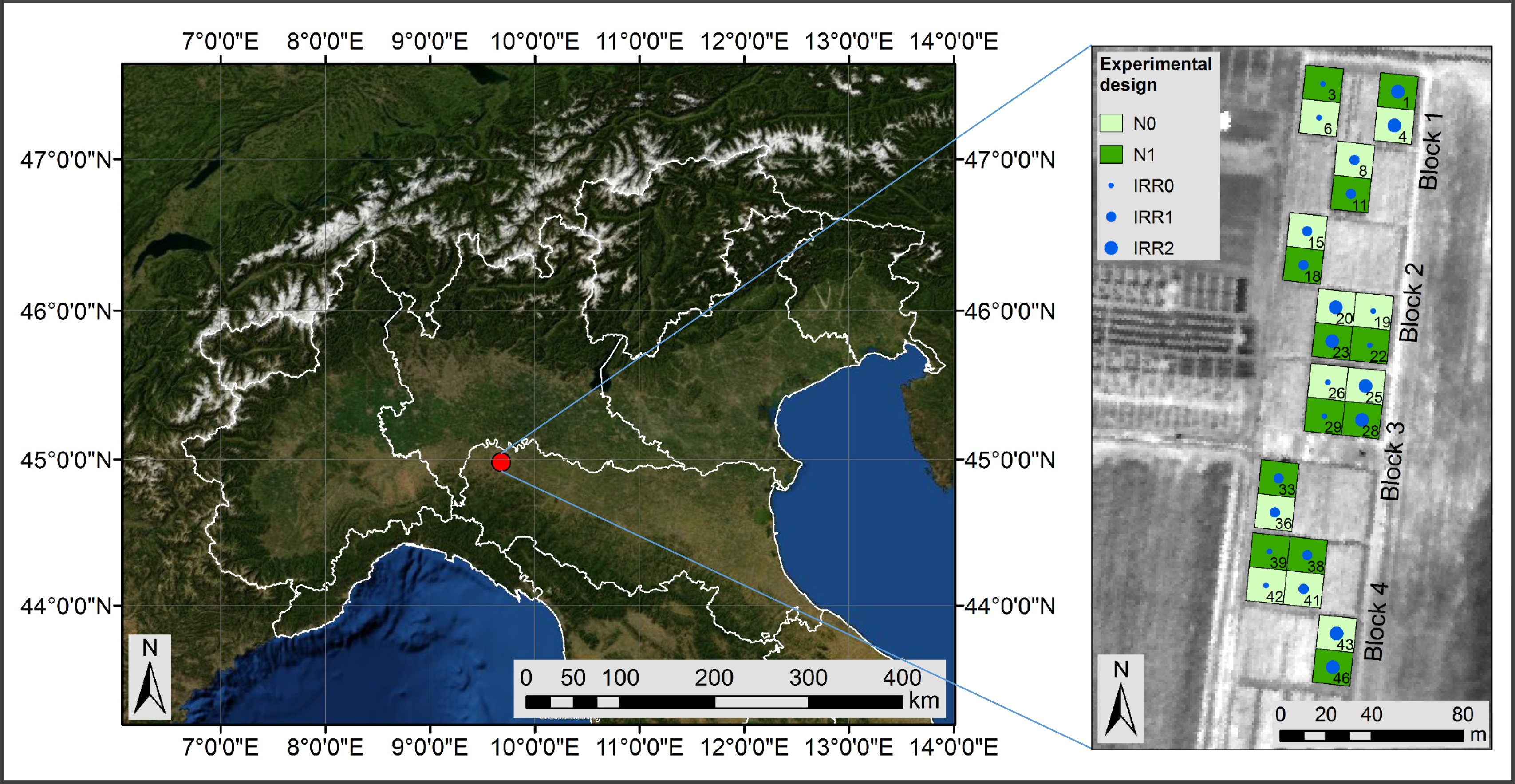
The experiment was conducted at the Vittorio Tadini experimental farm (44°58′49.0″N, 9°40′48.50″E, elevation 87 m a.s.l.) located in Gariga di Podenzano (PC) in Northern Italy.
Twenty-four maize (
Zea mays L.) plots sized 15 m × 16.5 m were organized in four replicates (blocks), as depicted in
Figure 1. In each block, two N fertilization levels (
i.e., 0 kg N ha
−1 and 100 kg N ha
−1) and three water levels (
i.e., rainfed, water deficit imposed between stem elongation and flowering and full irrigation) were randomly assigned to each plot. The water stress effects were investigated in another study [
27]. In this study, different water treatments were considered to have the effect of enhancing plant status variability, as it is expected in actual agricultural fields.
The field was sown on 3 June 2010, and N fertilizer was applied manually twenty-one days after sowing. Other information concerning the experimental management plan is reported in
Table 1.
2.2. Field Data
A field campaign was conducted contemporary to the flight on the 20 July 2010. At the time of the flight plants were in their pre-flowering stem elongation stage [
28] with an average of 10 leaves expanded.
All measurements were taken in an area of 3 m × 3 m centered in the plots. Measurements were collected through destructive (
i.e., actual N concentration (%N
a), plant dry mass and grain production) and non-destructive (
i.e., foliar measurements reported in
Table 2 and Leaf Area Index (LAI)) methods. The micro-Kjeldahl method was used to measure the %N
a from leaf samples collected immediately after the image acquisition from four plants per plot. Plant dry mass was measured immediately after the image acquisition (W
flight) in plot centers and at harvest (W
end). The %N
a and the W
flight were used for the estimation of the NNI in the field (NNI
field).
The non-destructive measurements were acquired on the last fully expanded leaf. Relative chlorophyll content (C
ab) was measured with a SPAD-502 meter (Minolta, Tokyo, Japan) [
29]. Instantaneous CO
2 assimilation (A
i) was recorded with a CIRAS-1 (PP-Systems, Amesbury, MA, USA) and photosynthetic yield (ΔF/F
m′) with a Photosynthesis Yield Analyzer Mini-PAM (Walz, Effeltrich, Germany). ΔF/F
m′ represents the efficiency of electron transport by photosystem II (PSII) under steady-state conditions of actual irradiance. Higher ΔF/F
m′ values are typical of healthier leaves: ΔF is the difference between F
m′, the maximal fluorescence yield of the sample under environment illumination and F
t, the fluorescence yield under environment illumination measured before the saturation pulse [
30]. LAI (Leaf Area Index) is the measure of the green area per soil unit area, and was estimated in each plot center using a linear ceptometer in the PAR (Photosynthetically Active Radiation) domain (SunScan Canopy Analysis System, Delta-T devices, Burwell, UK). LAI estimation with such a device requires the measurement of incident (direct and diffuse) and transmitted radiation. The incident radiation was measured from about 0.5 m above the top of the canopy in each plot. The direct to diffuse radiation ratio was then estimated by conducting a second incident radiation measurement after shadowing about 1/4 of the probe sensors (100 cm long) according to [
31]. Seven LAI measurements were then conducted and averaged along a transect crossing two consecutive crop rows, by measuring the transmitted solar radiation at ground level and exploiting the SunScan internal software for LAI estimation [
31]. For the LAI estimation from such measurements, leaf absorption in the PAR domain was assumed equal to 0.85, while the ellipsoidal leaf angle distribution parameter was set to 1.37 [
32].
2.3. Nitrogen Nutrition Index
The NNI
field [
6] was calculated with the destructive measurements conducted in plot centers contemporary to the flight. The NNI reported in
Equation (1) is the ratio between the %N
a and the %N
c as a percentage of dry mass. The %N
a is the leaf actual N concentration measured in the field and the %N
c is the minimum N concentration necessary to achieve the maximum aboveground dry mass, expressed by
Equation (2), where
a and
b are crop dependent constants and W (t ha
−1) corresponds to the plant dry mass:
According to [
33], the coefficients
a and
b were set equal to 3.40 and 0.37, respectively. NNI values close to 1 indicate plants not limited by N availability, values lower than 1 indicate N deficiency and values higher than 1 indicate that N accumulation occurs without an increase in crop biomass.
2.4. Hyperspectral Data Acquisition
A hyperspectral image was acquired at 12.37 UTC on the 20 July 2010 with the AISA Eagle sensor flown in the solar principal plane by the Italian Istituto Nazionale di Oceanografia e Geofisica Sperimentale (OGS). Acquisition parameters are given in
Table 3.
The AISA image was georeferenced with CaliGeo software (Specim, Oulu, Finland) using data from the GPS/IMU unit onboard. The image was atmospherically corrected by the empirical line approach using ground reflectance spectra measured in field at the time of the flight [
34] by means of a FieldSpec Pro portable spectroradiometer (ASD, Boulder, CO, USA). The empirical line approach is used to force image radiance (L) to match selected field reflectance spectra by means of a linear regression for each acquisition band. Two 6 m × 6 m calibration panels (white and black Odyssey material (Kayospruce, Fareham, UK)) were measured. Homogeneous targets with lambertian behaviour (two soils and one asphalt) were also measured to improve the correction accuracy [
35]. Fitting accuracy between field spectral signatures and remotely sensed data was then evaluated in each band through the Root Mean Square Error (RMSE) and resulted in less than 1% of reflectance.
2.5. Vegetation Index Computation
The plot centers were located on the AISA image and mean reflectance values were extracted from 3 × 3 pixel areas (9 m
2). Several narrowband vegetation indices were calculated. As reported in
Table 4 [
21,
36–
43], indices are divided into three categories on the basis of previous findings in literature: indices mainly related to N, to foliar pigments and to green biomass.
Two recent indices proposed for the estimation of N content, DCNI (Double-peak Canopy Nitrogen Index) and MCARI/MTVI2 (Modified Chlorophyll Absorption Ratio Index/Modified Triangular Vegetation Index 2), were tested. The following foliar pigment indices were considered: TCARI (Transformed Chlorophyll Absorption in Reflectance Index), MTCI (MERIS Terrestrial Chlorophyll Index), and TCI (Triangular Chlorophyll Index). In addition, NDVI (Normalized Difference Vegetation Index) and soil adjusted vegetation indices OSAVI (Optimized Soil Adjusted Vegetation Index), MSAVI (Modified Soil Adjusted Vegetation Index), and MTVI2 were tested as greenness indices. The combination of foliar pigment indices with soil adjusted vegetation indices was also tested as indicator of foliar pigments with the aim of normalizing for differences in canopy structure and soil contribution.
2.6. NNI and Variable Rate N Fertilization Maps
The regression analyses between field data and vegetation indices allowed the selection of the best indices for the estimation of the NNI input parameters (i.e., %Na and W).
Once the NNI map was calculated, we proposed an empirical method to quantify the N deficit or surplus in the field (Nstatus) expressed as (g N m−2). For this purpose, the actual N content accumulated in the aboveground biomass (Nw) was calculated at pixel level as %Na × W (g m−2). The optimal Nw (Nw_opt) was calculated as the mean Nw value of pixels with NNI close to 1 (i.e., optimal NNI value). Nstatus was then calculated as the difference between Nw and Nw_opt.
This allowed to map the Nstatus at the time of the flight overpass: positive values of Nstatus indicated areas characterized by N surplus, otherwise negative values of Nstatus indicated N deficit. The N deficit represents the amount of N to be prescribed in order to provide the optimal N content to improve the maize production.
2.7. Statistical Analyses
The statistical differences between biochemical and physiological parameters measured in N0 and N1 plots were tested through the Student t test. Relationships between field data and vegetation indices were evaluated by Ordinary Least Squares (OLS) regression analyses in order to determine best indices for %Na and Wflight estimation on the basis of the higher coefficient of determination (R2). Different fitting function models were tested (i.e., linear, power, logarithmic, and exponential).
3. Results
3.1. Field Data
The statistical difference between biochemical and physiological parameters measured in N0 and N1 plots was tested. As expected higher average values occurred in N1 plots, even though differences between treatments were not always significant. Results are reported in
Table 5.
The only parameter affected by N supplied to the maize plots at the time of the flight was Cab (p = 0.028). Dry mass (Wflight) differences between fertilizations were in fact not significant, meaning that differences in N supplies did not affect plant development at this stage. Instead, some differences occurred at the end of the experiment in Wharvest (p = 0.031) and in grain production (p = 0.043).
As expected, the known relationship between N and chlorophyll content [
19,
36] was confirmed in our data, since a statistically significant relationship (
p < 0.05) was found between %N
a and C
ab (
R2 = 0.56). However, contrary to C
ab, significant differences between N treatments were not detected in %N
a (
p = 0.079) and NNI
field (
p = 0.087).
3.2. Vegetation Indices Regressions
Regression analyses between field data and vegetation indices were performed to select the indices providing the best results in mapping %N
a and W, which are the input parameters for the NNI computation. The coefficients of determination and the significance of the linear regression models are reported in
Table 6; the
R2 of power, logarithmic or exponential models is reported only when it was higher than the linear one.
Combined chlorophyll indices (i.e., MCARI/MTVI2, TCARI/OSAVI, TCARI/MSAVI, TCI/OSAVI) were better related with Cab and %Na than traditional chlorophyll vegetation indices, due to the minimization of structural effects and soil contributions.
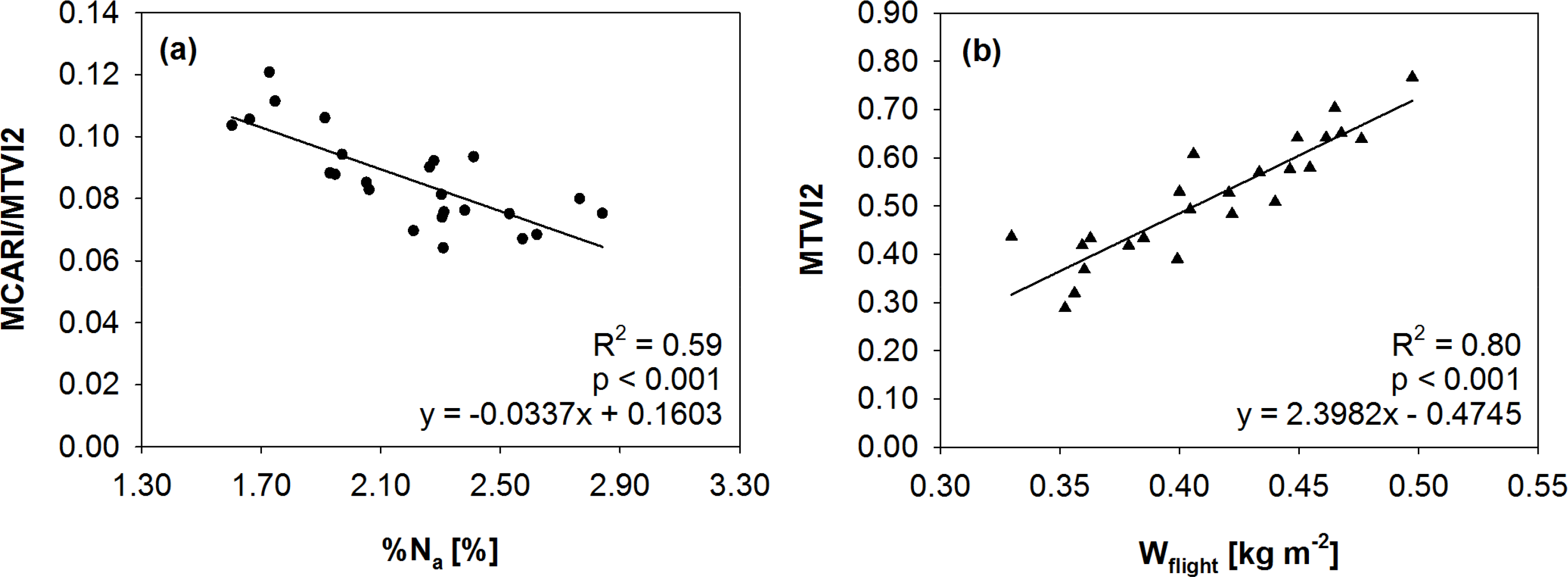
The MCARI/MTVI2 showed the best performances in estimating both C
ab (
R2 = 0.69) and %N
a (
R2 = 0.59) while it was not significantly related to LAI. This suggested that MCARI/MTVI2 was the most suitable for %N
a detection since it was not affected by canopy structure. The linear function obtained is reported in
Figure 2a. All the greenness indices were well related to W
flight (
R2 > 0.70). Soil adjusted indices (OSAVI, MSAVI, and MTVI2) performed slightly better than the traditional NDVI, since they were able to minimize the soil background effects on reflectance in case of low fractional cover. Among these the MTVI2 (
R2 = 0.80) was selected for the dry mass estimation (
Figure 2b).
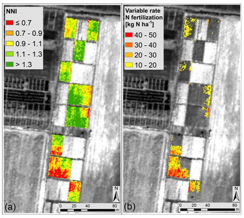
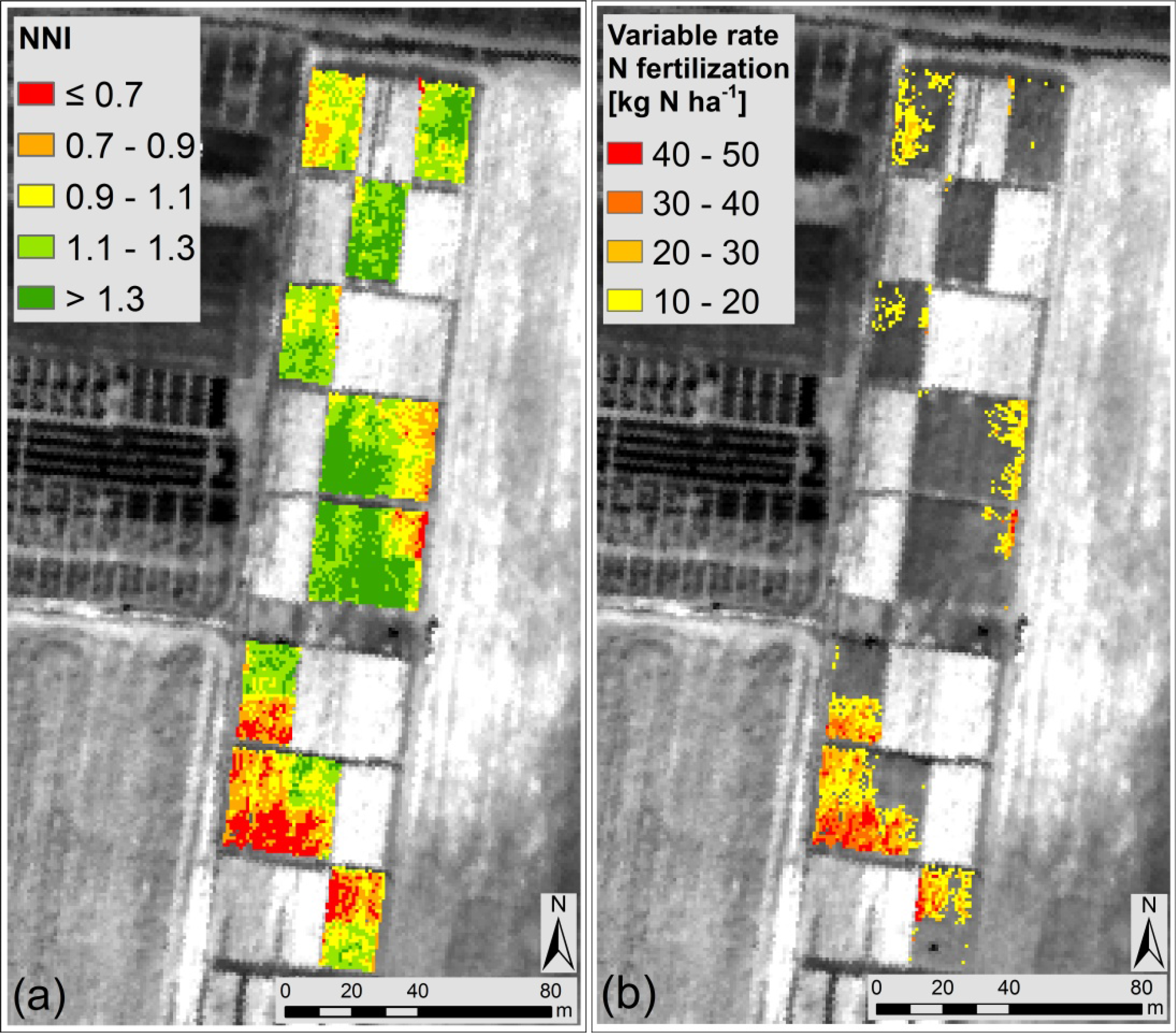
3.3. NNI and Variable Rate N Fertilization Maps
The NNI map in
Figure 3a was obtained through the combination of the input parameters (
Equations (1) and
(2)) estimated remotely with the relationships in
Figure 2. The NNI range was divided in five classes represented with colors from red (low NNI values) to dark green (high NNI values) centered around the optimal NNI value (NNI = 1). As reported in
Table 7, pixels showing N deficit (NNI ≤ 0.9) represented the 23% of the entire field, pixels with optimal N supply (0.9 < NNI ≤ 1.1) represented the 23% while pixels with N surplus (NNI > 1.1) represented the 54%.
A good agreement (R2 = 0.70, p < 0.001) was found between the mean NNI estimated for each parcel from remote sensing and the NNIfield, showing that the remote estimation of NNI is coherent with the traditional one measured in the field.
The suitability of the NNI map to detect the N status was also evaluated analysing the statistical difference between plots treated with different N amounts: the mean NNI value in N0 plots (NNI = 0.99 ± 0.23) was statistically different from the mean NNI value in N1 (NNI = 1.21 ± 0.17) (p = 0.016). It was observed that in general the field was not in a critical N deficit condition since mean values in N0 and N1 plots were both in the range of optimal N supply (i.e., NNI close to 1).
The optimal N content (N
w_opt) was computed as the mean N
w from the optimal NNI pixels (0.9 < NNI ≤ 1.1) and was found equal to 8.3 g N m
−2. This value was used together with the N
w in each pixel to estimate the N
status. Results are reported in
Table 7 for each NNI class. The N
status calculated at pixel level was converted in variable rate N fertilization (kg N ha
−1) as reported in
Figure 3b. The variable rate N fertilization quantity should allow to obtain a N
status equal to zero in each N deficient pixel, in order to reproduce the N
status typical of optimal areas. The suggested rate is shown only for pixels belonging to N deficient areas (
i.e., NNI ≤ 0.9).
4. Discussions
As observed from the field data, the availability of different N amounts did not lead to prominent visual or structural effects at the time of the image acquisition, allowing the investigation of a method for N deficiency detection in an early phase. In fact, at the time of the flight, statistically significant differences related to N supplies were observed only for Cab while the canopy structure parameters were unaffected.
Remote sensing techniques have been already used to monitor leaf chlorophyll and N concentration in agriculture in the context of precision farming practices: several studies conducted on maize crops report leaf chlorophyll concentration [
37,
39] as well as leaf N concentration maps [
36,
44] reproducing the spatial patterns related to different N supplies and soil conditions. Other studies focused on the estimation of crop density from aerial imagery [
45,
46] and from sensors onboard agricultural machineries to drive fertilization rates in real time [
47,
48]. Recently [
9] showed that spectral data collected on wheat with a tractor mounted field spectrometer were related to the NNI measured in the field. These spectral systems analyse the areas surrounding the tractor and may be a useful tool in small or medium-sized fields. However, when the field extension is considerably larger, aerial tools may become necessary. Although the attention toward precision farming techniques is increasing, studies providing methods to obtain variable rate N fertilization maps based on remote sensing data are still limited. Among remote sensing techniques it is worth mentioning the recent development of UAVs (Unmanned Aerial Vehicles) in agricultural applications allowing the collection of multispectral and hyperspectral imagery at sub-metric spatial resolution [
49–
52].
The possibility to map the NNI from airborne hyperspectral data found limited application so far; therefore, this study represents an innovative attempt to produce a variable rate N fertilization map. It should be noted that the integration of radiometric data and crop models addressed in other studies [
53] would constitute an approach able to consider also climate and soil conditions.
Our methodology allowed to merge the information about actual N concentration and dry mass identifying the areas where both parameters were low: a site-specific management was suggested over the 23% of the field, instead of an extensive fertilization. It must be noted that the proposed pragmatic approach to determine the Nstatus requires that a number of pixels with NNI close to 1 are present in the scene.
Since no recovery fertilization occurred after the flight, the deficiencies remained until the end of the growing season as shown by the differences in grain production. Even though a good agreement between NNI map and treatments was generally found, we observed some NNI values higher than 1 in few N0 plots, indicating N surplus: this could be due to nutrient residuals from previous agricultural practices. Furthermore, some low NNI values were observed in correspondence of water stressed plots (rainfed plots) even if supplied with N. This evidenced that in case water was a limiting factor plants were not able to use efficiently the supplied N and this affected the regular plant development. Remotely sensed indicators of water stress (
i.e., canopy temperature, passive fluorescence, and PRI) able to highlight conditions of critical water supply [
27,
54] might be integrated with the NNI to produce N and water variable rate maps.
In this way, knowing the amount of fertilizer administered to each parcel and the current water status, it would be possible to evaluate if the observed N deficit is due to a lack of fertilization or irrigation.
The Nstatus was quantified with reference to the average Nw shown by pixels in optimal conditions according to the NNI map (0.9 < NNI ≤ 1.1). The deficit found in the plant Nstatus was used to prescribe the amount of N that should be applied to the soil by the farmer; further investigation would be needed in order to predict the N availability for plants when fertilizers are applied to the soil, considering the losses mainly due to water leakage. Moreover, further studies should address a higher number of fertilization supplies to better evaluate the proposed method effectiveness.
5. Conclusions
This study proved that airborne hyperspectral imagery can be used to detect N deficient areas in maize crops. The parameters of interest for the production of the NNI (Nitrogen Nutrition Index) map (i.e., the leaf actual N concentration (%Na) and the dry mass (Wflight)) were successfully estimated with indices MCARI/MTVI2 (R2 = 0.69) and MTVI2 (R2 = 0.80), respectively. The obtained map constitutes an innovative attempt to calculate the NNI from airborne data over an entire field and allowed to distinguish areas characterized by different N availability (i.e., deficit, optimal and surplus). The good agreement between the NNI calculated from remote sensing and the NNI from field measurement (R2 = 0.70) supports the use of aerial data instead of traditional time consuming measurements.
The NNI map represented a crucial step for the production of a variable rate N fertilization map to be used for a rational management of the field, based on the comparison between the N accumulated in the aboveground biomass in each pixel (Nw) and the mean value of N found in optimal areas calculated through the NNI map (Nw_opt). The difference between Nw and Nw_opt (Nstatus) allowed to identify N deficit areas in correspondence of pixels where the Nstatus assumed a negative value. Only the 23% of the field was identified as N deficient and the maximum suggested fertilization rate was equal to 50 kg N ha−1. It is worth noting that the presence of vegetation in optimal conditions in the scene is necessary to compute Nw_opt and consequently Nstatus. This makes the method hardly applicable in field characterized by a widespread N deficiency where N optimal areas cannot be identified.
The method presented in this study allowed to define the minimum amount of N to apply without decreasing crop production and at the same time avoiding excessive fertilization in order to guarantee a proper management of the environmental resources in agricultural practices. Furthermore, the availability of measurements repeated over time could offer a valuable tool for a more sustainable field management during the growing season.


 ,
, 


