A Novel Clustering-Based Feature Representation for the Classification of Hyperspectral Imagery

Abstract

In this study, a new clustering-based feature extraction algorithm is proposed for the spectral-spatial classification of hyperspectral imagery. The clustering approach is able to group the high-dimensional data into a subspace by mining the salient information and suppressing the redundant information. In this way, the relationship between neighboring pixels, which was hidden in the original data, can be extracted more effectively. Specifically, in the proposed algorithm, a two-step process is adopted to make use of the clustering-based information. A clustering approach is first used to produce the initial clustering map, and, subsequently, a multiscale cluster histogram (MCH) is proposed to represent the spatial information around each pixel. In order to evaluate the robustness of the proposed MCH, four clustering techniques are employed to analyze the influence of the clustering methods. Meanwhile, the performance of the MCH is compared to three other widely used spatial features: the gray-level co-occurrence matrix (GLCM), the 3D wavelet texture, and differential morphological profiles (DMPs). The experiments conducted on four well-known hyperspectral datasets verify that the proposed MCH can significantly improve the classification accuracy, and it outperforms other commonly used spatial features.

1. Introduction

Classification, which assigns labels to pixels in the given images, is one of the most important applications of remote sensing and has been widely studied in geoscience research. A large number of studies have been conducted for the classification of remote sensing data [1–3]. The traditional pixel-based or spectral-based approaches have proved to be appropriate for the classification of low- or medium-resolution images, where spectral signals provide the predominant information for the image classification. However, with the ongoing development of Earth observation techniques, the spatial resolution of remote sensing imagery has improved a lot, and images with a higher spatial resolution provide more detail and spatial structure for the ground information [4]. In this context, spectral-based per-pixel classification methods cannot model the spatial relationship between pixels satisfactorily, and it has been widely agreed that the inherent spatial information should be exploited as a complementary feature source for classification [5].

To overcome the aforementioned problems of the spectral-only classification and to improve the processing accuracy, two main spectral-spatial analysis methods have been proposed. The first method is the object-based classification approach. In this method, the image is first segmented into a set of objects which consist of adjacent pixels with similar spectral-spatial properties, using a segmentation algorithm such as mean-shift [6], the fractal net evolution approach (FNEA) [7], watershed [8], etc. The segments/objects are viewed as the minimum image processing units for the subsequent classification. This method has been proved to be an effective approach in high-resolution remote sensing image processing [9]. On the other hand, the classification with spectral-spatial features, which incorporates the spatial features into image analysis, has attracted increasing attention since it is an effective way to complement the spectral information for the image classification [10]. The gray-level co-occurrence matrix (GLCM) is one of the commonly used features for the spectral-spatial classification [11]. With the GLCM, the textural information of each pixel is computed by the spatial correlation between the neighboring pixels in a defined window. Differential morphological profiles (DMPs) are constructed by mathematical morphological transformation and are another well-known feature for high-resolution image classification [12]. DMPs are a multiscale approach that adopts a series of morphological filters and generates a series of features with different structural elements. The use of morphological reconstruction after opening and closing can preserve the shape of the objects and suppress the undesired noisy signals. More recently, a 3D discrete wavelet transformation was proposed for urban mapping, which is suitable for describing complex urban scenes and can distinguish different information classes [13]. In addition, the shape characteristic [14], pixel shape index [15], and height information extracted from LiDAR data [16] have also been considered as complementary information for the spectral signals in image classification.

In addition to the two aforementioned methods, local frequency-based information is also an efficient strategy to exploit the spatial information and enhance the spectral classification. Gong and Howarth [17] proposed to use the gray-level occurrence frequencies to describe land-use characteristics. In [18], a frequency-based feature extraction method has been implemented on the texture spectrum for panchromatic high-resolution image classification, and led to a satisfactory accuracy. Summarizing these studies, it can be found that: (1) the image gray-level reduction, to a certain extent, can keep the salient information, remove the redundant information, and raise the computational efficiency; and (2) a local gray-level histogram is effective for representing contextual information and improving the classification. However, studies concerning local frequency feature representation are relatively rare. Moreover, it should be pointed out that the frequency-based feature representation method described in [18] is based on image gray levels, and the frequency histogram is generated band by band. In this way, when processing the hyperspectral imagery, the traditional strategy can lead to a high-dimensional histogram, which makes this technique impractical due to the computational burden and storage space.

In this context, we propose a novel multiscale cluster histogram (MCH) approach for the spectral-spatial feature representation and classification of hyperspectral data. By interpreting the relationship between the labels of the clustering map, the underlying semantic information can be excavated as the spatial feature for the spectral-spatial classification. In our work, the clustering-based feature is generated by calculating the frequencies of each cluster occurring in a set of multiscale local regions. The proposed MCH method is validated by the use of a set of public and well-known hyperspectral datasets. Moreover, its performance is compared with the commonly used spatial features of the GLCM, 3D wavelet texture, and DMPs. The rest of paper is organized as follows. Section 2 introduces the new clustering-based feature extraction approach. In Section 3, the datasets and the experimental results are presented. Finally, conclusions are drawn in Section 4.

2. Methodology

In this section, we describe the proposed MCH method (see Figure 1), which consists of three blocks: (1) clustering (generation of codes); (2) cluster histogram (spatial arrangement of codes); and (3) classification (interpretation of codes).

2.1. Clustering

The definition of clusters can be depicted as “continuous regions containing a relatively high density of points in the feature space, separated from other high-density regions”. Accordingly, clustering is a method of grouping similar objects into clusters, which makes it possible to discover the similarities and differences between the objects and to obtain the information implicated in them [19]. Let X = {x₁, x₂, … x_n} be the n pixels in a hyperspectral image, and the pixels are grouped into k clusters C = {c₁, c₂, … c_k}. The clusters should satisfy the following conditions: (1) ${\cup }_{i=1}^m{\mathit{c}}_{\mathit{i}}=\mathit{X}$; (2) c_i ∩ c_j;= ∅︀, i ≠ j, i, j = 1,2, …, k; and (3) c_i = ∅︀, i = 1,2, …, k. In spite of the fact that the clustering task can be fulfilled by various algorithms, their fundamental concepts are similar, i.e., points belonging to the same cluster are more similar to each other than points belonging to the other clusters. In this paper, the following four clustering methods are employed to generate the codes of a hyperspectral image.

(1)

K-Means: This is a centroid-based clustering method that uses the cluster centers to construct the model for the data grouping. For the sake of minimizing the sum of the distance between points to the centroid vectors, an iterative algorithm is used to modify the model until the desired result is achieved [20]. In the reassignment step, the points are assigned to their nearest cluster centroid:

$$\begin{array}{c}{\mathit{c}}_i^{(t)}=\left\{{\mathit{x}}_p:\Vert {\mathit{x}}_p-{\mathit{\mu }}_i^{(t)}\Vert <\Vert {\mathit{x}}_p-{\mathit{\mu }}_j^{(t)}\Vert \right\}\\ \forall 1\le p\le n,1\le i,j\le k,i\ne j\end{array}$$

(1)

where t represents the t-th iteration, and μ_i is the mean of the points in cluster c_i.

(2)

Iterative Self-Organizing Data Analysis Technique Algorithm (ISODATA): The basic idea of ISODATA is similar to k-means in that it minimizes the intra-cluster variability by a reassignment and update process. However, the algorithm improves on k-means by introducing a merging and splitting method during the iteration. Clusters are merged if the distance of their centers is less than a given threshold, or the number of points in a cluster is less than the predefined value. Conversely, a single cluster is divided into two clusters if the standard deviation is higher than a user-specified value, or the number of points exceeds a certain threshold. In this way, the final clustering result is obtained when all the predefined conditions are reached [21].

(3)

Fuzzy C-Means (FCM): Differing from the deterministic clustering approaches, the FCM algorithm uses a membership level to describe the relationship between points and clusters [22]. Meanwhile, the centroids of the clusters are related to the coefficients which represent the grades of membership of the clusters, and can be expressed by the weighted mean of all the points:

$${\mathit{\mu }}_i^{(t+1)}=\frac{{\sum }_{{\mathit{x}}_p\in {\mathit{c}}_i^{(t)}}{\mathit{w}}_{pi}^{(t)}{\mathit{x}}_p}{{\sum }_{{\mathit{x}}_p\in {\mathit{c}}_i^{(t)}}{\mathit{w}}_{pi}^{(t)}}$$

(2)

where w_pi is the degree of x_p belonging to cluster c_i, which is defined as:

$${\mathit{w}}_{pi}={\left(\sum _{j=1}^k{\left(\frac{\left|\right|{\mathit{x}}_p-{\mathit{\mu }}_i\left|\right|}{\left|\right|{\mathit{x}}_p-{\mathit{\mu }}_j\left|\right|}\right)}^{\frac{2}{m-1}}\right)}^{-1}$$

(3)

where m donates the level of the cluster fuzziness.

In order to obtain the cluster label of each point, the final clusters are obtained by assigning points to the cluster with the maximum membership degree.

(4)

Exception Maximization (EM) Algorithm: EM is frequently used for data clustering in machine learning, and works in two alternating steps: (1) the expectation (E) step, which refers to computing the expected value with the previous estimates of the model parameters; and (2) the maximization (M) step, which refers to altering the parameters by maximizing the expectation function [23]. The fundamental principle of the algorithm is to find a maximum likelihood estimate of the parameters through the iterative model. Each feature vector will then be assigned to one cluster on the basis of the maximum posteriori probability.

In order to reduce the computational cost of the clustering, which is related to the feature dimensionality and the cluster number, the spectral dimension should be reduced to speed up the operation [10]. Thus, a simple feature extraction method is utilized:

$${\mathit{v}}_{p,i}=\frac{{\sum }_{j=1}^N{\mathit{x}}_{p,(i-1)N+j}}{N}$$

(4)

where, v_p,i is the new intensity value in band i, and N is the number of neighboring bands considered.

2.2. Cluster Histogram

In this study, the feature vectors of the hyperspectral image are partitioned into a set of codes by clustering according to their similar properties. The spatial distribution of the codes has the potential to represent the contextual information of an image, and can be used to improve the classification performance. Specifically, in this paper, a local cluster histogram is proposed to represent the clustering-based spatial information. The cluster histogram of each pixel is obtained based on a set of moving windows through the image (Figure 2).The cluster histogram can be defined as:

$$H({\mathit{x}}_p,W)=\{h_1({\mathit{x}}_p,W),h_2({\mathit{x}}_p,W),\dots ,h_k({\mathit{x}}_p,W)\}\in R^k$$

(5)

where h_i denotes the frequency of cluster i located in the local window W for a pixel p, and k is the number of clusters.

The frequencies of the clusters, which represent the local spatial distribution of the image primitives, are viewed as spatial information for complementing the spectral properties for the classification. Note that the local histogram is related to the number of clusters and the size of the window.

Consequently, in order to exploit the multiscale (or multi-window) information around each pixel, an MCH strategy is proposed. Firstly, the clustering map is generated as the base image, which produces the image codes for the subsequent spatial feature extraction. A series of windows with different sizes are then selected, and the local clustering histograms are constructed with the given sliding windows, according to Equation (4). Meanwhile, the extracted histograms with different windows show the distribution of the codes within different scales. Finally, these histograms are further fused by summing up bin by bin to yield the MCH to represent the multiscale characteristics of the objects in the remotely sensed imagery. The multiscale feature is actually a linear combination of the multi-window histograms, which is calculated as:

$$MCH({\mathit{x}}_p)=\sum _{W}H({\mathit{x}}_p,W)$$

(6)

In this method, as shown in Figure 2, when the frequencies of the codes within windows W1, W2, and W3 are merged, the codes which are near the center are assigned large weights in the clustering histogram. The profiles of the clustering histogram and the original spectral bands are stacked together as a new vector for each pixel, and then input into a classifier (e.g., SVM in this study) for the spectral-spatial classification.

2.3. Classification

In this study, support vector machines (SVM) is used as the base classifier since SVM is an adaptive learning technique that facilitates the weighting of different features, and it does not require a prior assumption about the distribution of the input data [24]. SVM is a machine learning approach based on structural risk minimization, which constructs an optimal hyperplane in the high-dimensional space to separate the data [25]. With M training samples with {(x_i,y_i)|y_i ∊{− +1}} and a mapping function Φ(·), the model can be described as f(x) = 〈w, Φ(x)〉 + w₀, where w and w₀ denote the weight vector and the bias term. In order to find the hyperplane to ensure that the distance from it to the nearest point on each side is maximized, and the number of points with slack variables ξ > 0 is reduced, the cost function should be minimized as follows:

$$\begin{array}{c}\text{min\hspace{0.17em}}\left(\frac{1}{2}{\Vert \mathit{w}\Vert }^{\mathbf{2}}+\hspace{0.17em}C\sum _{i=1}^M{\xi }_i\right)\\ \text{s}.\text{t}.\{\begin{array}{c}{\mathit{y}}_i[{\mathit{w}}^T{\mathit{x}}_i+{\mathit{w}}_0]\ge 1-{\xi }_i,i=1,2,\cdots ,M\\ {\xi }_i\ge 0,i=1,2,\cdots ,M\end{array}\end{array}$$

(7)

where the constant C is a regularization parameter that controls the influence of the competing terms. It is equivalent to maximizing the margins by:

$$\begin{array}{c}\underset{\lambda }{\text{max}}\hspace{0.17em}\left(\sum _{i=1}^M{\lambda }_i-\frac{1}{2}\sum _{i,j}{\lambda }_i{\lambda }_j{y}_i{y}_j{\mathit{x}}_i^T{\mathit{x}}_j\right)\\ \text{s}.\text{t}.\{\begin{array}{c}0\le {\lambda }_i\le C,i=1,2,\cdots ,M\\ {\sum }_{i=1}^M{\lambda }_i\hspace{0.17em}{y}_i=0\end{array}\end{array}$$

(8)

where λ is the Lagrange multiplier vector consisting of λ_i.

3. Experimental Section

3.1. Datasets

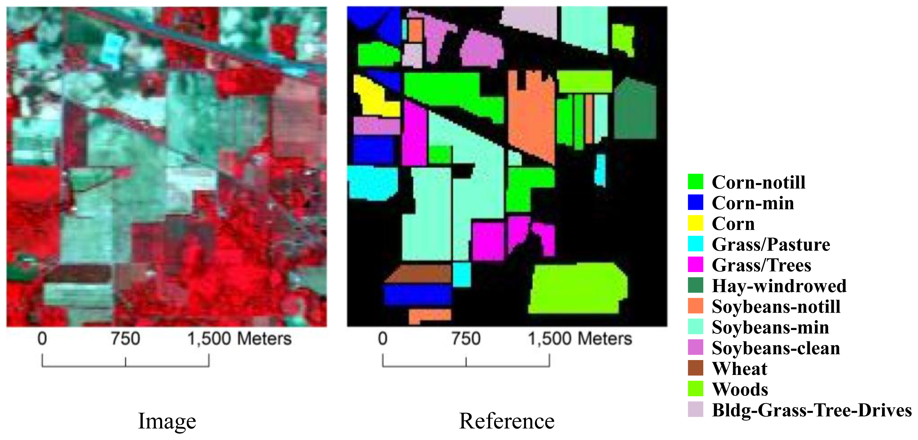
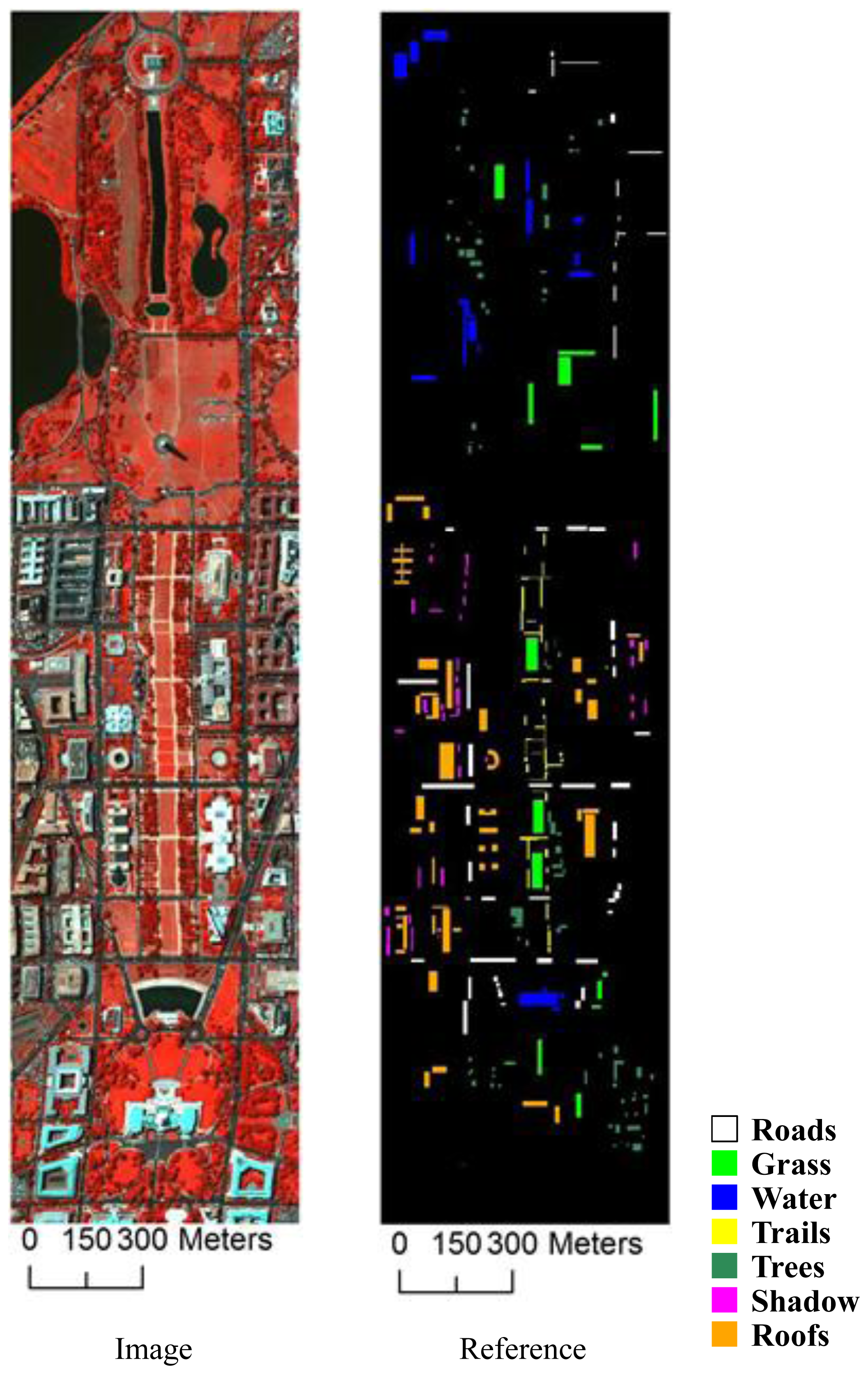
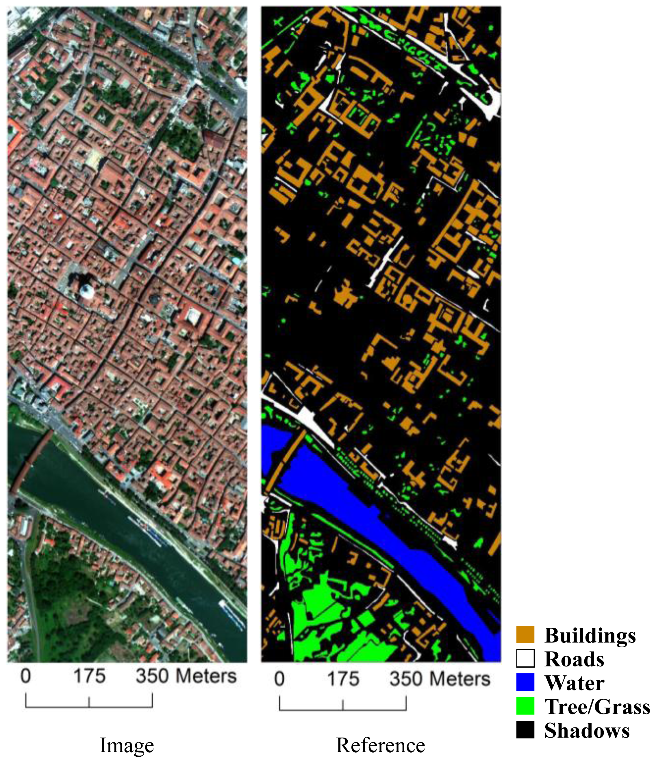
In our experiments, the proposed MCH feature is evaluated with four hyperspectral datasets. The first dataset is the AVIRIS (Airborne Visible/Infrared Imaging Spectrometer) image from the Indian Pines test site, containing 145 × 145 pixels with 220 bands [26]. The second dataset was collected by the HYDICE (Hyperspectral Digital Imagery Collection Experiment) sensor over the Mall, Washington DC. This image contains 1280 × 307 pixels with 191 bands [26]. The other two datasets were collected by the ROSIS (Reflective Optics System Imaging Spectrometer) sensor over the city center and University of Pavia, central Italy. After removal of the noisy bands, the image of Pavia University is of a size of 610 × 340 with 103 bands, and the image of Pavia City has 102 bands with 1400 × 512 pixels [27]. These data sets are widely used for assessing model validity. Note that the images are provided without atmospheric correction, which is similar to the current literature where the same data sets are used [5,10,14,28]. The images and the corresponding reference data are presented in Figures 3–6 for the Indian Pines, Washington DC, Pavia University, and Pavia City datasets, respectively. Meanwhile, the samples for the datasets are reported in

Table 1. Numbers of samples for the Indian Pines image.

Class	# Training Samples	# Test Samples
Corn-notill	50	1434
Corn-mintill	50	834
Corn	50	234
Grass/pasture	50	497
Grass/trees	50	747
Hay-windrowed	50	489
Soybeans-notill	50	968
Soybeans-mintill	50	2468
Soybeans-cleantill	50	614
Wheat	50	212
Woods	50	1294
Bldg-Grass-Tree-Drives	50	380
Total	600	10,171

Table 2. Numbers of samples for the Washington DC image.

Class	# Training Samples	# Test Samples
Roads	50	3299
Grass	50	3075
Water	50	2882
Trails	50	1017
Trees	50	2027
Shadows	50	1093
Roofs	50	5811
Total	350	19,024

Table 3. Numbers of samples for the Pavia University image.

Class	# Training Samples	# Test Samples
Trees	50	3064
Asphalt	50	6631
Bitumen	50	1330
Gravel	50	2099
Metal sheets	50	1345
Shadows	50	947
Bricks	50	3682
Meadows	50	18,649
Bare soil	50	5029
Total	450	42,776

–

Table 4. Numbers of samples for the Pavia City image.

Class	#Training Samples	# Test Samples
Buildings	50	84,421
Roads	50	18,149
Water	50	38,875
Trees/grass	50	40,630
Shadows	50	12,532
Total	250	194,607

.

3.2. Parameter Analysis

In this subsection, the experimental results are analyzed with different numbers of clusters and sizes of windows. A set of values for these parameters is selected according to the spatial resolution and the characteristics of the classes in the image, in order to investigate their influence on the proposed MCH method. The Indian Pines image and the Pavia University image, with k-means clustering, are used for the parameter analysis.

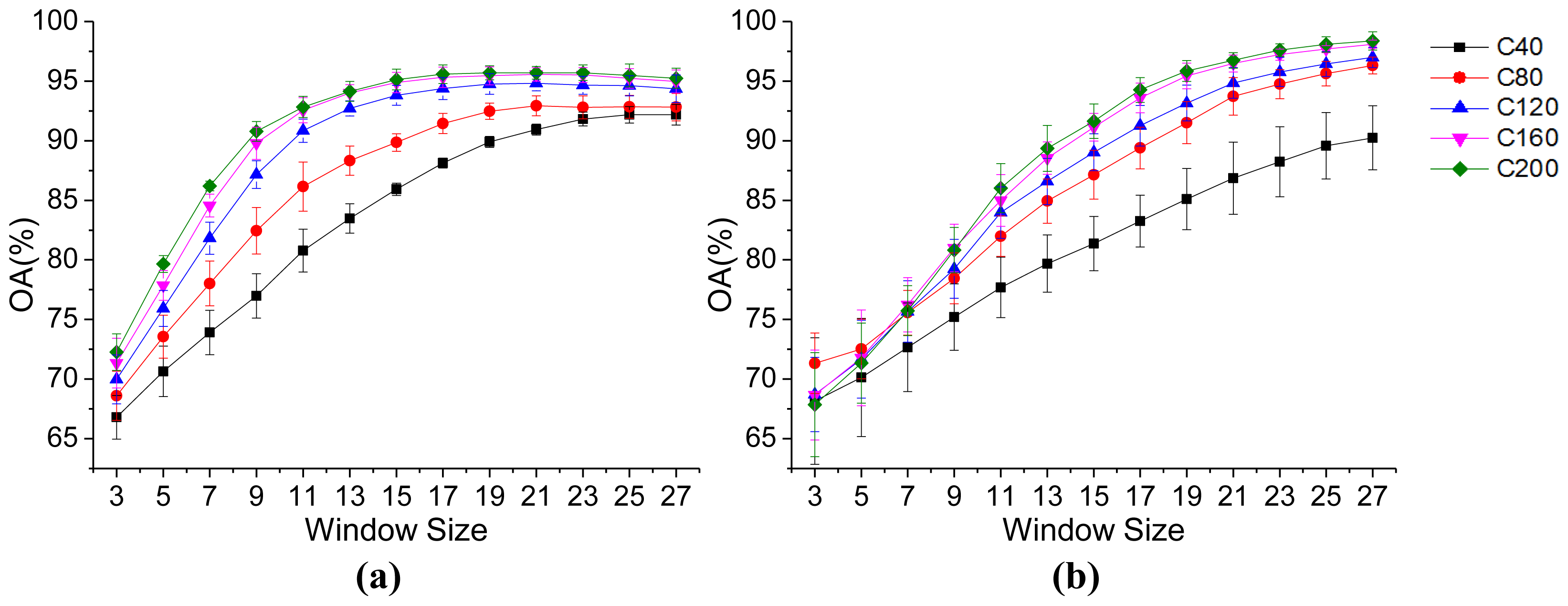
In Figure 7, the overall accuracies achieved with different cluster numbers and window sizes are presented. For both the Indian Pines image (Figure 7a) and the Pavia University image (Figure 7b), the algorithm with 200 clusters achieves the best performance, and the worst results are produced with 40 clusters. Meanwhile, the accuracy with 160 clusters is very similar to the optimal result. It can be seen that when the number of clusters exceeds a certain threshold, the performance of the proposed algorithm becomes more stable and the deviation in the accuracy is less. On the other hand, the overall accuracy rises rapidly with the increase in the window size. When the window size reaches a certain size, however, the rising trend slows down, especially for a larger cluster number.

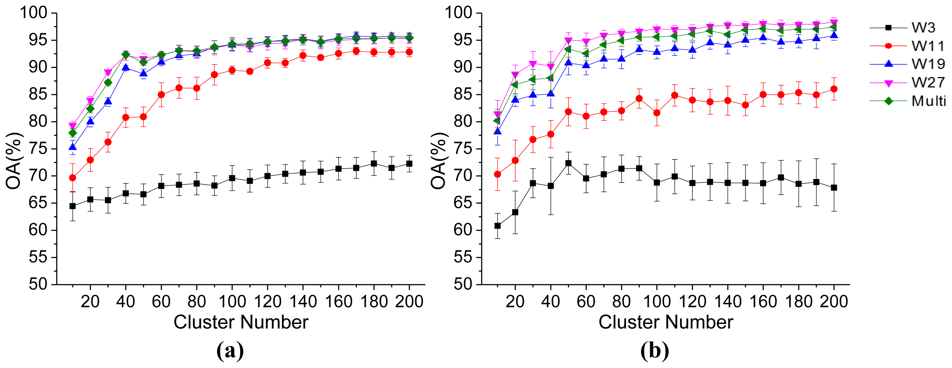
Meanwhile, the multiscale approach is compared to a single-scale (or single-window) method. As shown in Figure 8a, the accuracies given by the MCH are similar to the best results achieved by the single-scale approach for the Indian Pines image. As for the Pavia University image (see Figure 8b), the accuracies given by the multiscale approach are a little lower than the optimal single-scale approach corresponding to a window size of 27, but are much better than the other cases. It is revealed that the multiscale histogram can provide a result that is close to the best performance of the single-window approach. This means that the use of the multiscale method can lead to an improved accuracy and avoids the selection of the optimal window size.

3.3. Results and Comparisons

To test the effectiveness of the proposed method, raw classification (i.e., classification using only the spectral bands) and several other spectral-spatial classification methods are carried out for comparison. The conventional spatial features considered for the comparison include the 3D wavelet texture, the GLCM, and DMPs.

3.3.1. 3D Wavelet Texture

The 3D wavelet transformation views the hyperspectral imagery as a cube and decomposes it into eight sub-bands {L^xL^yL^z, L^xH^yL^z, L^xL^yH^z, L^xH^yH^z, H^xL^yL^z, H^xH^yL^z, H^xL^yH^z, H^xH^yH^z}, where L and H represent the low-pass and high-pass sub-bands, respectively. x and y are the spatial coordinates of the image, and z is the spectral band [28]. These sub-bands are stacked with the original spectral bands as the input feature for the spectral-spatial classification. In this study, the parameters of the 3D wavelet texture are set as: window size = {4, 8, 16, 32}.

3.3.2. GLCM

The GLCM describes the distribution of co-occurring values at a given offset over a window of a specific size. In this study, contrast is used as the textural measure to complement the spectral signals for classification, as suggested in [29]. Meanwhile, to reduce the computational complexity, principal component analysis (PCA) is used to reduce the dimensionality of the spectral information, and the PCA transformations are used as the base images for the subsequent GLCM texture extraction. The parameters are set as: basis image = {PC1, PC2, PC3, PC4}, window size = {3, 7, 11, …, 27}, and direction = {0°, 45°, 90°, 135°}.

3.3.3. DMPs

Based on the mathematical morphology, DMPs are an effective structural feature extraction method when describing the shape profiles of objects at different scales [30]. DMPs are generated by using a composition of geodesic morphological operations with a set of structural elements. The DMPs and the spectral feature are then combined and input into the classifier for the spectral-spatial classification. Similarly, the PCA transformations are used as the base images for calculating the DMPs. The parameters of the DMPs are set as: basis image = {PC1, PC2, PC3, PC4}, radius of the disk structural element = {3, 6, 9, 12, 15}, morphological operation = {opening/closing by reconstruction}.

In order to evaluate the classification performance, the accuracy assessment is obtained by measuring the difference between the classification map and the reference data that represents the ground truth. The overall accuracy (OA) and kappa coefficient (kappa) are widely used accuracy assessment measures. The OA is generated by dividing the total number of correct predictions by the total number of samples in the reference data. The kappa coefficient is a more robust measure than OA, since kappa takes both the omission and commission errors into consideration. As for the accuracies of the specific classes, the producer’s and the user’s accuracy are used. The producer’s accuracy is a reference-based accuracy which represents the probability of reference samples being correctly classified, and the user’s accuracy is a map-based accuracy which indicates the probability that a pixel classified in the map actually represents the class on the ground [31]. In this paper, the F-score [32] is employed to integrate the producer’s accuracy and user’s accuracy:

$$F=\frac{2·PA·UA}{PA+UA}$$

(9)

where PA is the producer’s accuracy, and UA is the user’s accuracy.

In this paper, the parameters of the SVM are set as: penalty coefficient C = 100; kernel = RBF (radial basis function); and bandwidth of RBF = 1/d, where d is the dimension of the input features. Meanwhile, the OA, kappa coefficient, and F-score are used to assess the classification performance. In addition, all of the experimental results are reported with the optimal parameter values. The dimensions of the spatial feature are 8, 16, and 40 for the 3D wavelet texture, GLCM and DMP, respectively. Furthermore, the classification results of the whole image are presented for an overall visual inspection of the methods.

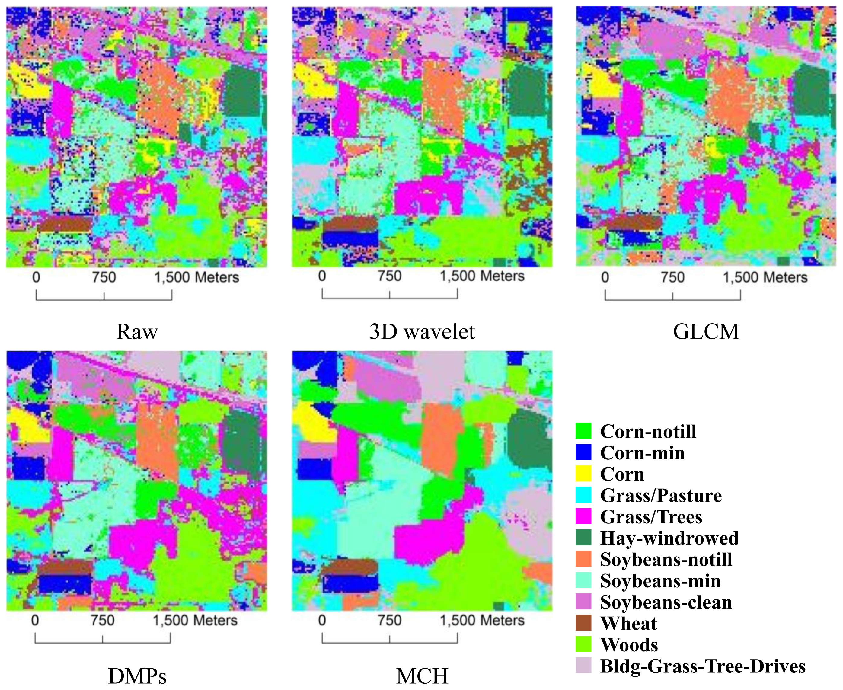
For the Indian Pines image, the spectral-spatial approaches significantly improve the classification accuracy (see Figure 9). From

Table 5. Classification accuracies of the different features for the Indian Pines image.

	Spectral-Spatial Classification				MCH
	Raw	3D Wavelet	GLCM	DMPs	k-Means	ISO	FCM	EM
Corn-notill	49.51	56.33	61.33	76.93	90.15	88.12	89.09	90.39
Corn-mintill	44.51	63.36	66.17	88.83	93.87	93.59	93.33	95.06
Corn	40.98	49.31	67.90	87.09	97.03	97.75	95.85	97.31
Grass/pasture	70.99	86.31	76.45	90.01	96.75	97.06	97.15	96.79
Grass/trees	82.27	90.90	91.08	94.71	99.44	99.68	99.67	99.57
Hay-windrowed	97.86	98.76	98.28	98.86	99.74	99.80	99.70	99.62
Soybeans-notill	55.51	60.28	62.15	76.17	89.89	87.98	88.86	90.14
Soybeans-mintill	57.17	65.02	67.28	88.32	95.08	95.05	94.98	95.15
Soybeans-cleantill	42.90	50.10	63.11	81.19	95.28	95.23	95.03	96.41
Wheat	87.82	96.75	98.52	99.35	99.72	99.81	99.72	99.67
Woods	86.47	93.60	91.63	98.73	99.91	99.92	99.92	99.90
Bldg-Grass-Tree-Drives	50.34	77.26	79.91	97.56	99.37	99.66	99.03	99.63
OA	61.83	70.73	73.40	88.08	95.34	94.90	95.00	95.60
kappa	0.57	0.67	0.70	0.86	0.95	0.94	0.94	0.95

, it is revealed that, compared to the spectral-only classification, the increases in the OAs given by the 3D wavelet texture, GLCM, and DMPs are 8.9%, 11.57%, and 26.25%, respectively. Even though these spatial features produce satisfactory results, the proposed MCH achieves much improved accuracies. The MCH with EM clustering shows the highest accuracy, OA = 95.6%, with an improvement on the primary result of 33.77%. Note that the accuracies obtained by the other clustering methods are all around 95%. On the other hand, all of the optimal class-specific accuracies are given by the MCH. In particular, for the corn-notill and soybeans-notill classes, the F-scores obtained by the other spatial features are less than 80%, but improved to 90.39% and 90.14% by the MCH method. Moreover, the F-scores of the classes given by the MCH are more than 90%, except for a couple of classes (corn-notill and soybeans-notill), and some class-specific accuracies are close to 100%.

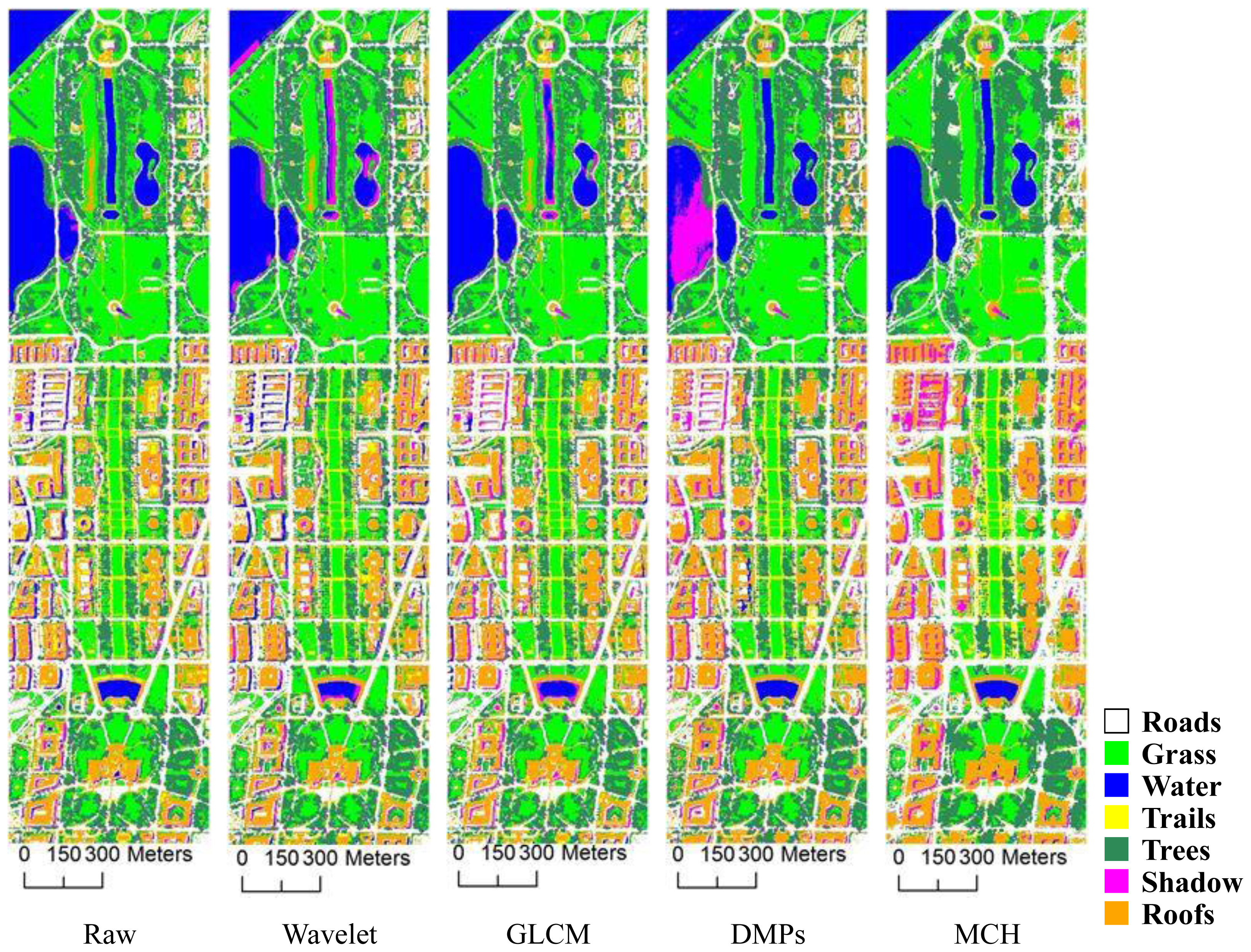
For the Washington DC image, the OA of the initial spectral-only classification is 86.61%, and the incorporation of the spatial information increases the accuracy by 5.67%, 8.19%, and 10.14%, corresponding to the 3D wavelet texture, GLCM, and DMPs, respectively (see

Table 6. Classification accuracies of the different features for the Washington DC image.

	Spectral-Spatial Classification				MCH
	Raw	3D Wavelet	GLCM	DMPs	k-Means	ISO	FCM	EM
Roads	91.70	91.79	92.04	95.37	98.98	98.87	98.81	98.84
Grass	98.85	99.32	99.22	99.72	99.86	99.84	99.86	99.76
Water	86.28	88.33	96.86	96.05	98.71	100.00	99.30	99.94
Trails	66.10	90.94	90.42	97.02	99.64	99.63	99.61	99.44
Trees	98.17	98.69	98.33	99.02	99.92	99.92	99.90	99.70
Shadows	39.93	67.70	90.53	90.17	96.86	99.63	97.77	99.50
Roofs	84.28	93.45	93.44	96.90	99.51	99.42	99.46	99.38
OA	86.61	92.28	94.80	96.75	99.24	99.55	99.34	99.48
kappa	0.84	0.91	0.94	0.96	0.99	0.99	0.99	0.99

). Meanwhile, the accuracies acquired by the MCH with the different clustering methods are all over 99%. With the MCH derived from the ISODATA clustering, the F-score of the shadows class increases from 39.93% to 99.60%, and the accuracies of water, trails, and roofs are also significantly enhanced. Furthermore, six specific classes obtain accuracies of over 99%. From a visual inspection (see Figure 10), the classification map given by the MCH shows a promising performance for the roofs, roads, and shadow classes.

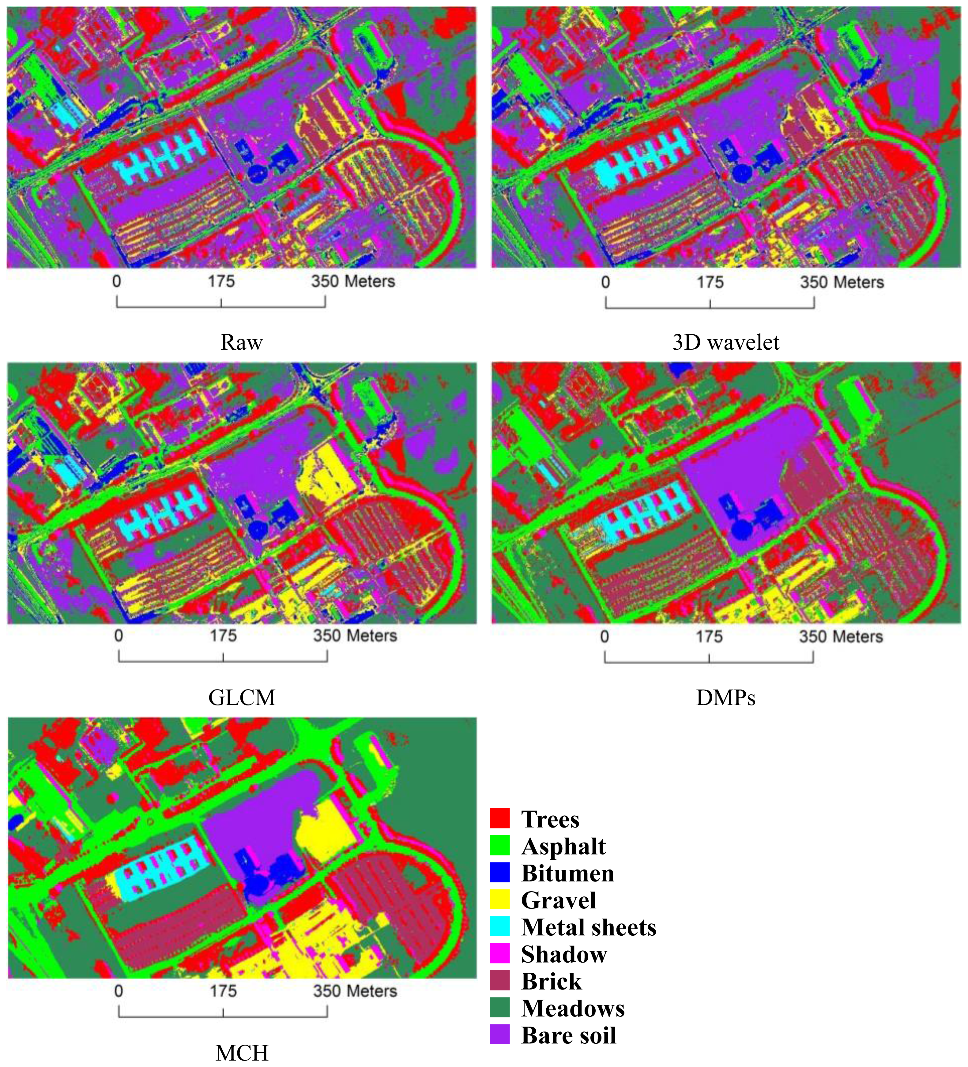
For the Pavia University image, as presented in

Table 7. Classification accuracies of the different features for the Pavia University image.

	Spectral-Spatial Classification				MCH
	Raw	3D Wavelet	GLCM	DMPs	k-Means	ISO	FCM	EM
Trees	62.85	63.22	70.95	87.03	97.70	97.77	97.29	97.50
Asphalt	77.94	80.60	78.81	96.16	97.99	97.90	96.86	99.59
Bitumen	49.65	56.06	59.14	99.86	99.29	99.81	96.69	100.00
Gravel	34.48	46.42	40.04	96.00	95.94	95.51	94.67	99.73
Metal sheets	91.00	93.99	92.72	99.71	99.93	99.88	99.83	99.93
Shadows	99.36	99.41	99.42	99.89	99.92	99.93	99.93	99.95
Bricks	59.90	66.66	69.53	92.80	97.56	98.56	96.68	99.37
Meadows	61.98	63.90	68.12	97.07	98.25	98.75	97.78	99.60
Bare soil	31.97	33.89	39.04	99.35	95.17	96.85	94.34	99.99
OA	59.42	62.67	64.84	96.18	97.73	98.23	97.00	99.51
kappa	0.50	0.54	0.57	0.95	0.97	0.98	0.96	0.99

and Figure 11, the classification with DMPs (OA = 96.18%) gives much better results than the other spatial features. Meanwhile, the OAs of the MCH with k-means, ISODATA, and FCM are 97.73%, 98.23%, and 97.00%, respectively, which is an obvious improvement over the DMPs. Furthermore, in this experiment, it is found that the MCH with EM clustering provides much better results (OA = 99.51%) than the other clustering methods. Additionally, the MCH with EM clustering improves the spectral classification from 63.63% to 99.51%. As for the class-specific accuracies, the F-scores are 66.4%, 53.25%, 46.37%, and 35.42% for gravel, bare soil, bitumen, and meadows, respectively.

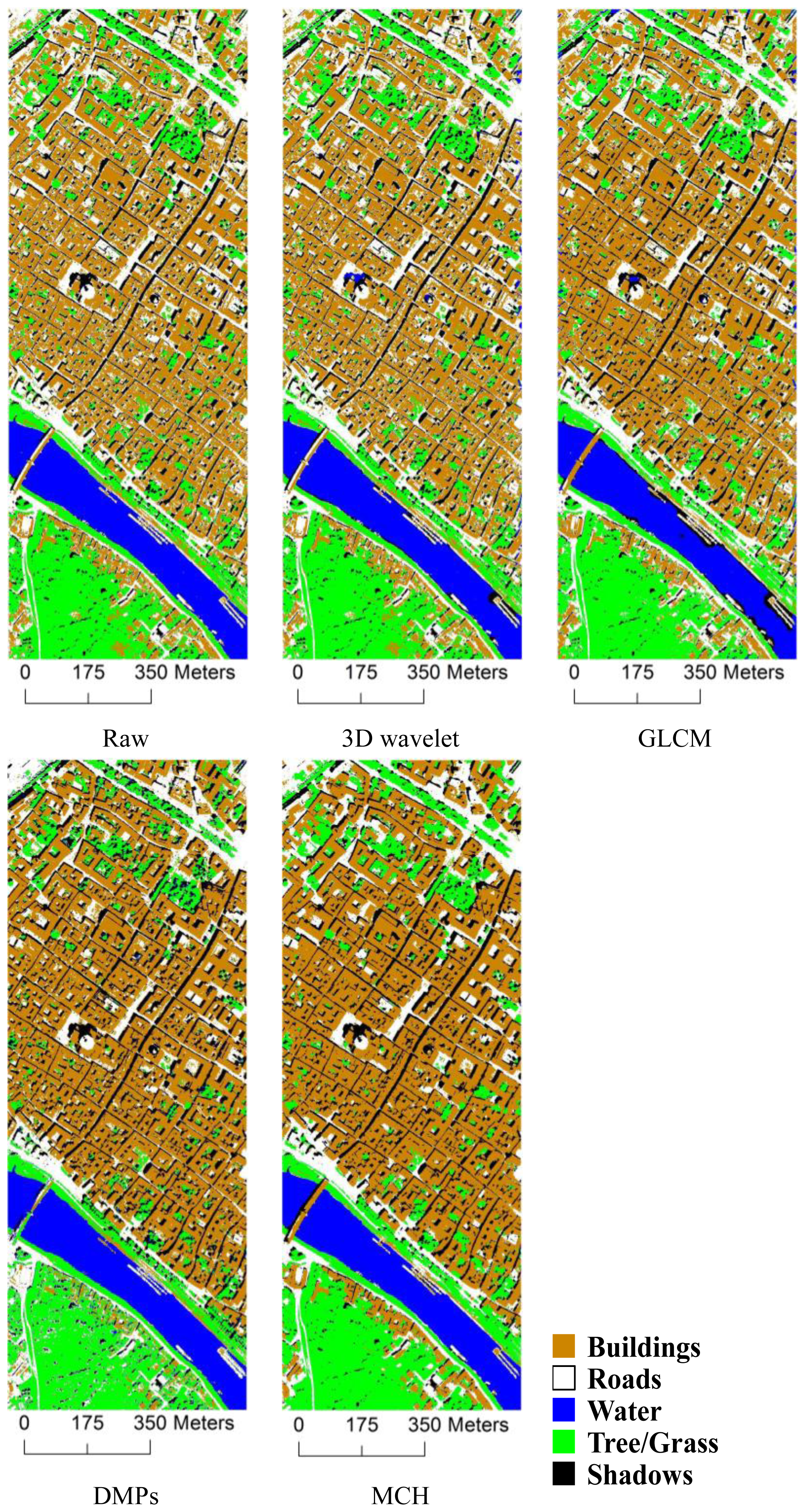
From

Table 8. Classification accuracies of the different features for the Pavia City image.

	Spectral-Spatial Classification				MCH
	Raw	3D Wavelet	GLCM	DMPs	k-Means	ISO	FCM	EM
Buildings	88.47	88.79	90.82	90.07	93.27	93.58	93.54	92.75
Roads	67.41	67.92	70.92	71.95	77.69	78.63	78.38	76.42
Water	99.61	98.92	98.79	99.34	99.99	99.94	99.98	99.86
Trees/grass	97.16	97.29	98.35	96.30	99.32	99.26	99.12	99.21
Shadows	95.43	93.82	93.12	91.34	95.95	95.30	96.03	94.71
OA	90.21	90.21	91.68	91.07	94.26	94.45	94.43	93.75
kappa	0.87	0.87	0.89	0.88	0.92	0.92	0.92	0.91

, it can be seen that the increases in the accuracies achieved by the conventional spatial features are not significant for the Pavia City image. The result achieved with the GLCM, which is the best among the classical features, improves the spectral classification by only 0.86%. In addition, the accuracy obtained by the 3D wavelet texture is the same as the original classification. Whereas, when using the MCH, the improvements are 4.05%, 4.24%, 4.22%, and 3.54% with k-means, ISODATA, FCM, and EM clustering, compared to the spectral classification, respectively. As for the class-specific accuracies, almost all of the best results are given by the MCH with k-means and ISODATA. Overall, the MCH shows a remarkable improvement with spectrally similar classes, such as buildings and roads (see Figure 12).

3.4. Discussion

The MCH utilizes the distribution of the clusters in a local area as the spatial information for the spectral-spatial classification of hyperspectral imagery. Three further issues are now analyzed and discussed.

(1)

Dimensionality of the hyperspectral bands. The Indian Pines image is taken as an example for investigating the effect of the spectral dimensionality for the MCH method. The dimensions of the spectral features used for the clustering are reduced to 10, 30, and 50, according to Equation (4). From

Table 9. Classification accuracies for the Indian Pines image with different spectral dimensions for clustering.

Dim.	k-Means		ISO		FCM		EM
	Mean	Std.	Mean	Std.	Mean	Std.	Mean	Std.
10	95.34	0.98	94.90	0.89	95.00	0.98	95.60	0.94
30	95.28	1.09	95.23	0.73	95.06	1.00	95.65	1.17
50	95.28	1.08	95.10	0.87	95.15	1.09	95.56	0.90
All	95.46	0.89	95.14	0.87	94.74	0.93	95.40	0.84

, it can be seen that the spectral dimension of the clustering has little effect on the final classification accuracy. It is therefore sensible to appropriately reduce the spectral dimensionality in order to increase the efficiency of the MCH method, since the computational complexity of clustering is affected by the feature dimensionality.

(2)

Initialization of the clustering. To analyze the influence of initialization of the clustering on the classification, the accuracies with different initial clustering centers that are randomly generated are reported in

Table 10. Classification accuracies for the Indian Pines image with different clustering initializations.

Run		1	2	3	4	5	6	7	8	9	10
k-means	Mean	95.65	95.53	94.94	95.22	95.62	95.26	95.28	95.26	94.96	95.29
	Std.	0.67	0.93	1.10	0.88	0.77	1.02	0.98	0.82	0.95	0.80
FCM	Mean	95.44	95.17	95.31	95.29	95.09	95.27	95.07	95.29	95.18	95.55
	Std.	1.03	1.01	0.98	0.90	0.94	1.00	0.97	1.12	1.00	0.97
EM	Mean	95.62	95.65	95.18	95.77	95.98	95.43	95.62	95.87	95.51	95.81
	Std.	0.80	0.60	1.04	0.95	0.65	1.00	0.73	0.39	0.70	0.89

for the Indian Pines image. It can be seen that, although the clustering approach gives slightly different clustering results for the different runs, the classification accuracies are stable and the proposed MCH is robust to the clustering initialization.

(3)

Comparison with a state-of-the-art spectral-spatial classification technique. In order to further validate the effectiveness of the proposed MCH method, the state-of-the-art spectral-spatial classification approach of Tarabalka et al. [10] is carried out for comparison. In this approach, the pixelwise SVM classification result is refined by majority voting based on a clustering-based segmentation. A post-processing is then performed in order to reduce the classification noise. The comparison results are shown in

Table 11. Comparison between MCH and the state-of-the art spectral-spatial classification technique of Tarabalka et al. [10] (PP = post-processing for reducing the classification noise).

Datasets	MCH				Tarabalka et al. [10]
	k-Means	ISO	FCM	EM	Without PP	With PP
University	97.73	98.23	97.00	99.51	90.57	91.20
AVIRIS	95.34	94.90	95.00	95.60	88.53	90.64

, where it can be clearly seen that the MCH method significantly outperforms the state-of-the-art spectral-spatial classification approach of Tarabalka et al. [10].

A possible uncertainty is related to the atmospheric correction, which is not performed on the datasets since these images are widely used to investigate the effectiveness of algorithms in the remote sensing community. Nevertheless, the atmospheric correction is a standard practice which may have important impacts on the classification results. Consequently, different atmospheric correction methods can be applied to analyze their effect on the classification performance in the future research. Another limitation of the proposed method is that the MCH space is sparse when the number of the pixels within the local window is far less than the number of clusters. Therefore, the sparse representation methods can be considered for the image classification in the future.

4. Conclusions

In this paper, a novel multiscale cluster histogram (MCH) is proposed for the feature extraction and classification of hyperspectral images. On the one hand, the clustering algorithm partitions the pixels into a set of groups according to their feature similarity, which can be viewed as processing that makes use of the global characteristics. On the other hand, the spatial feature is then extracted based on a set of windows, which represents the local structures. Consequently, the proposed MCH is actually a joint global-local spatial feature extraction method. The proposed method has the following characteristics:

(1)

The clustering strategy is able to generate a series of primitive codes which effectively represent the spectral signals in an image.

(2)

The cluster histogram in a series of multiscale neighborhoods centered by each pixel is effective in exploiting both the spectral and spatial features. Furthermore, the multi-window strategy assigns large weights to the pixels near the center, which is reasonable due to the complex and multiscale characteristics of the remote sensing data.

(3)

The MCH feature extraction and classification method can achieve satisfactory results rapidly and conveniently without defining complicated textural or structural features. It can also be easily carried out in real applications.

The experiments verify that the proposed algorithm significantly improves the spectral classification result, and, in particular, it is proved to be highly suitable for hyperspectral image classification. With the four widely used hyperspectral datasets, the MCH presents an outstanding performance. For instance, the EM-based MCH achieves 95.6%, 99.5%, 99.5%, and 93.8% for OA in the Indian Pines, Washington DC, Pavia University, and Pavia city data sets, respectively. Furthermore, MCH significantly outperforms other commonly used spatial features (e.g., GLCM (gray-level co-occurrence matrix), DMPs (Differential Morphological Profiles), and 3D wavelet). Based on the analysis and comparison, it can be seen that the MCH-based hyperspectral image classification is robust to the feature dimension and clustering initialization. Possible directions of future research are the similarity measures for hyperspectral data [33], and the use of clustering algorithms such as CLARA [34] for the rapid implementation of the clustering.

Generally speaking, the proposed MCH method is effective for representing hyperspectral imagery and provides excellent classification accuracies. The computation time for the proposed MCH is actually related to the clustering, which is fast and easy to implement. The property shows that the MCH has the potential to be a practical algorithm for processing images with large areas. We believe that it could be conveniently applied in real applications as one of the standard classification tools.

References

1. Pal, M.; Mather, P.M. An assessment of the effectiveness of decision tree methods for land cover classification. Remote Sens. Environ 2003, 86, 554–565. [Google Scholar]
2. Melgani, F.; Bruzzone, L. Classification of hyperspectral remote sensing images with support vector machines. IEEE Trans. Geosci. Remote Sens 2004, 42, 1778–1790. [Google Scholar]
3. Gong, B.; Im, J.; Mountrakis, G. An artificial immune network approach to multi-sensor land use/land cover classification. Remote Sens. Environ 2011, 115, 600–614. [Google Scholar]
4. Myint, S.W.; Gober, P.; Brazel, A.; Grossman-Clarke, S.; Weng, Q. Perpixel vs. object-based classification of urban land cover extraction using high spatial resolution imagery. Remote Sens. Environ 2011, 115, 1145–1161. [Google Scholar]
5. Huang, X.; Zhang, L. An SVM ensemble approach combining spectral, structural, and semantic features for the classification of high-resolution remotely sensed imagery. IEEE Trans. Geosci. Remote Sens 2013, 51, 257–272. [Google Scholar]
6. Comaniciu, D.; Meer, P. Mean shift: A robust approach toward feature space analysis. IEEE Trans. Pattern Anal. Mach. Intell 2002, 24, 603–619. [Google Scholar]
7. Baatz, M.; Schäpe, A. Multiresolution segmentation: An optimization approach for high quality multi-scale image segmentation. Angew. Geogr. Inf 2000, 12, 12–23. [Google Scholar]
8. Vincent, L.; Soille, P. Watersheds in digital spaces: An efficient algorithm based on immersion simulations. IEEE Trans. Pattern Anal. Mach. Intell 1991, 13, 583–598. [Google Scholar]
9. Meinel, G.; Neubert, M. A comparison of segmentation programs for high resolution remote sensing data. Int. Arch. Photogramm. Remote Sens. Spat. Inf. Sci 2004, 35, 1097–1105. [Google Scholar]
10. Tarabalka, Y.; Benediktsson, J.A.; Chanussot, J. Spectral-spatial classification of hyperspectral imagery based on partitional clustering techniques. IEEE Trans. Geosci. Remote Sens 2009, 47, 2973–2987. [Google Scholar]
11. Baraldi, A.; Panniggiani, F. An investigation of the textural characteristics associated with gray level co-occurrence matrix statistical parameters. IEEE Trans. Geosci. Remote Sens 1995, 33, 293–304. [Google Scholar]
12. Benediktsson, J.A.; Pesaresi, M.; Arnason, K. Classification and feature extraction for remote sensing images from urban areas based on morphological transformations. IEEE Trans. Geosci. Remote Sens 2003, 41, 1940–1949. [Google Scholar]
13. Yoo, H.Y.; Lee, K.; Kwon, B.-D. Quantitative indices based on 3D discrete wavelet transform for urban complexity estimation using remotely sensed imagery. Int. J. Remote Sens 2009, 30, 6219–6239. [Google Scholar]
14. Tong, X.; Xie, H.; Weng, Q. Urban land cover classification with airborne hyperspectral data: What features to use? IEEE J. Sel. Top. Appl. Earth Observ. Remote Sens 2013. [Google Scholar] [CrossRef]
15. Zhang, L.; Huang, X.; Huang, B.; Li, P. A pixel shape index coupled with spectral information for classification of high spatial resolution remotely sensed imagery. IEEE Trans. Geosci. Remote Sens 2006, 44, 2950–2961. [Google Scholar]
16. Pedergnana, M.; Marpu, P.R.; Mura, M.D.; Benediktsson, J.A.; Bruzzone, L. Classification of remote sensing optical and LiDAR data using extended attribute profiles. IEEE J. Sel. Top. Signal Process 2012, 6, 856–865. [Google Scholar]
17. Gong, P.; Howarth, P.J. Frequency-based contextual classification and gray-level vector reduction for land-use identification. Photogramm. Eng. Remote Sens 1992, 58, 423–437. [Google Scholar]
18. Xu, B.; Gong, P.; Seto, E.; Spear, R. Comparison of gray-level reduction and different texture spectrum encoding methods for land-use classification using a panchromatic IKONOS image. Photogramm. Eng. Remote Sens 2003, 69, 529–536. [Google Scholar]
19. Jain, A.K.; Murty, M.N.; Flynn, P.J. Data clustering: A review. ACM Comput. Surv 1999, 31, 264–323. [Google Scholar]
20. MacQueen, J. Some Methods for Classification and Analysis of Multivariate Observations. In Proceedings of the Fifth Berkeley Symposium on Mathematical Statistics and Probability; University of California Press: Berkeley, CA, USA, 1967; Volume 1, pp. 281–297. [Google Scholar]
21. Ball, G.; Hall, D. ISODATA, A Novel Method of Data Analysis and Classification; Technical Report, AD–699616; Stanford University: Stanford, CA, USA, 1965. [Google Scholar]
22. Bezdek, J.C.; Ehrlich, R.; Full, W. FCM: The fuzzy c-means clustering algorithm. Comput. Geosci 1984, 10, 191–203. [Google Scholar]
23. Dempster, A.P.; Laird, N.M.; Rubin, D.B. Maximum likelihood from incomplete data via the EM algorithm. J. R. Stat. Soc. B 1977, 39, 1–38. [Google Scholar]
24. Huang, X.; Lu, Q.; Zhang, L. A multi-index learning approach for classification of high-resolution remotely sensed images over urban areas. ISPRS J. Photogramm. Remote Sens 2014, 90, 36–48. [Google Scholar]
25. Chang, C.-C.; Lin, C.-J. LIBSVM: A library for support vector machines. ACM Trans. Int. Syst. Technol 2011, 2, 1–27. [Google Scholar]
26. MultiSpec. Available online: Https://engineering.purdue.edu/~biehl/MultiSpec/hyperspectral.html (accessed on 20 October 2011).
27. Hyperspectral Remote Sensing Scenes. Available online: http://www.ehu.es/ccwintco/index.php/Hyperspectral_Remote_Sensing_Scene (accessed on 12 June 2013).
28. Ye, Z.; Prasad, S.; Li, W.; Fowler, J.E.; He, M. Classification based on 3-D DWT and decision fusion for hyperspectral image analysis. IEEE Geosci. Remote Sens. Lett 2014, 11, 173–177. [Google Scholar]
29. Pesaresi, M.; Gerhardinger, A.; Kayitakire, F. A robust built-up area presence index by anisotropic rotation-invariant textural measure. IEEE J. Sel. Top. Appl. Earth Observ. Remote Sens 2008, 1, 180–192. [Google Scholar]
30. Pesaresi, M.; Benediktsson, J.A. A new approach for the morphological segmentation of high-resolution satellite imagery. IEEE Trans. Geosci. Remote Sens 2001, 39, 309–320. [Google Scholar]
31. Congalton, R.G. A review of assessing the accuracy of classifications of remotely sensed data. Remote Sens. Environ 1991, 37, 35–46. [Google Scholar]
32. Powers, D.M.W. Evaluation: From Precision, Recall and F-measure to ROC, Informedness, Markedness & Correlation. J. Mach. Learn. Technol 2011, 2, 37–63. [Google Scholar]
33. Van der Meer, F. The effectiveness of spectral similarity measures for the analysis of hyperspectral imagery. Int. J. Appl. Earth Obs. Geoinf 2006, 8, 3–17. [Google Scholar]
34. Kaufman, L.; Rousseeuw, P.J. Clustering Large Applications (Program CLARA). In Finding Groups in Data: An Introduction to Cluster Analysis; John Wiley & Sons: New York, NY, USA, 1990. [Google Scholar]
Figure 1. Flowchart of the multiscale cluster histogram (MCH) algorithm.
Remotesensing 06 05732f1
Figure 2. Demonstration of the MCH (W is the local window, and H is the corresponding cluster histogram).
Remotesensing 06 05732f2
Figure 3. The Indian Pines image and its reference data.
Remotesensing 06 05732f3
Figure 4. The Washington DC image and its reference data.
Remotesensing 06 05732f4
Figure 5. The Pavia University image and its reference data.
Remotesensing 06 05732f5
Figure 6. The Pavia City image and its reference data.
Remotesensing 06 05732f6
Figure 7. Classification accuracies of the proposed algorithm with different cluster numbers (40, 80, 120, 160, 200) for: (a) the Indian Pines image; and (b) the Pavia University image.
Remotesensing 06 05732f7
Figure 8. Classification accuracies of the proposed algorithm with different window sizes (3, 11, 19, 27, and multiscale) for: (a) the Indian Pines image; and (b) the Pavia University image.
Remotesensing 06 05732f8
Figure 9. An overview of the classification maps for the Indian Pines image.
Remotesensing 06 05732f9
Figure 10. An overview of the classification maps for the Washington DC image.
Remotesensing 06 05732f10
Figure 11. An overview of the classification maps for the Pavia University image.
Remotesensing 06 05732f11
Figure 12. An overview of the classification maps for the Pavia City image.
Remotesensing 06 05732f12