A Multi-Scale Weighted Back Projection Imaging Technique for Ground Penetrating Radar Applications


Abstract
:1. Introduction
2. Multi-Scale Weighted Back Projection Algorithm
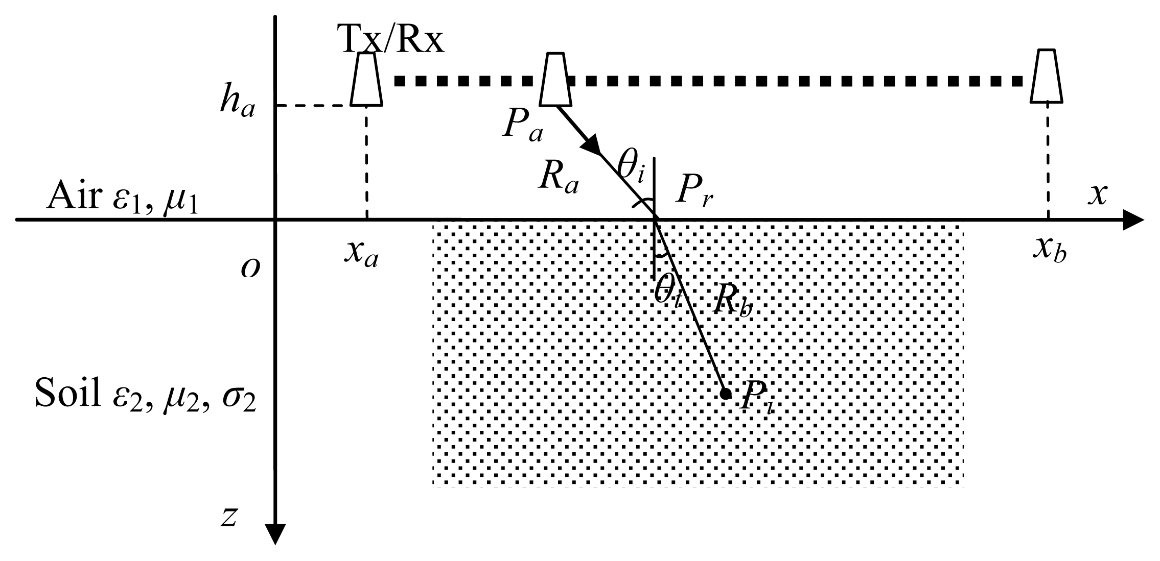
2.1. Traditional BP Imaging Algorithm
2.2. Multi-Scale Weighted BP Imaging Algorithm
2.2.1. Multi-Scale Processing
(1) Initial sampling grid
(2) PTR delination
(3) Hierarchical refinement coefficient
(4) Iteration stop condition
2.2.2. Weighted Factor
3. Experiments and Imaging Results
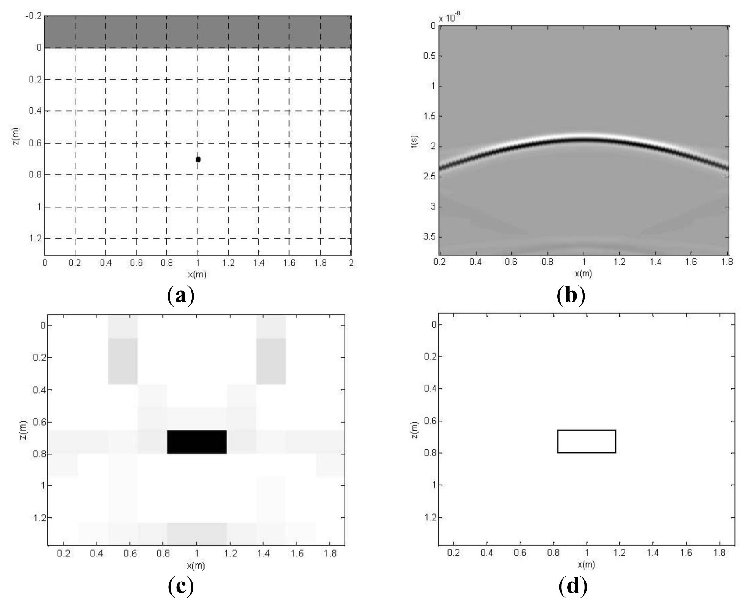
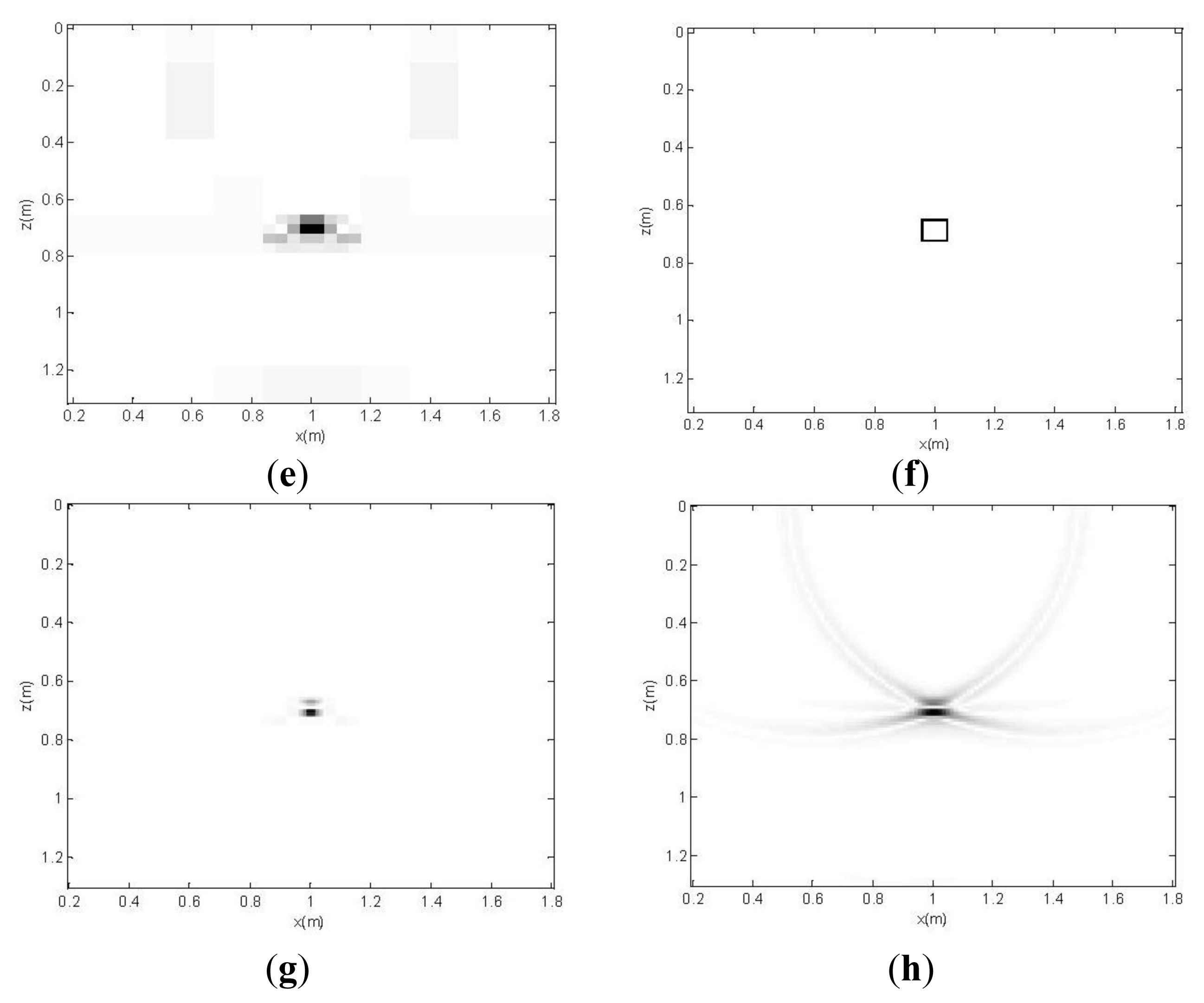
Example 1
Example 2
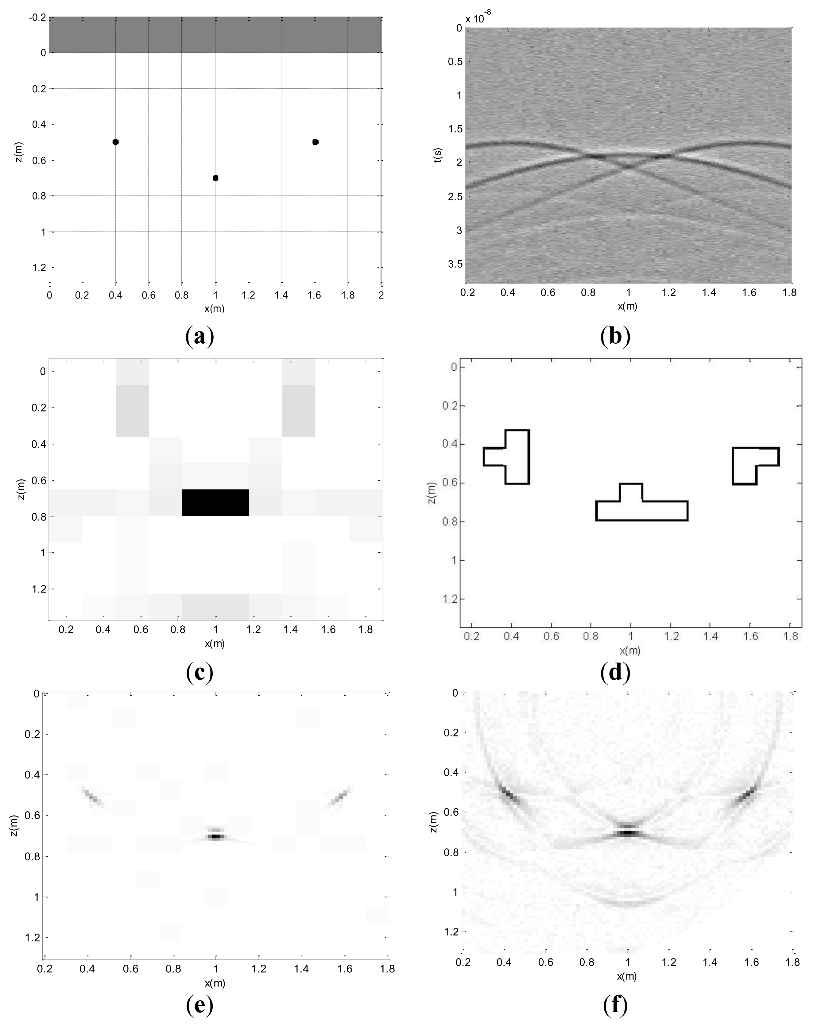
Example 3
4. Conclusions
Acknowledgments
Conflicts of Interest
- Author ContributionsWentai Lei presented the idea of multi-scale weighted BP imaging technique and carried out simulation experiments. Ronghua Shi carried out on-site GPR experiment and collected real GPR data. Jian Dong provided GPR simulation code and carried out GPR simulation based on FDTD technique. Yujia Shi carried out code implementation of multi-scale weighted BP imaging technique.
References
- Harry, M.J. NDT Transportation. In Ground Penetrating Radar Theory and Applications; Elsevier Science: Amsterdam, The Netherlands, 2009; pp. 20–30. [Google Scholar]
- Su, Y.; Huang, C.L.; Lei, W.T. Introduction. In Ground Penetrating Radar Theory and Applications; Science Press: Beijing, China, 2006; pp. 10–20. (In Chinese) [Google Scholar]
- Suksmono, A.B.; Bharata, E.; Lestari, A.A.; Yarovoy, A.G.; Ligthart, L.P. Compressive stepped-frequency continuous-wave ground-penetrating radar. IEEE Geosci. Remote Sens. Lett 2010, 7, 665–669. [Google Scholar]
- Gu, K.; Wang, G.; Li, J. Migration based SAR imaging for ground penetrating radar systems. IEE Proc. Radar Sonar Navig 2004, 151, 317–325. [Google Scholar]
- Eric, L.; Mill, R.; Willsky, A.S. Wavelet-based methods for the nonlinear inverse scattering problem using the extended Born approximation. Radio Sci 1996, 31, 51–65. [Google Scholar]
- Chiappinelli, P.; Crocco, L.; Isernia, T.; Pascazio, V. Multiresolution Techniques in Microwave Tomography and Subsurface Sensing. Proceedings of the International Geoscience and Remote Sensing Symposium, Congress Centrum Hamburg, Hamburg, Germany, 28 June–2 July 1999.
- Caorsi, S.; Donelli, M.; Franceschini, D.; Massa, A. A new methodology based on an iterative multiscaling for microwave imaging. IEEE Trans. Microw. Theory Technol 2003, 51, 1162–1173. [Google Scholar]
- Catapano, I.; Crocco, L.; Isernia, T. A simple two-dimensional inversion technique for imaging homogeneous targets in stratified media. Radio Sci 2004, 39. [Google Scholar] [CrossRef]
- Catapano, I.; Crocco, L.; D’Urso, M.; Isernia, T. On the effect of support estimation and of a new model in 2D inverse scattering problems. IEEE Trans. Antennas Propag 2007, 55, 1895–1899. [Google Scholar]
- Soldovieri, F.; Solimene, R.; Lo Monte, L.; Bavusi, M.; Loperte, A. Sparse reconstruction from GPR data with applications to rebar detection. IEEE Trans. Instrum. Meas 2011, 60, 1070–1079. [Google Scholar]
- Ahmad, F.; Amin, M. Compressive urban sensing. SPIE Newsroom 2012. [Google Scholar] [CrossRef]
- Lei, W.T.; Liu, L.Y.; Huang, C.L.; Su, Y. Subsurface Imaging of Buried Objects from FDTD Modeled Scattered Field. Proceedings of the 3rd International Conference on Computational Electromagnetics and Its Applications, Beijing, China, 1–4 November 2004.
- Zhou, L.; Huang, C.L.; Su, Y. A fast back-projection algorithm based on cross correlation for GPR imaging. IEEE Geosci. Remote Sens. Lett 2012, 9, 228–232. [Google Scholar]
- Lei, W.; Zeng, S.; Zhao, J.; Wang, Q.; Liu, J. An improved back projection imaging algorithm for subsurface target detection. Turk. J. Electr. Eng. Comput. Sci 2013, 21, 1820–1826. [Google Scholar]
- Sullivan, D.M. Two-Dimensional Simulation. In Electromagnetic Simulation Using the FDTD Method; Wiley-IEEE Press: New York, NY, USA, 2000; pp. 45–55. [Google Scholar]
- Wu, H.-S.; Barba, J. Minimum entropy restoration of star field images. IEEE Trans. Syst. Man Cybern 1998, 28, 227–231. [Google Scholar]


| GPR Scanning Parameters | P = 81 | Δx = 2 cm |
| 1st iteration | a1 = 8 | Δx1 = 16 cm |
| 2nd iteration | k2 = 0.4; a2 = 4 | Δx2 = 4 cm |
| 3rd iteration | k3 = 0.5; a3 = 3 | Δx3 = 1.33 cm |
| GPR Scanning Parameters | P = 81 | Δx = 2 cm |
| 1st iteration | a1 = 5.5 | Δx1 = 10.67 cm |
| 2nd iteration | k2 = 0.5; a2 = 6 | Δx2 = 1.78 cm |
| GPR Scanning Parameters | P = 101 | Δx = 3.45 cm |
| 1st iteration | a1 = 10 | Δx1 = 34.5 cm |
| 2nd iteration | k2 = 0.6; a2 = 3 | Δx2 = 11.5 cm |
| 3rd iteration | k3 = 0.6; a3 = 4 | Δx3 = 2.88 cm |
© 2014 by the authors; licensee MDPI, Basel, Switzerland This article is an open access article distributed under the terms and conditions of the Creative Commons Attribution license (http://creativecommons.org/licenses/by/3.0/).
Share and Cite
Lei, W.; Shi, R.; Dong, J.; Shi, Y. A Multi-Scale Weighted Back Projection Imaging Technique for Ground Penetrating Radar Applications. Remote Sens. 2014, 6, 5151-5163. https://doi.org/10.3390/rs6065151
Lei W, Shi R, Dong J, Shi Y. A Multi-Scale Weighted Back Projection Imaging Technique for Ground Penetrating Radar Applications. Remote Sensing. 2014; 6(6):5151-5163. https://doi.org/10.3390/rs6065151
Chicago/Turabian StyleLei, Wentai, Ronghua Shi, Jian Dong, and Yujia Shi. 2014. "A Multi-Scale Weighted Back Projection Imaging Technique for Ground Penetrating Radar Applications" Remote Sensing 6, no. 6: 5151-5163. https://doi.org/10.3390/rs6065151
APA StyleLei, W., Shi, R., Dong, J., & Shi, Y. (2014). A Multi-Scale Weighted Back Projection Imaging Technique for Ground Penetrating Radar Applications. Remote Sensing, 6(6), 5151-5163. https://doi.org/10.3390/rs6065151