1. Introduction
The strategic management of summer irrigated crops, both herbaceous and woody crops, has relevant agro-environmental repercussions, e.g., as a means of avoiding the excessive use and the depletion of water resources, decreasing the rate of growth of GHG emissions and adopting soil conservation practices to guarantee that the future demands of agriculture are met [
1]. To assist in the process of decision-making about the management of agricultural land or the implementation of agrarian actions, it is crucial to identify and monitor the distribution of crops at different spatial (parcel, county or region) scales every year. In many regions, this information is obtained regularly through farmer communications, which are subsequently partially checked in a program of ground visits to certain fields. This procedure is time-consuming, highly expensive and usually delivers inconsistent results because it generates reporting discrepancies and covers small areas or only very few accessible sampling fields [
2]. An alternative and truly viable procedure to conduct a cost-effective follow-up of the crop field evaluation across large areas is to use affordable satellite imagery, which could also provide consistent data for studies involving multiple sampling times.
For decades, many investigations have addressed the topic of crop discrimination via remote sensing through the use of various sources of satellite imagery, such as Landsat, QuickBird or Terra Advanced Spaceborne Thermal Emission and Reflection Radiometer (ASTER) [
3–
5]. In this topic, several authors have observed that information concerning variations in crop calendar, crop patterns, crop management techniques and parcel sizes shall be incorporated to the classifier algorithms for a successful result [
6,
7]. These variations can be derived from the textural, contextual or, in some cases, morphological features of the images [
3–
5]. However, conventional methods based only on spectral pixel information lack these features, which limits their application for crop discrimination, mainly in heterogeneous parcels with high spectral variability and mixed pixels (e.g., in woody crops) [
8]. Per-field classification can overcome these problems by merging adjacent pixels within each individual field into spectrally and spatially homogeneous objects created via a segmentation process and then classifying at the object level. This approach, known as object-based image analysis (OBIA), also incorporates the mentioned features to the classifier algorithm, which can lead to a drastic improvement of classification accuracy [
9]. Recently, Castillejo-González
et al. [
8] enhanced pixel-based classifications up to 22% by applying OBIA in mapping ten different land use classes with QuickBird satellite imagery. Another source of errors is due to the high spectral similarity among different crops with common development patterns and growth calendars, e.g., herbaceous ones such as tomato, corn, safflower or sunflower [
5]. In these cases, confusion problems might be overcome by using multisource data composed of new discriminating features and by applying powerful methods, such as machine learning models, that enhance classification outputs [
10].
One of the most widely studied fields of machine learning is undoubtedly supervised learning [
11]. This type of learning seeks to derive a function (or, generally, a model) that can identify the class to which new examples belong based on a pre-labeled training set. Basically, the model is a function which value depends on a set of parameters (coefficients for LR or weights for ANNs) and the input variables. These parameters are adjusted based on the training samples. Among others, the three most common tasks in supervised learning are binary classification, multi-class classification and regression. If the examples belong to only two categories, then the task is called binary classification. If there are multiple categories, then it is multi-class classification. Lastly, if the output value is a real number, the task is called regression. In contrast to this type of flat classification task, many important real-world classification problems are naturally cast as a hierarchical structure, in which the classes to be predicted are organized into a predefined hierarchy similar to a tree [
12]. The advantage of using this type of technique is two-fold: the combined classifiers explore information about parent-child class relationships present in the hierarchy and, if the number of classes is large, the classifiers obtained will be less affected by the increase in problem complexity. For a highly interesting review of various hierarchical classification techniques and applications, we refer the reader to Silla and Freitas [
13].
Among these models, nonparametric classifiers such as decision trees (DT), logistic regression (LR), artificial neural networks (ANN) and support vector machines (SVM) have been successfully used for remote-sensed image classification of agricultural landscapes because they can describe the intricate and complex nonlinear relationships that exist between canopy-level spectral information and crop conditions [
14–
17]. In this study, we evaluated the accuracy of the four cited methods for the identification and mapping of nine major summer crops from bi-temporal ASTER images captured in early and late summer in an agricultural region of California. MLP and SVM methods were selected as base classifiers given their popularity and their proven performance for pixel-based remote sensing problems [
15], although only a very few investigations have tested their efficiency for object-based image analysis [
16] or for a detailed classification of crop-fields. In a previous investigation over this region [
5], classifications from a conventional decision tree algorithm reported a substantial degree of confusion occurred between certain herbaceous crops (e.g., alfalfa and safflower, among others) during the summer season, due primarily to similarities in the growth stage and cropping pattern during the period when the demand for crop irrigation in this agricultural area is intense. Although some level of miss-classification might be acceptable for an agricultural inventory, a thematic map of higher accuracy is required for the precise estimation of the area of each individual crop, e.g., to obtain further estimates of costs and predictions of possible water restrictions in summer. Therefore, we quantified the efficiency of the cited machine learning methods, either as single classifiers or combined in a hierarchical classification, for enhancing classification outputs both at the group level (woody or herbaceous) and at the level of individual crops. A first-stage binary classifier was trained to differentiate woody from herbaceous ones, and two second-stage multiclass classifiers (one for each group) were used to determine the specific crop. The classifiers were built from spectral and textural features derived from an OBIA framework, which allowed quantify the influence of these features in the accuracy of the classified map. Finally, classification errors due to quantity disagreement and allocation disagreement [
18] as affected by the type of crop were discussed in terms of their influence for management of agricultural lands.
2. Materials and Methods
2.1. Studied Cropland Area
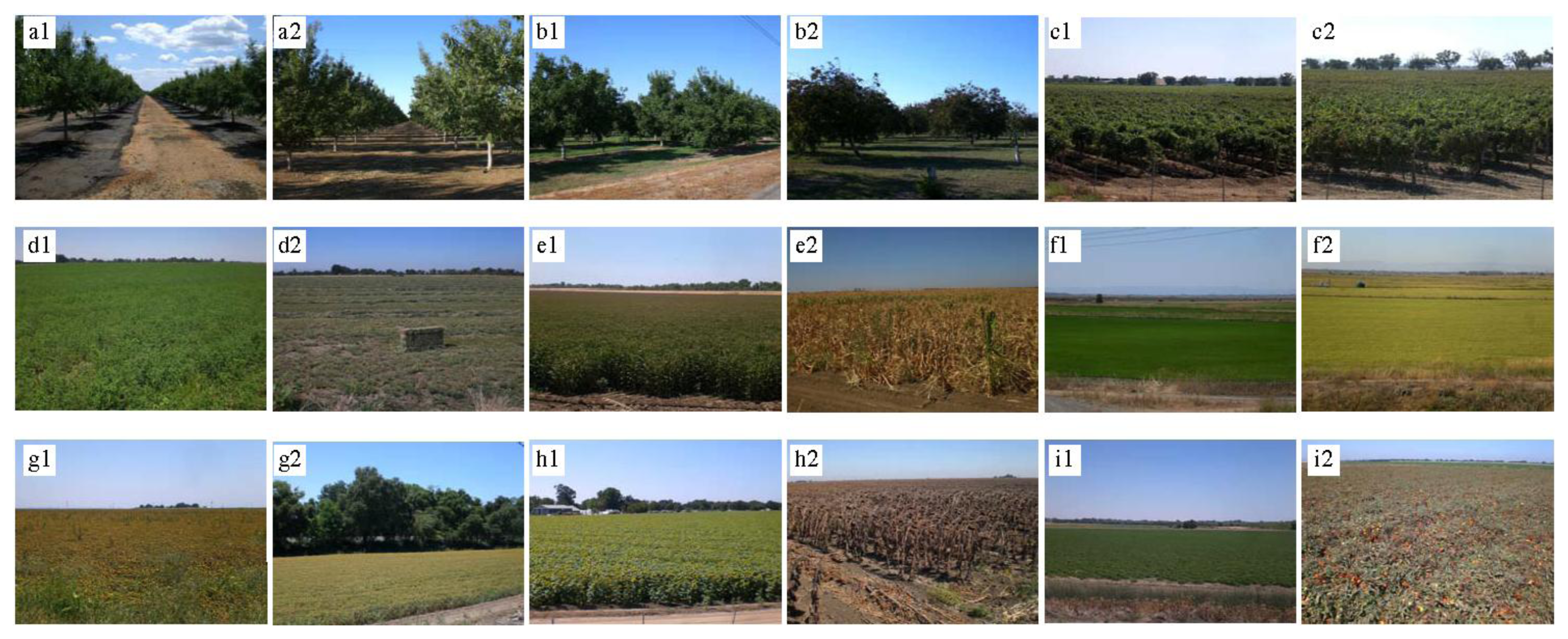
This investigation was conducted with nine major crops growing during the summer of 2006 in the agricultural region of Yolo County, California, USA (center lat/lon coordinates 38.50°N, 121.50°W). This region has a Mediterranean climate characterized by hot, dry summers (daily maximum temperatures greater than 38 °C) and cool winters (daily maximum temperatures of 16 °C). The rainfall ranges between 200 and 460 mm, with the key rainfall period between November and March. The irrigation infrastructure of the region consists of three dams, two reservoirs and more than 300 km of canals and ditches that use gravity to deliver the water. Various systems, such as spraying, dripping or flooding, are commonly used to irrigate the fields. Yolo County has a total agricultural surface area of 177,000 ha (out of a total county area of 264,900 ha) with a very diverse cropping pattern representative of agriculture in the Central Valley of California. Listed in order of total crop area, the woody crops included in this study were walnut (5%), vineyard (4%) and almond (3%), and the herbaceous crops were alfalfa (19%), tomato (14%), rice (10%), sunflower (6%), safflower (5%) and maize (4%). These crops covered 70% of the county’s cropland surface. The remaining 30% consisted of winter cereals (12%) and a combination of other types of hay and minor crops, for a total of as many as 130 different commodities. Apart from this cropland area, dry meadows represent approximately 20% of the county surface [
19].
Several differences in crop field patterns were observed during field visits due to the type of crop management operation conducted by each farmer. In woody crops, the field pattern was affected by the tree size, separation between trees, plantation design and use of cover crops. In herbaceous crops, two different systems were observed: (1) conservation systems, in which field soil is protected by maintaining residue from the previous crop; and (2) traditional systems, in which tillage operations remove residues and leave the soil surface bare. In alfalfa cultivation, vegetation permanently covers the soil, although its canopy density changes several times within a year according to its cutting schedule (between six and ten times a year). This intra-crop variability increases the complexity of crop discrimination, justifying the need to explore powerful algorithms for performing a robust classification adapted to different crop patterns. A general view of the studied crops during the summer is shown in
Figure 1.
2.2. Satellite Imagery and Derived Vegetation Indices
Based on a preliminary study of the crop calendars, we selected ASTER satellite images, obtained on 24 June and 12 September 2006, corresponding to key growth stages of the studied crops in early and late summer as previously reported by López-Granados
et al. [
20]. These authors successfully discriminated several types of crops at both extremes of the summer season by analyzing on-ground reflectance measurements. Either two or three scenes were acquired on each date to completely cover the studied zone. Each image was co-registered with ENVI 4.5 software (Research Systems Inc., Boulder, CO, USA) and then atmospherically corrected and radiometrically calibrated with its Fast Line-of-Site Atmospheric Analysis of Spectral Hypercubes (FLAASH) tool, which is based on MODTRAN4 radiative transfer code [
21]. This process is recommended in multi-temporal studies and it involves the conversion of the original raw digital values to reflectance values. The visible (green and red) and near-infrared (NIR) bands, with 15 m spatial resolution, and all six shortwave infrared (SWIR) bands, with 30 m spatial resolution, were combined by resampling the 30 m images to a 15 m pixel size with the nearest-neighbor method.
Differences in spectral reflectance can be enhanced through the use of vegetation indices (VIs). In this investigation, ten VIs derived from ASTER wavebands were calculated for both studied dates and grouped according to the spectral region to which they belong (
Table 1). The selected VIs have traditionally been used for monitoring variations in crop characteristics that can be crucial for discriminating summer crops [
22]. For example, the Normalized Difference VI (NDVI) and the Green VI (VIgreen) have commonly been used because they yield good relationships involving the type of vegetation, crop growth stage and assessment of crops [
23]. Other VIs based on the short-wave infrared (SWIR) region, such as the Normalized Difference Tillage Index (NDTI) or the Normalized Differential Senescent VI (NDSVI), have been defined to enhance information obtained in the senescent crop stage or from crop residues [
24]. The four studied machine learning models and the sixteen hierarchical configurations described in section 2.4 were constructed from an input dataset composed of the spectral VI described in
Table 1 [
23–
30].
2.3. Image Segmentation and Definition of Object-Based Textural Features
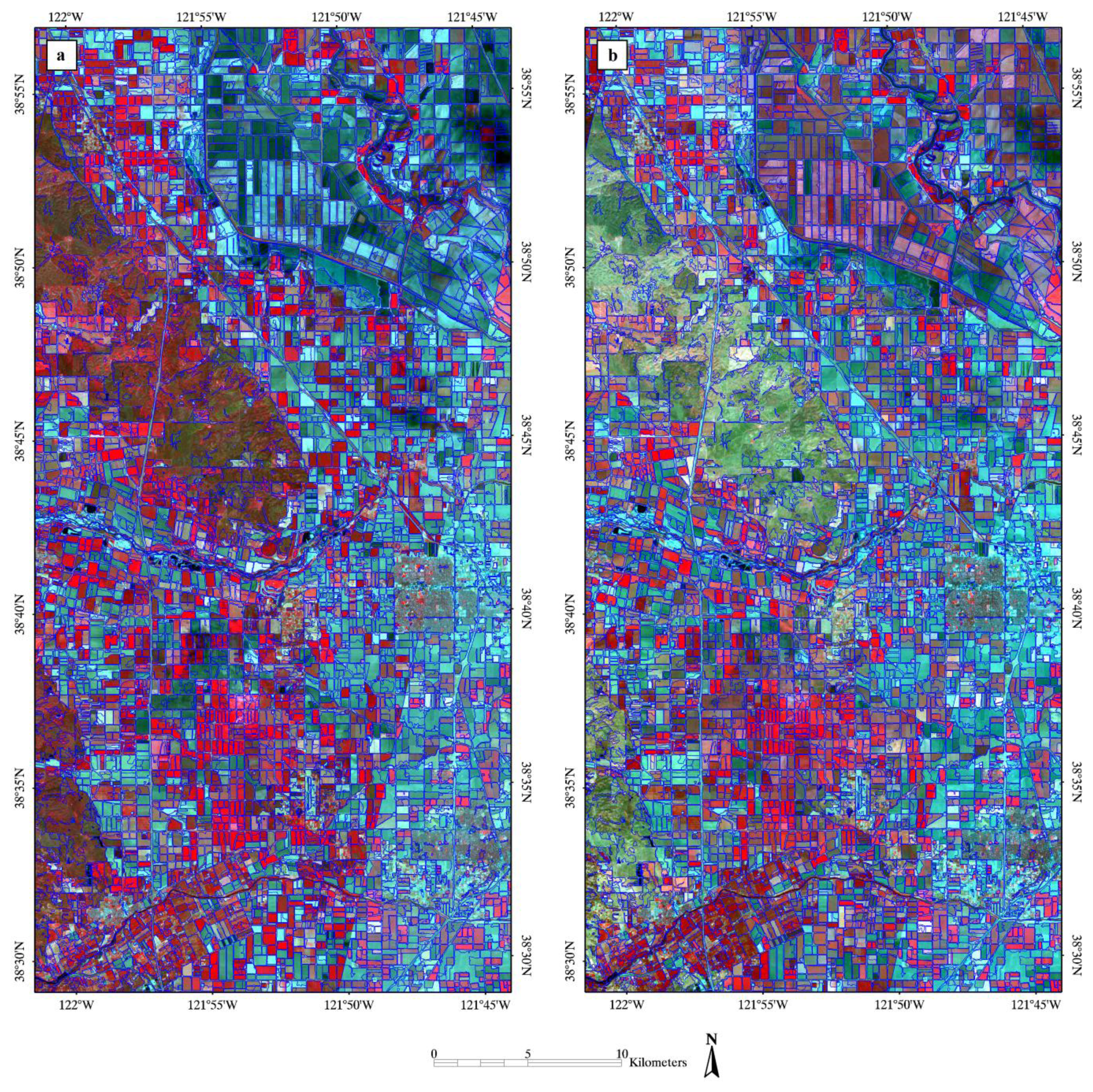
Two consecutive segmentation processes were applied to the satellite images to delimit the crop field borders and generate the object-based framework (
Figure 2). The multi-resolution segmentation algorithm implemented in the eCognition Developer 8 software (Trimble GeoSpatial, Munich, Germany) was used in both processes [
31] by equally weighting the Green, Red and NIR bands. Values of 0.4, 0.6, 0.2 and 0.8 for scale 50 and 0.9, 0.1, 0.3 and 0.7 for scale 100 were used for color, shape, smoothness and compactness, respectively. The geometric quality of the segmentation outputs was estimated by applying the empirical discrepancy method, which consisted on contrasting the segmentation output with an already computed ground-truth reference and quantifying their discrepancy measures based on differences among certain spatial features [
32]. In our investigation, we selected 350 ground-truth reference objects that represent fields from all the studied crop types and visually drew the field borders. Then, we assessed discrepancy in area, perimeter and shape index between the segmented objects and the real fields, reporting 94% average accuracy.
The object-based framework offers the possibility of computing the textural features that characterize each crop field. Object texture provides new information in addition to spectral data, and this information can enhance the power to discriminate heterogeneous classes [
33], although it has the disadvantage of higher computational cost. In this investigation, the following textural features were evaluated: (1) the standard deviation (SD) of the green, red and near-infrared wavebands and (2) the homogeneity, dissimilarity and entropy based on the gray-level co-occurrence matrix (GLCM) proposed by Haralick
et al. [
34]. The SD indicates the degree of local variability of the pixel values inside each object. The texture features based upon the GLCM were calculated by determining how often a pixel with the intensity (gray-level of the band considered) value i occurs in a specific spatial relationship to a pixel with the value
j [
31]. The homogeneity and dissimilarity features measure high or low object pixel uniformity, respectively, and the entropy feature is related to object pixel disorder [
35]. Because other textural features based on the GLCM are more complex to interpret in the context of cropland classification, they were excluded to reduce the computation time required by the analysis [
5].
2.4. Machine Learning Methods
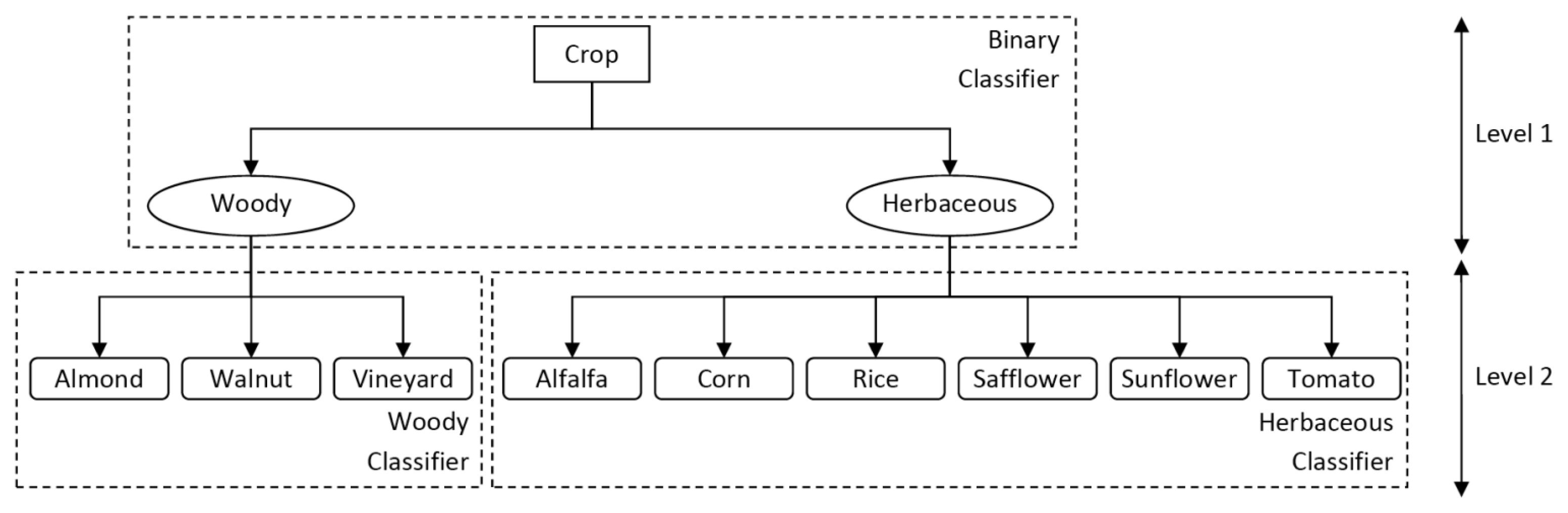
As previously discussed, a hierarchical classification technique was considered in order to count on the hierarchy information present in the target class variable,
i.e., the crop class. This hierarchy is shown in
Figure 3, distinguishing the classes for which each classifier was trained.
Two levels of classification were included:
- (1)
The first level was produced by a binary classifier, which was trained using the entire set of objects labeled as “woody” or “herbaceous”. The training dataset is described in Section 2.5.
- (2)
The second level was formed by two multi-class classifiers, one for each group of crops. Each classifier was trained using objects of the corresponding group (woody or herbaceous classifier). The labels for the three-class woody classifier were “almond”, “walnut” and “vineyard”, and the labels for the six-class herbaceous classifier were “alfalfa”, “corn”, “rice”, “safflower”, “sunflower” and “tomato”.
Once the three classifiers were obtained, the prediction was made by first applying the level-1 binary classifier to decide if the crop was woody or herbaceous and then using the corresponding specific level-2 classifier to decide a final class. To evaluate different configurations, four different types of algorithms were selected to construct level-1 and level-2 decision models, covering several of the most common machine learning classifiers:
- (1)
MultiLayer Perceptron (MLP): Artificial neural networks can associate complicated information with target attributes without any constraints on the sample distribution [
36]. MLPs are the most common choice and correspond to a functional model whose hidden units are sigmoidal basis functions. We used the implementation included in the Weka machine learning tool [
37], which applies a standard backpropagation process to optimize the different weights of the model. The number of hidden neurons,
h, was obtained from the heuristic
h = (
i +
c)/2, where i is the number of inputs and
c is the number of classes. The number of iterations,
i, was decided by a nested 5-fold cross-validation process, where
i takes values in the following range
i ∈{50,100,150,200,250,300}.
- (2)
Logistic Regression (LR): LR has become a widely used and accepted method of analysis for binary or multiclass outcome variables, as it can predict the probabilities associated with the states of the variables [
17]. Various algorithms can be applied to obtain the LR model. For this study, we selected the Simple Logistic algorithm included in Weka. The Simple Logistic algorithm builds multinomial logistic regression models with the LogitBoost algorithm (a boosting algorithm that performs forward stagewise fitting), first proposed by Friedman
et al. [
38] for fitting additive logistic regression models by maximum likelihood. The Simple Logistic algorithm adds one variable on each iteration, selecting the optimum number of iterations with a nested 5-fold cross-validation. This approach allows the pruning of certain inputs by stopping early in the analysis, thus avoiding overfitting.
- (3)
Support Vector Machine (SVM): It is a kernel learning method for classification problems in which linear separation is not possible in the input space [
39]. SVM operates a non-linear transformation of the original input space
X into a high dimensional feature space
F, where optimal separating hyperplanes can be found. This is done by using a reproducing kernel function which plays a key role in the final performance of the classifier. In this paper, we consider the most general choice, the Gaussian kernel function. The kernel width associated to the Gaussian,
σ, is adjusted by considering a nested 5-fold cross-validation process, where
σ ∈ {10
−3,10
−1,10
1,10
3}. The separating hyperplane is optimal when it maximizes the distance (margin) between the hyperplane and the closest points of the two classes (called support vectors), resulting in a good performance for the generalization set. Decision boundaries are smoothed to deal with the non separable case by introducing slack-variables, relaxing the hard-margin constraint. A cost parameter defined by the user,
C, balances pressure on margin maximization and pressure on errors. Again, we set this parameters by considering a nested cross-validation with
C ∈ {10
−3,10
−1,10
1,10
3}.
- (4)
Classification trees: classification trees are decision trees, where the leaves represent classifications and the branches represent conjunctions of features that produce those classifications. C4.5 is an algorithm developed by Quinlan [
40] to generate a decision tree and is an extension of the earlier ID3 algorithm. The C4.5 implementation of Weka has two main parameters to be adjusted: the confidence threshold for pruning,
c, and the minimum number of instances per leaf,
m. For pruning, both subtree replacement and subtree rising were considered. The two parameters mentioned were adjusted again considering a nested 5-fold cross-validation with the following ranges
c ∈ {0.15,0.25,0.35,0.45} and
m ∈ {1,2,3,4}.
These four classifiers were considered for both levels, producing a total of sixteen hierarchical configurations: MLP + MLP, MLP + LR, MLP + SVM, MLP + C4.5, LR + MLP, LR + LR, LR + SVM, LR + C4.5, SVM + MLP, SVM + LR, SVM + SVM, SVM + C4.5, C4.5 + MLP, C4.5 + LR, C4.5 + SVM and C4.5 + C4.5. Additionally, they were applied as standard flat classifiers, constructing one classifier to predict the complete set of all possible crops. The source code for performing this hierarchical classification is available from the authors upon request.
2.5. Model Training and Evaluation
A total of 1007 crop fields (approximately 15% of the total arable area of the Yolo County) were randomly selected to train and evaluate the models. The number of fields of each crop was proportional to the total acreage in the studied zone, from a minimum of 30 fields for minor crops. The type of crop in each field was confirmed from maps provided by the Yolo agricultural commissioner’s office and double-checked by visiting a subset of the fields during the summer season of the studied year. In each sampled field, the spectral and textural features described in the previous section were calculated after the segmentation process. We exported these features to .csv format by using the export tool implemented in the eCognition software and next we opened and analyzed the .csv dataset in the WEKA software. The experimental design was conducted using a stratified 10-fold cross-validation procedure, leading to one confusion matrix for each fold. In 10-fold cross-validation, the data is randomly partitioned into 10 equal size samples. Of the 10 samples, a single sample is used to validate the model and the remaining 9 samples are used as to train the model. The cross-validation process is then repeated 10 times, with each of the 10 samples used exactly once as the validation data. A final confusion matrix was obtained by summing all of them. This external cross-validation is independent from the internal 5-fold cross-validation process used for parameter adjustment, which was done considering only the training set of the external one. The classification performance of each model was evaluated using this confusion matrix and calculating the Correct Classification Rate (CCR) of the overall classification and the minimum sensitivity (MS). On the one hand, the CCR is the percentage of parcels of all the crops classified as correct (dividing the correct parcels by all the parcels) and it represents the global accuracy of the classification task. On the other hand, the MS is the accuracy obtained for the worst classified crop,
i.e., it indicates the percentage of the parcels of this crop that was correctly classified. For example, a MS of 60% reveals that all crops were individually classified with accuracy higher or equal to 60%. Additional discussion and justification regarding the use of MS can be found in [
40,
41].
2.6. Classification Accuracy and Analysis of Crop-Field Disagreement
The method that reported the best result on overall CCR and the standard C4.5 decision tree classifier were studied in detail in terms of their classification performance of individual crops. We used C4.5 as basis for this comparison because the decision tree approaches has been commonly applied in similar land-use classification tasks [
5,
42,
43]. In addition to the classification accuracy derived from the confusion matrices of each method, we also evaluated the two components of the classification errors: (1) due to quantity disagreement and (2) due to allocation disagreement. Pontius and Millones [
18] illustrated these components by mean of a two-class pixel-based example, which we adapted to a multi-class object-based approach. In our investigation, the former component was the difference between the classified map and the ground-truth map with reference to the number of parcels of each crop, not considering their spatial positions. The latter component was the difference between both maps with reference to the spatial allocation among the parcels of each pair of different types of crop. This measurement indicated the number of parcels of each crop that were classified in the wrong place of the map and, simultaneously, matched to an equal number of misclassified parcels between each pair of crops considered. In other words, if the classified and the ground-truth maps have parcels attributed both to omission and commission errors (underestimated and overestimated classification, respectively) for two different crops, then these errors could be corrected by swapping the position of the parcels in a hypothetic better classification performance. This analysis is very relevant because differences in number and distribution of the crop-fields might affect decision-making process of management of agricultural lands.
3. Results and Discussion
The correct classification rate and the minimum sensitivity attained by each method are shown in
Table 2. In order to assure the significance of the results, we performed a Friedman’s statistical test [
44], which is a nonparametric test to compare the effect of two factors. In our case, one factor was the algorithm considered (a total of 20 algorithms, from all flat and hierarchical classifiers) and the other was the fold of the dataset (with a total of 10 folds). Given that the results of the 10 folds are dependent, we considered Friedman’s test instead of ANOVA. Six tests were applied, three tests for the CCR metric and other three for MS, where the three tests for each metric correspond to the three versions of the datasets (spectral features, textural features or both types of features). The CCR
p-values were 1.139440e–24, 1.160322e–23 and 6.588730e–24 with spectral, textural and complete sets of features, respectively, while MS p-values were 4.232993e–12, 3.615609e–15 and 5.071893e–14. Consequently, the tests reported that performance differences obtained by the algorithms were significant with a high value of confidence.
3.1. Contribution of the Spectral and Textural Features
Classification accuracy varied if different datasets were used as inputs to build the models. Three different input datasets were prepared in parallel to compare the performance of the methods: (a) only spectral features; (b) only textural features and (c) both types of features. The contribution of the type of feature to the classification was evaluated by calculating the increase in accuracy resulting from the use of the combination of features (option c) rather than a single group of features (options a, b). The use of spectral features alone produced results that were almost as accurate or even more accurate than combining both kinds of features, except for MLP and MLP + C4.5. Overfitting could be the reason that adding textural features occasionally decreased the performance. It is possible that the models were learning overly complex decision surfaces that were specific to the training data and not generalizable to new samples.
The texture-based classifier yielded extremely poor overall accuracy compared with the spectral-based classifier, yielding CCRs ranging from 48% to 66% and from 78% to 89%, respectively. The greatest contribution of the textural features was found in the MLP method, in which the accuracy increased 3% relative to spectral-based performance.
3.2. Comparison of Standard Flat Classification Methods (MLP vs. SVM vs. LR vs. C4.5)
Among the standard classification methods, MLP, SVM and LR obtained similar CCR results for spectral and textural features, with overall accuracies between 87% and 85%, notably higher than 79% accuracy of C4.5 (
Table 2). The classifiers based only on textural features attained the worst results, reporting CCR values between 47% for C4.5 and 66% for SVM. On the contrary, the best results were obtained by combining both spectral and textural features, reporting CCR values between 79% for C4.5 and 88% for MLP. The contribution of the spectral and textural features to each method is discussed in detail in Section 3.3. Although the C4.5 decision tree classifier yielded the worst results, it has the advantage of being a white-box model, thus allowing the interpretation of its parameters and of its set of rules. In contrast, both SVM and MLP are more complex models that make such interpretation difficult or impossible and can only be verified externally. Therefore, although the MLP, SVM, and LR models showed better classification power than the C4.5 model, the selection of each method will depend on the relative importance of classification performance and model interpretation. When all the crops and features were considered, MLP and SVM showed an improvement of 9% in overall accuracy. This value is sufficiently high to justify its use in the discrimination of summer crops.
3.3. Standard Flat vs. Hierarchical Methods
We also tested the hierarchical classification approach involving these classifiers and compared its performance with that of standard flat classifiers. Previous investigations have concluded that the combination of two or more classifiers can provide better classification accuracy than a single flat classifier [
45]. The combination of SVM + SVM, with spectral features, attained the highest overall accuracy (89%) for the classification of all of the crops, although, as previously stated, the standard classification of SVM reported accuracy nearly as high (88%) (
Table 2). The standard classifications of MLP and C4.5 were also slightly improved if SVM was integrated in the model, increasing MLP accuracy from 85% to 88% and C4.5 accuracy from 79% to 84%. In contrast, hierarchical classification with C4.5 or MLP in the second level did not show, in general, a greater overall accuracy than standard flat classification methods. The reason for this result may be that these methods are not sufficiently complex to reflect additional relationships in the data resulting from isolating the different crop groups.
The MS results showed that hierarchical classification based on SVM + MLP (for spectral features) and on MLP + MLP (for spectral and textural features) markedly improved the accuracy of the most poorly classified class in comparison to standard flat classifiers. With spectral features, the MS of the SVM standard classification was only 57%, increasing to 67% when the hierarchical classification of SVM + SVM was performed. In the case of spectral and textural features, the MS of MLP was increased from 57% to 61% by the use of the level-2 MLP classifier. The maximization of MS values was important because all of the studied crops occupied a large area in this agricultural region.
The average computational time in seconds needed by the different algorithms/datasets was also calculated by using an Intel(R) Xeon(R) CPU E5405 at 2.00 GHz with 8 GB of RAM (
Table 3). The highest computational time was always required by the MLP + MLP algorithm, followed by flat MLP. The lowest time was associated to LR and C4.5 methods or one of their variants. Textural features required more training time than spectral ones, and the combined set of features was always the most costly.
3.4. Classification of Woody and Herbaceous Crops
Classification methods were also evaluated separately for woody crops (walnut, almond and vineyard) and for herbaceous crops (alfalfa, corn, rice, sunflower, safflower and tomato). All of these crops show vegetative growth during the summer, but both groups of crops have very different cropping patterns, management strategies and water requirements. The CCR and MS values for each group are shown in
Table 4.
For the woody crops, standard and hierarchical classifications based on MLP and SVM were the best methods, yielding CCR values greater than 80% for spectral and textural features. The MS results showed that standard classification with MLP and SVM produced very similar outcomes than the corresponding hierarchical classifiers. In herbaceous crops, standard classification with MLP and SVM and hierarchical classification based on both methods yielded the best results, with CCR values of approximately 90%. In contrast with the outcome for woody crops, the hierarchical classification of herbaceous crops with MLP + MLP and of SVM + MLP increased MS results up to 6% and to 20%, respectively, compared to the standard classifiers. This group was composed of six different crops, with similar spectral and textural responses in most cases. With this number of classes and complexity, the selected hierarchical classifiers performed better, particularly for the worst classified crops, i.e., those crops with the lowest accuracy. Consequently, the MS measure was more challenging for herbaceous crops than it was for woody crops in this investigation.
3.5. Classification Performance of Individual Crops
The C4.5 standard classifier and the method that best performed in this investigation,
i.e., hierarchical classification based on SVM + SVM, were compared at the level of individual crops by means of their confusion matrices (
Tables 5 and
6) and the components of the classification errors due to quantity disagreement and allocation disagreement (
Table 7).
Regarding classification accuracy, the SVM + SVM method improved the C4.5 results in all of the studied crops. The sensitivity (the percentage of ground crop-fields correctly classified for a given class) values increased from 2% in rice (e.g., the sensitivity changed from 96% for the C4.5 method,
Table 5, to 98% for the SVM + SVM method,
Table 6) to 29% in corn and the user’s accuracy (the percentage of crop-fields labeled in the classified map that really corresponded to the given class) values increased from 5% in rice to 25% in safflower. In ascending order, the SVM + SVM method improved the classification of rice, safflower and vineyard approximately 3% on average, that of alfalfa, sunflower and tomato approximately 10% on average, that of almond and walnut approximately 15% on average and that of corn 29%. In general, greater improvement was reported for crops with a lower number of testing fields.
Regarding classification errors, the total number of parcels affected either by quantity disagreement or allocation disagreement was 50 and 173 in the case of C4.5 and 42 and 84 in the case of SVM + SVM, respectively (
Table 7). Both methods classified almost the same amount of almond, vineyard and corn parcels, and only minor differences of the number of parcels were observed in the other crops. However, although both methods got a similar amount of quantity disagreement (5% and 4% of the parcels, respectively), the allocation disagreement was notably higher in the C4.5 method (17%) than in the SVM + SVM method (8%), which affected to all the studied crops. For example, allocation disagreement of safflower was 11 parcels in the C4.5 method, but it was only 4 parcels in the SVM + SVM method. The former value was obtained as a result of adding 2 parcels of corn, 2 parcels of sunflower and 7 parcels of tomato, since the latter value was obtained as a result of adding 1 parcel of corn, 1 parcel of sunflower and 2 parcels of tomato, which are the number of the misclassified parcels that could be swapped between each pair of crops considered. The SVM + SVM method diminished the errors due to allocation of the C4.5 method from around 25% of reduction in the case of safflower and corn to 3% in rice and 1% in vineyard. The image classification performed by the SVM + SVM hierarchical method over the entire region of study is shown in
Figure 4.
Major confusion was reported primarily between crops that belong to the same group, with the exception of woody crops and alfalfa (herbaceous). Because these crops permanently retain their greenish vegetation during the summer (
Figure 1), their spectral differences were minor in the images examined, and this similarity reduced the probability of successful discrimination. In contrast, the canopy of the remaining herbaceous crops develops to the senescent yellowish stage in the late summer, resulting in increased spectral differences with the permanent crops. The classification performance was poorest for almond among the woody crops and safflower among the herbaceous crops. Almond trees were confused primarily with walnut orchards due to their similar aspect and plantation patterns or with vineyards in the cases of almond orchards characterized by small trees and affected to a certain extent by the soil background. The cases of confusion involving safflower could be explained by its similar spectral properties and vegetative development to sunflower, tomato and corn.
Despite a certain amount of misclassification, the key result of this study is summarized in two main points: (1) the classification accuracy and minimum sensitivity attained by the SVM + SVM method were extremely high for the crops that were found to be poorly classified in the conventional C4.5 decision tree method; and (2) the analysis of classification errors reported minimum differences between methods regarding the component of quantity disagreement (number of correctly classified parcels), but the SVM + SVM minimized the errors due to allocation disagreement. Moreover, we also notably enhanced classification of most crops tested in our previous investigation of the same agricultural region [
5], although protocols of both cases were partly different. Regarding the number of classes, our findings were relevant in comparison to other remote sensing investigations that involved the classification of a smaller number of crops. For example, Conrad
et al. [
46] classified only three irrigated crops (cotton, rice, wheat) with 80% overall accuracy, and Simonneaux
et al. [
7] averaged 85% overall accuracy in the classification of three general land uses (annual crops, trees and bare soil). They also concluded that discrimination among different types of permanent crops (e.g., alfalfa, trees or woody crops) continue to represent major problems. In our investigation, the MLP + MLP method increased the average sensitivity for woody crop classification by approximately 10% relative to the decision tree models.
In the context of our investigation, the selected classifiers constituted a powerful tool for the discrimination of nine major summer crops using remotely sensed data from only two dates obtained with a timeframe of two and one-half months (from the end of June to mid-September). This low number of image acquisitions is also of great importance to avoid the need for an unaffordable number of images and the subsequent inconvenient bottleneck of image pre-processing and analysis at the very time that decisions must be made to support the programming and implementation of timely land management tools. However, additional analyses to test extrapolation to other regions are needed to evaluate the classifier robustness.
At this point, clear specifications are required regarding the improvement in accuracy of the thematic map, the computational requirements or the expertise for model interpretation involved in the modeling process and the desired objective. The computational requirements of the C4.5 and LR models were relatively low and nearly similar. On the contrary, the SVM + SVM and MLP + MLP hierarchical classification requires higher computational resources and greater expertise for model programming and interpretation than in case of the C4.5 models. From an agronomic perspective, if we aim to create a crop inventory map with a model whose implementation is easily interpreted, then a simpler and easier model as a decision tree, e.g., C4.5, would be the best choice because its accuracy of classification was adequate and the higher computational requirements, complexity and opacity of the other methods and hierarchical classification would not be justified. However, we may need to produce a very accurate thematic map with detailed classifications of summer crops because such a map may need to be prepared and ready for use in a number of scenarios. These scenarios include, e.g., demonstrating the illegal use of groundwater wells, modeling the greenhouse gas balance, decision-making and timely administrative procedures, use by the irrigation community, deriving costs for water use and modifying behavior or predicting restrictions in case of water scarcity. In such cases, the criteria for selecting a model should not be based on decreasing the computational requirements and complexity but on the accuracy of the classification. Then, according to our results, the SVM + SVM hierarchical classification, a more sophisticated and accurate model, would be highly recommended.
Another reason for the selection of more complex SVM and MLP models is that they can estimate the probabilities that an object belongs to any of the different crop types rather than the crisp classification used in the predictions obtained from C4.5 [
37]. MLP and SVM outputs can easily be transformed into probabilities by applying the softmax transformation [
17]. These probabilities can be used to establish confidence bounds for the predictions obtained from the models. These bounds can be expressed in terms that allow predictions to be discarded if two crop types are associated with similar probabilities. Alternatively, if the predictions are not discarded, they should at least be further evaluated by an expert.
4. Conclusions
Performance of four different machine learning methods (C4.5 decision tree, logistic regression, support vector machine and multilayer perceptron neural network), both as single classifiers and combined in a hierarchical classification, was evaluated for the task of classifying nine major summer crops in Central California in an object-based framework. A number of spectral (vegetation indices) and textural features derived from the segmentation of bi-temporal ASTER images were used as input dataset. As single classifiers, MLP and SVM obtained maximum overall accuracy of 88%, slightly higher than LR (86%) and notably higher than C4.5 (79%). In terms of overall accuracy, minor differences were reported between the single and hierarchical classifications. However, the hierarchical classifiers based on the combination of MLP and SVM produced markedly better results if the accuracy for individual crops was considered. The best method (SVM + SVM) significantly improved classification accuracy of the C4.5 decision tree classifier for all the studied crops, ranging from 4% for safflower and rice to 29% for corn, and notably reduced the errors due to allocation disagreement between individual crops, from 17% to only 8%. The use of spectral features alone produced results that were almost as accurate as or even more accurate than in combination with textural features, suggesting minimum contribution of the textural features to the classification success.
Although an increased ability for discriminating summer crops was demonstrated with SVM and MLP in comparison to C4.5 decision tree, a higher computational time and model complexity of the best methods were also observed. Therefore, the selection of a unique classifier will depend on a desired balance between the improvement in the accuracy of the thematic map and the computational resources or expertise required for model interpretation.
The satisfactory results obtained across numerous fields in the studied agricultural region and for crops and cropping systems that are also representative of many other agricultural regions have strong implications because they opening opportunities to apply these classifiers to other areas worldwide, e.g., the Mediterranean Basin, although future analyses are necessary to evaluate their robustness.


