Investigating the Performance of Four Empirical Cross-Calibration Methods for the Proposed SWOT Mission

Abstract
:1. Introduction and Context
1.1. SWOT
1.2. SWOT’s Proposed Orbits
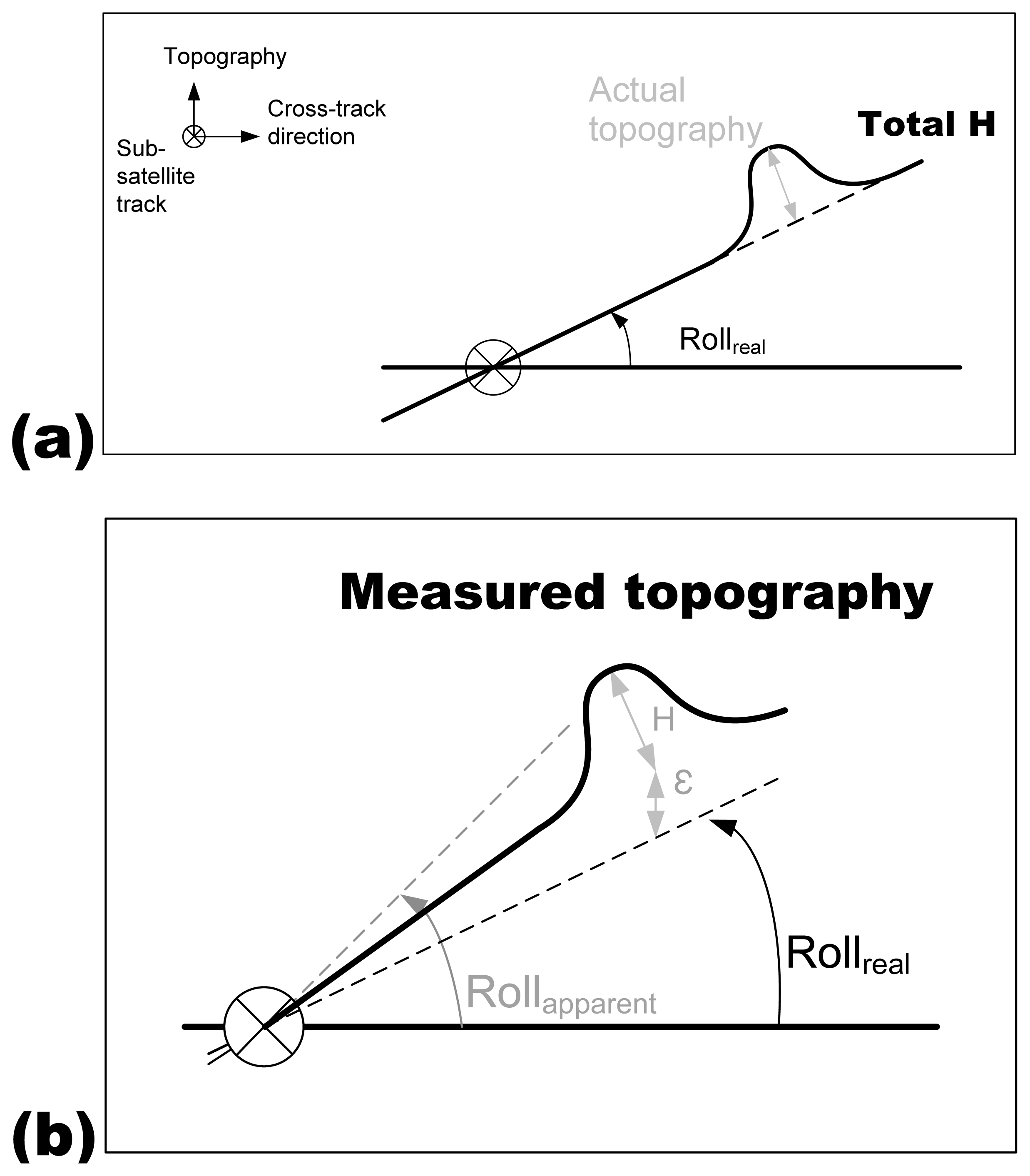
1.3. The Roll Paradigm
1.4. Empirical Cross-Calibration
- Their residual error was quantified as a total RMS, whereas the proposed SWOT mission’s error budget is now addressed as the sum of the power spectral density (PSD) laws for each error source: for which range of wavelengths can we expect ground calibration to be efficient and what is the limit?
- Would SWOT’s roll calibration require inputs from the constellation of nadir altimeters?
- What is the performance of the two new methods they describe but did not implement: 1/the collinear method and 2/the neighbor or sub-cycle method?
- Lastly, they discussed the importance of the orbit, but they did not address the rationale and possible benefits of using a “roll contingency” orbit that would more suitable for roll calibration.
1.5. Objective of This Paper
- To carry out performance assessments in the wavenumber domain, and to try and understand why some methods are more efficient for long/short wavelengths,
- To implement all four calibration methods and compare their relative performance as a function of the density and geometry of different calibration zones,
- To quantify the benefits of using the so-called “contingency orbit” and the nadir constellation to improve the empirical roll correction,
- To use more recent SWOT design items: orbits, white noise level, input roll before calibration.
2. Methodology
- along 1D profiles of nadir altimetry missions (Jason-CS and Sentinel-3 would be concurrent with SWOT) with a resolution of 7 km
- along 1D profile of SWOT’s nadir with a resolution of 7 km
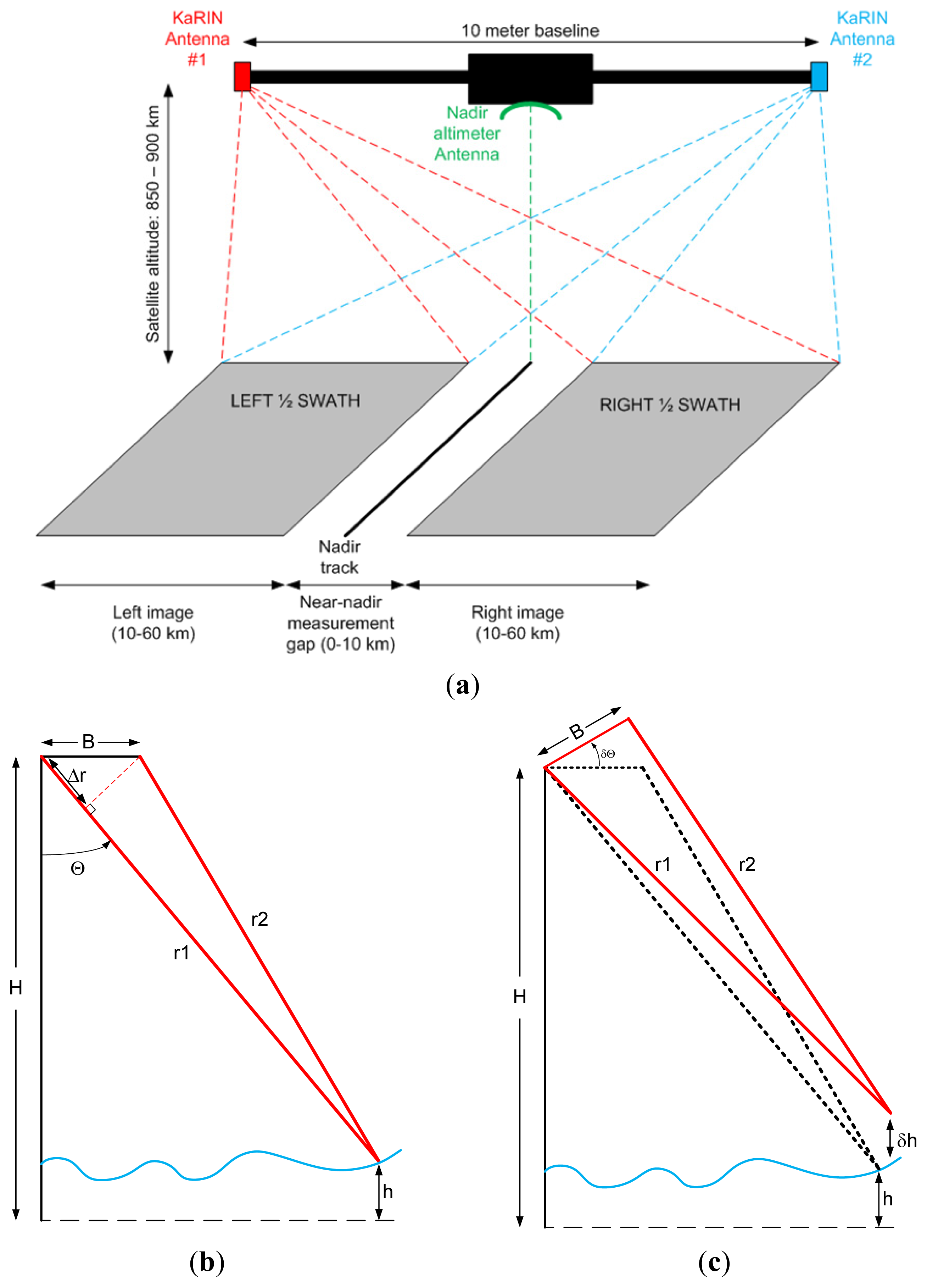
- in the 2D swath of KaRIN (geometry from Figure 1a) with resolution of 5 km.
2.1. Observations
2.2. Problem Solving
3. Spectral Separation of Roll from Other Cross-Track Gradients
3.1. Pitfalls of Empirical Roll Calibration
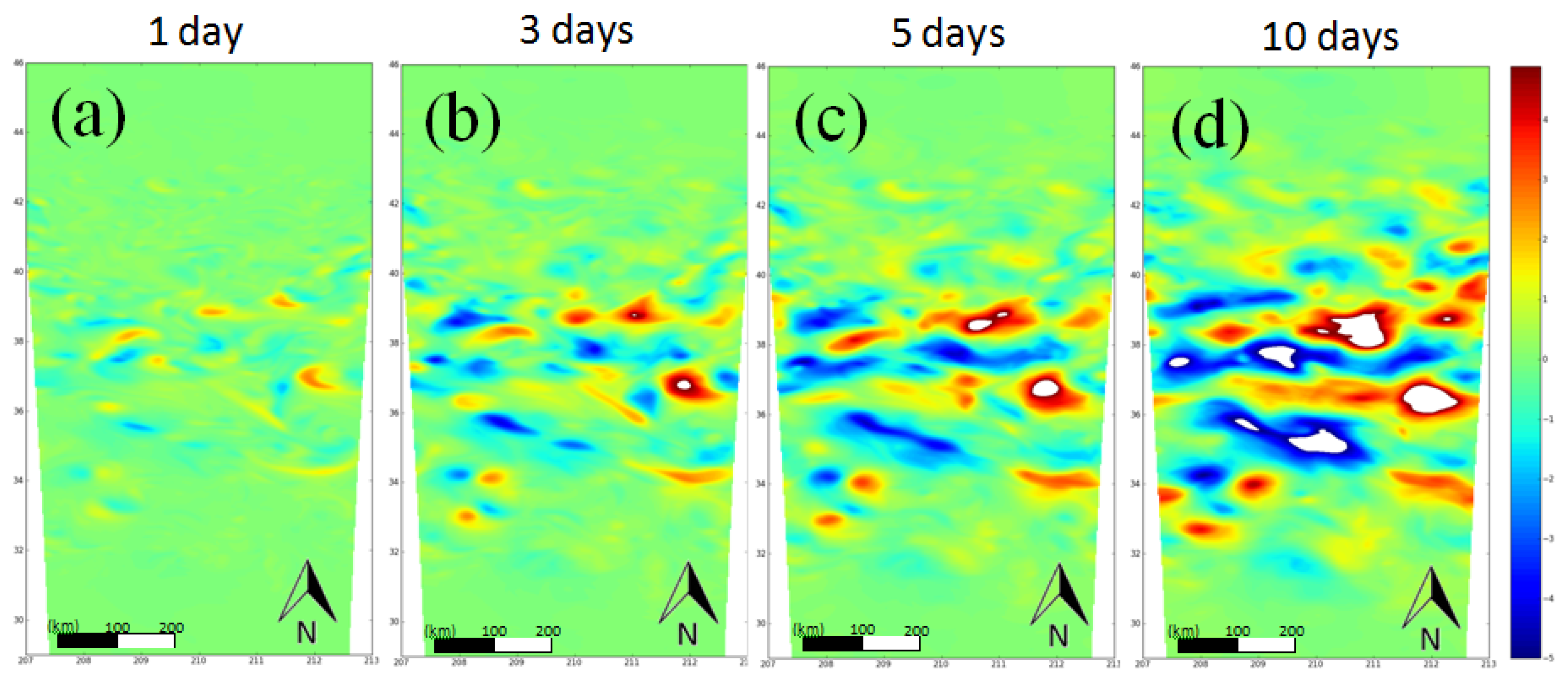
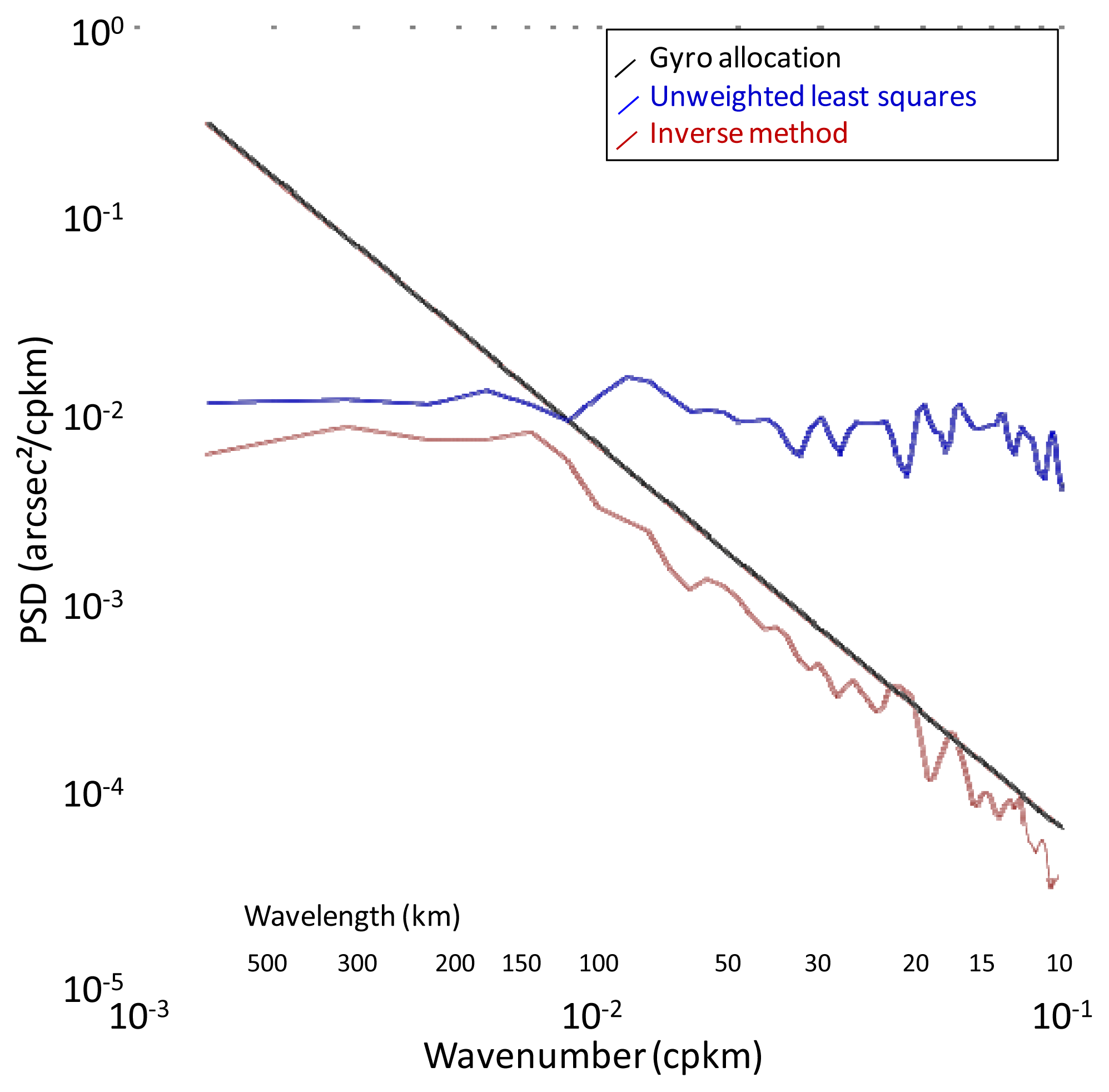
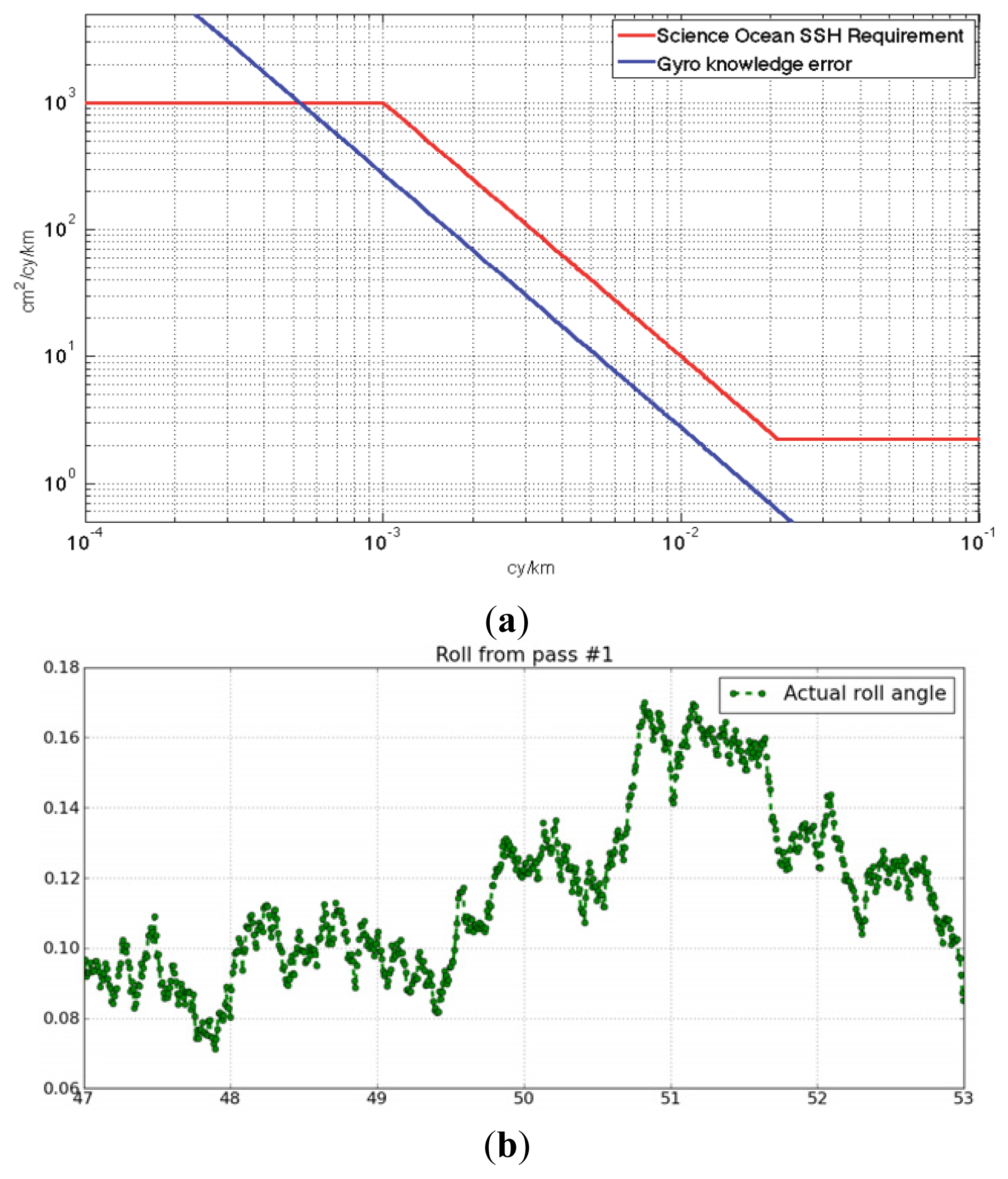
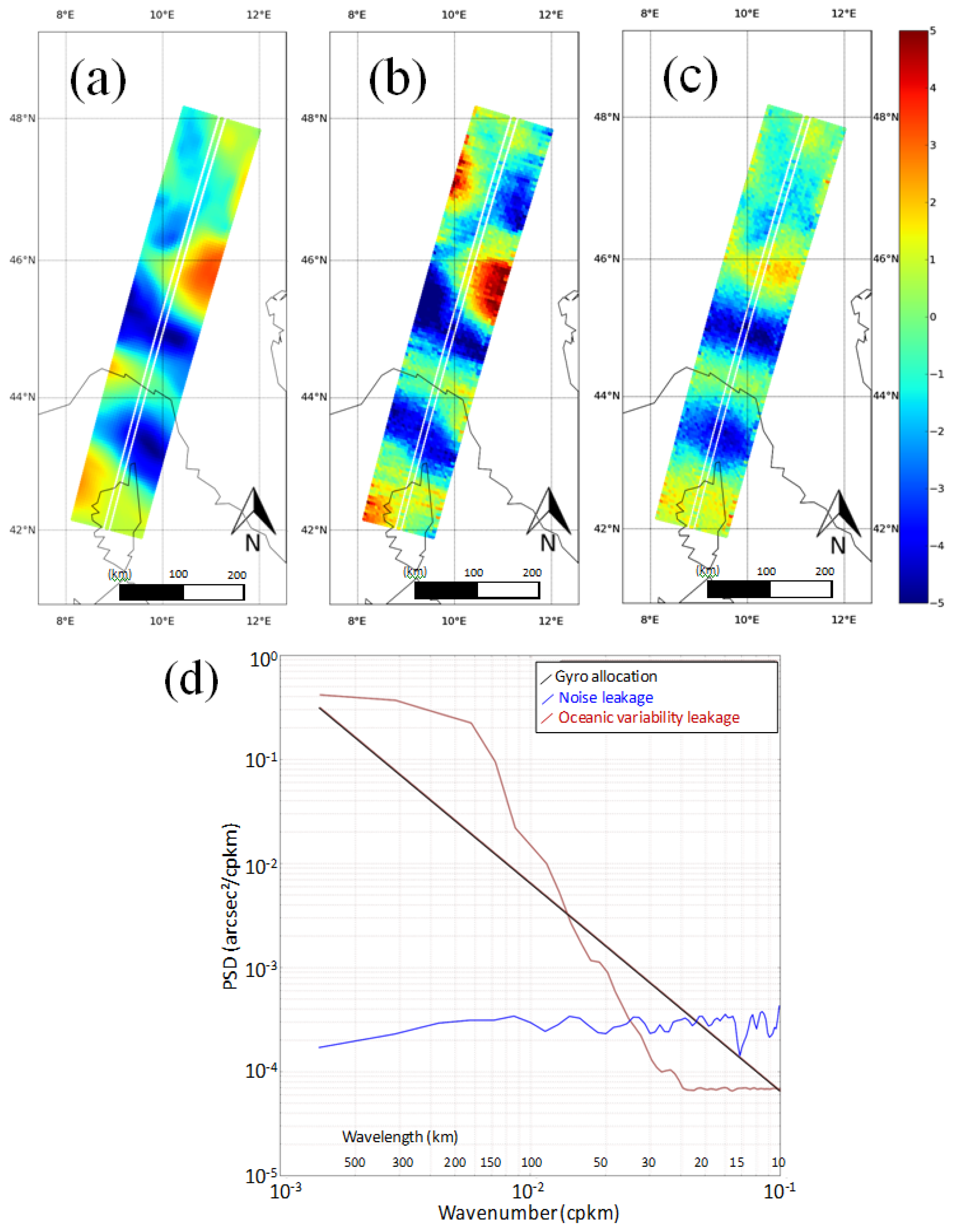
- In the first experiment (blue spectrum), we set the oceanic variability to zero in order to measure how instrumental noise (e.g., Figure 3d) would leak on our roll estimate if it was solved with Equation (5). As expected, the leakage artifact looks like Gaussian noise on our roll estimate, and it is primarily a problem for higher frequencies. This effect is amplified because the standard deviation of the instrumental noise is higher in the outer edges of the swaths, thus also increasing the probability to get a non-zero cross-track component that cannot be separated from actual roll.
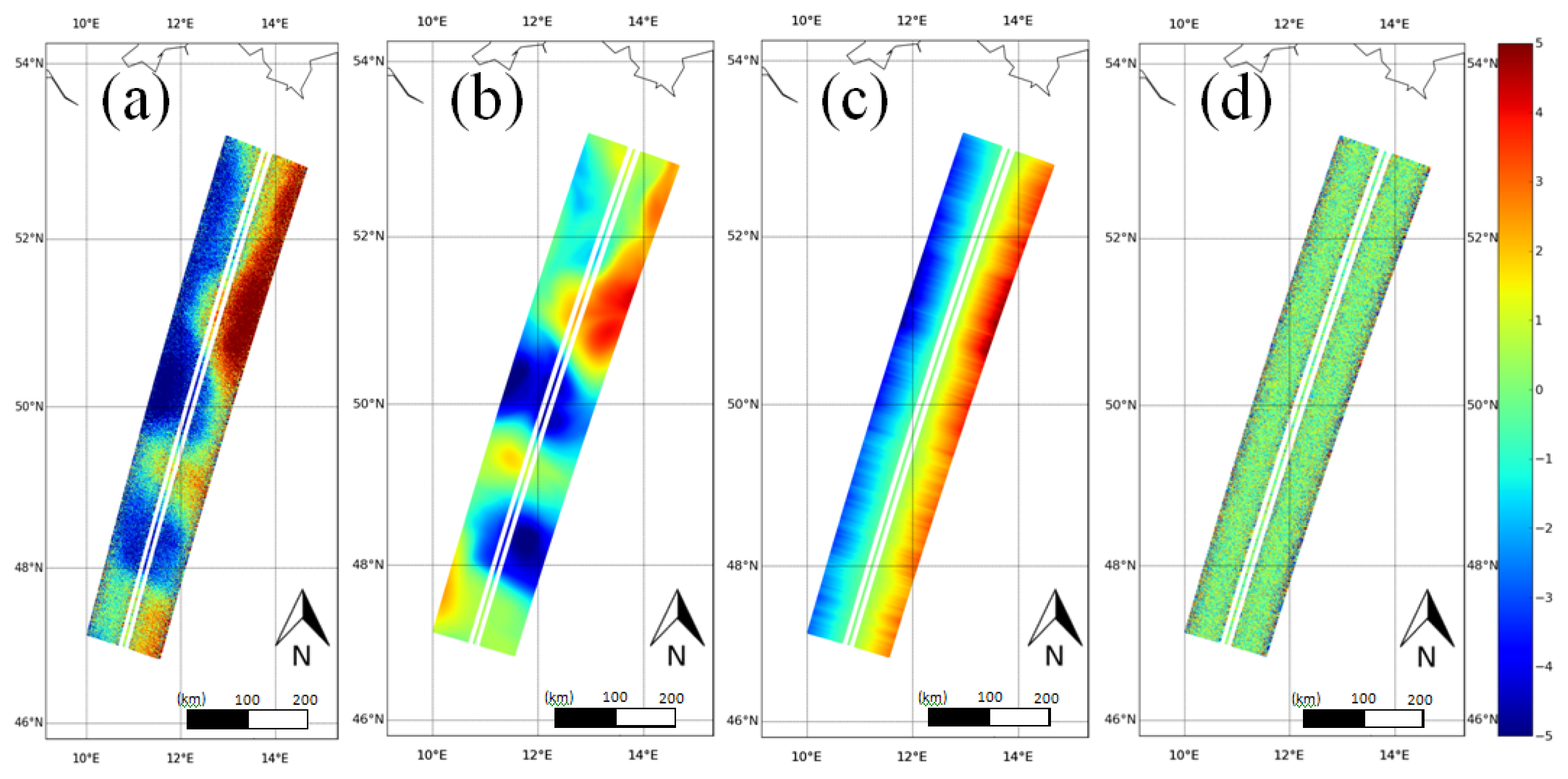
- In the second experiment (red spectrum), we set the instrumental noise to zero to measure how oceanic variability would leak on our roll estimate with Equation (5). The red spectrum indicates that the leakage primarily happens for wavelengths larger than 100 km. This is caused by the width of SWOT’s swath (120 km): large mesoscale structures (150–300 km) have a linear cross-track component hardly separable from actual roll because the instrumental field of view is not large enough.
- In the following sections, we try and understand how such leakage can be mitigated by using a nadir constellation proxy or image-to-image differences (problem described with Equations (2) to (4) instead of Equation (1)), and by using an inverse method that exploits our statistical knowledge of roll and oceanic signal spectra (problem solved with Equation (6) instead of Equation (5)).
3.2. Benefit and Limit of Using Image Differences
- Crossovers: when the swath from an ascending (respectively descending) arc crosses the swath of a descending (resp. ascending) arc.
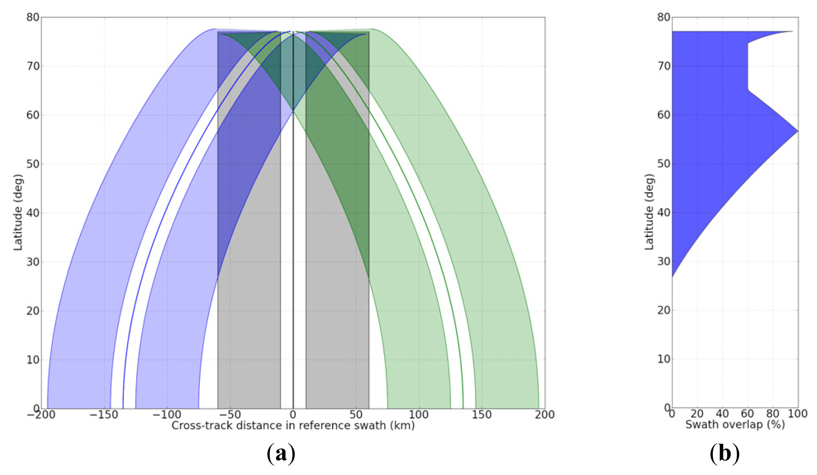
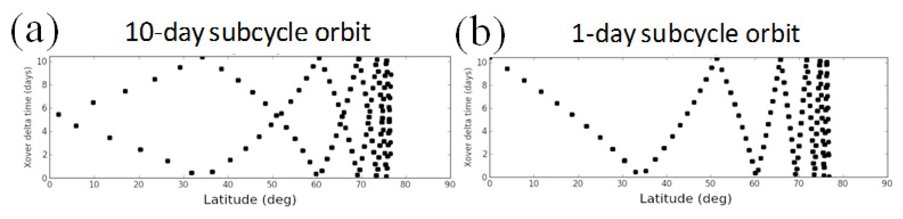
- Sub-cycle: when the proposed SWOT mission would be on its final orbit with a 21-day repeat cycle, adjoining swaths would start to overlap at low to mid latitudes.
- Collinear: SWOT’s revisit time and reference track would be controlled, so SWOT images would be almost perfectly co-located every repeat cycle (e.g., one-day cycle with the commissioning/CalVal orbit).
3.3. Further Mitigating Leakage on Roll
3.3.1. Nadir Constellation Proxy
3.3.2. Inverse Method
3.4. Summary: Observability Rules
- O1: The larger the calibration scene, the easier it is to achieve the spectral separation. Ideally, one would need a scene with a radius > 500 km (i.e., more than three times the radius from Chelton et al. [10] or Le Traon et al. [12]), but in practice the limit would be KaRIN’s field of view or less (e.g., sub-cycle and crossover overlaps could be smaller than 60 km).
- O2: One can enhance spectral separation with an image-to-image difference. The shorter the temporal distance between co-located pixels, the better the spectral separation is. Because a larger fraction of the variability is removed in the difference (smaller amplitude), and because rapid features are also smaller in size (the relative size of the calibration scene increases).
- O3: Spectral separation is enhanced by removing external content derived from the nadir constellation. The benefit to use nadir-derived maps is inversely proportional to the scene/method’s compliance to O1 and O2. In other words, if the scene is small or if a substantial fraction of mesoscale cannot be cancelled with an image-to-image difference, then external content from nadir maps would become a necessary input for roll calibration.
4. Understanding the Performance of the 4 Cross-Calibration Methods
4.1. Direct Method
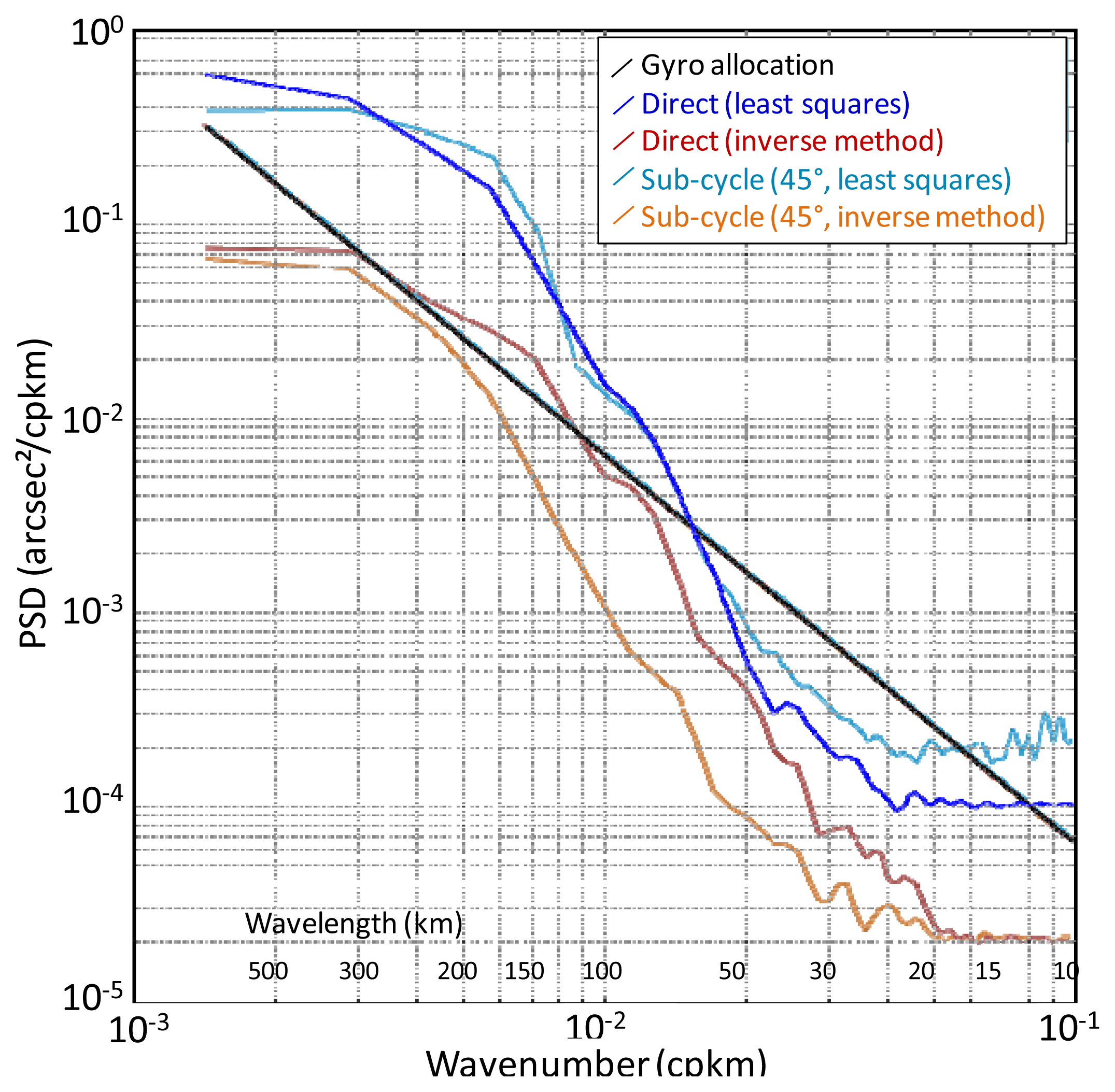
- The direct inversion is done using the full extent of the 120-km wide swath. This large cross-track field of view makes it easier to separate true roll from small mesoscale signatures (rule O1). This is emphasized between 20 and 60 km because the roundish shapes of mesoscale and cross-track roll gradients are visually and numerically easy to separate. For longer wavelengths, mesoscale structures are observed only partially in the geometry from Figure 1a (two 1/2 swaths of 50 km each) and roll and mesoscale are more difficult to separate.
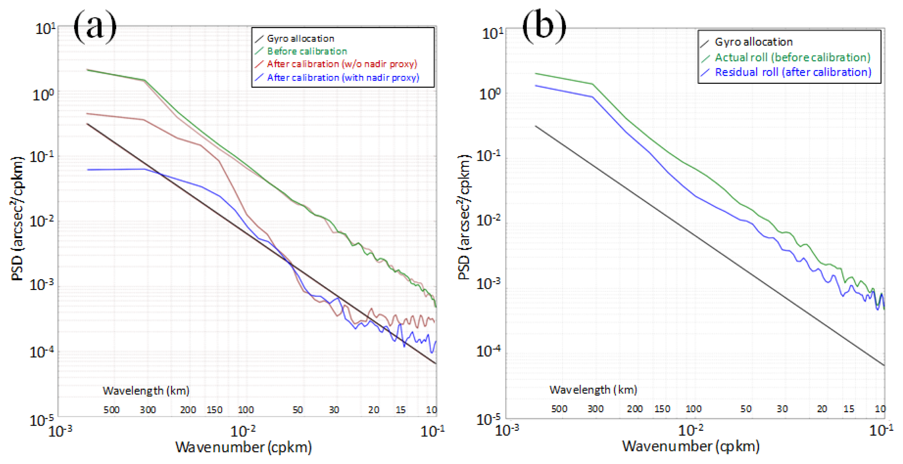
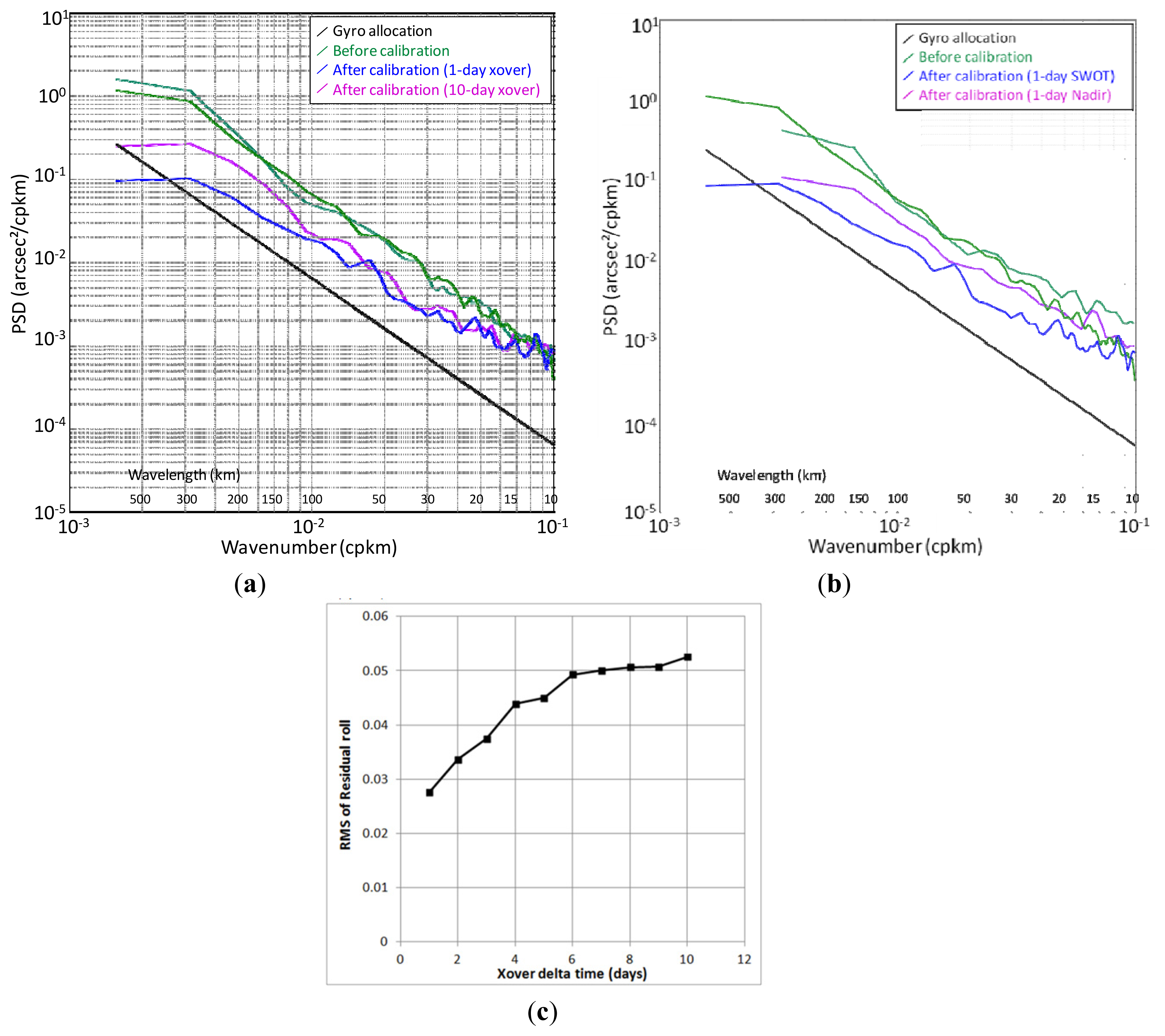
- For wavelengths longer than 150–200 km, the nadir constellation proxy accounts for the bulk of mesoscale gradients, which could be misinterpreted as roll (rule O3). This ability of the nadir constellation proxy to mitigate leakage is visible in the difference between the red (without proxy) and blue (with proxy) spectra from Figure 12a.
- Incidentally, because our covariance error model Cvv is focused on the smaller scales of mesoscale residuals after the proxy removal (Figure 9c), we also observe an improvement for high-frequency roll as well. When the proxy is not used, the model in Cvv is dominated by large mesoscale, which slightly increases the leakage of smaller structures and noise.
4.2. Collinear Method
4.3. Crossover Method
4.3.1. Calibration Zones
4.3.2. Performance
4.4. Subcycle Method
4.4.1. Calibration Zones
4.4.2. Performance
4.5. Summary
4.5.1. Baseline Orbit
4.5.2. Contingency Orbit
4.5.3. Commisioning/CalVal Orbit
5. Discussion and Outlook
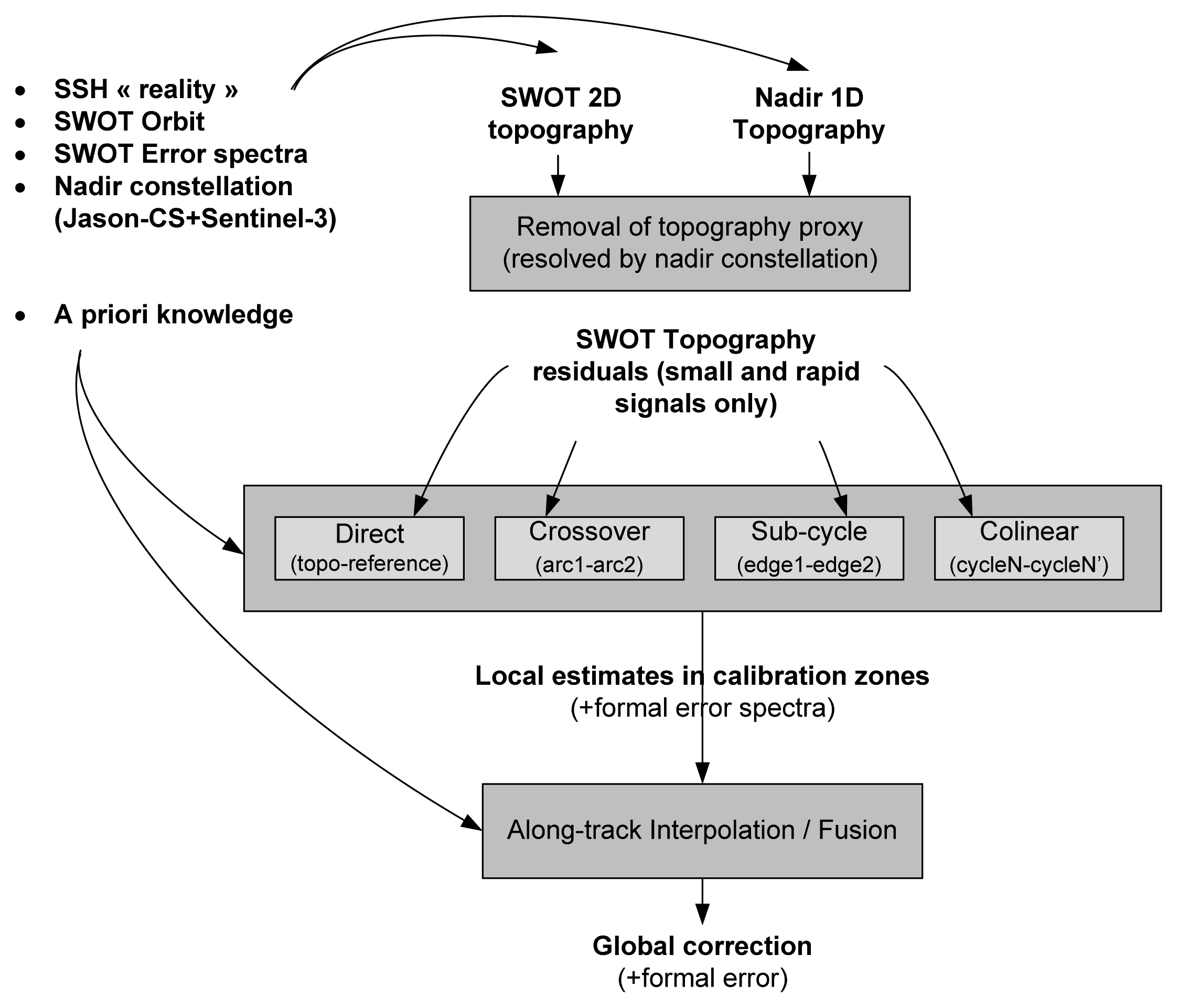
5.1. End-to-End Performance and the Fusion Mechanism
5.2. Methodology Improvements
5.3. Realistic Input Scenario
- What part of the oceanic variability should be preserved? Our SSH derived from Klein et al. [8] could be improved upon: larger or even global simulation area to account for regional variations in mesoscale and sub-mesoscale (e.g., Western boundary current VS “eddy desert”), or different physics (e.g., internal tides or waves).
- What is a realistic contingency scenario for uncalibrated roll (e.g., what are the residuals if a high-end gyroscope prediction is used)? Our “worst-case” scenario is quite pessimistic because in reality SWOT’s roll is unlikely to be that high for all frequencies. The benefit of using method X or Y and the benefit of the contingency orbit might be substantially changed by the wavelengths where the roll risk is the highest.
- What is the spectrum of the other SWOT errors with a cross-track signature that should be accounted for? Should we even try to separate them from roll? For instance: the wet troposphere path delay could result in a topography error with cross-track gradients (e.g., Ubelmann et al. [15]). Should roll-oriented simulations assume that the radiometer-based correction has small cross-track residuals and should roll calibration account for those in an empirical way?
- To what extent can a better Href proxy (Equation (2)) be available by SWOT’s launch? To illustrate, CNES has recently confirmed that SWOT would feature a Jason-class altimeter (no longer optional) and this sensor would provide an additional nadir measurement (at the same measurement time as KaRIN) able to improve the constellation proxy from Equation (2) (ours is based on Jason-CS and Sentinel-3). New interpolation methods and ocean models with assimilation could also provide a more efficient alternative to our simple AVISO-like map.
- How does the contingency algorithm need to account for land products and coastal transitions? In this paper, we focused on the ocean, following the rationale of [6] for SWOT’s baseline error budget. However this might need to be revisited in a contingency plan: if roll is higher than previously anticipated, inland hydrology measurements might require a more sophisticated algorithm sequence than the baseline outlined by Enjolras et al. [7]. Similarly, we ignored the case of coastal transitions, whereas the calibration scenes and the method performance is likely to be very different. This might require the development of land-specific roll calibration and a careful hydrology-oriented and coastal-oriented analysis of the interpolation/propagation mechanism discussed in Section 5.1.
6. Conclusions
Acknowledgments
Conflicts of Interest
- Author ContributionsGerald Dibarboure developed the roll calibration with four inverse methods, processed input model snapshots and nadir constellation snapshots, and carried out performance estimations in the spectral domain, and wrote the initial manuscript. Clement Ubelmann helped expanding the research focus, prototyped the sub-cycle method, carried out additional simulations and sensitivity tests with the sub-cycle method and contingency orbit, and assisted with manuscript writing.
References
- Dibarboure, G.; Labroue, S.; Ablain, M.; Fjortoft, R.; Mallet, A.; Lambin, J.; Souyris, J.-C. Empirical cross-calibration of coherent SWOT errors using external references and the altimetry constellation. IEEE Trans. Geosci. Remote Sens 2012, 50, 2325–2344. [Google Scholar]
- Durand, M.; Fu, L.-L.; Lettenmaier, D.; Alsdorf, D.; Rodriguez, E.; Esteban-Fernandez, D. The surface water and ocean topography mission: Observing terrestrial surface water and oceanic submesoscale eddies. Proc. IEEE 2010, 98, 766–779. [Google Scholar]
- Fu, L.L.; Rodriguez, E. High-Resolution Measurement of Ocean Surface Topography by Radar Interferometry for Oceanographic and Geophysical Applications. In The State of the Planet: Frontiers and Challenges in Geophysics; IUGG Geophysical Monograph; American Geophysical Union: Washington, DC, USA, 2004; Volume 19, pp. 209–224. [Google Scholar]
- Dibarboure, G.; Schaeffer, P.; Escudier, P.; Pujol, M.-I.; Legeais, J.F.; Faugère, Y.; Morrow, R.; Willis, J.K.; Lambin, J.; Berthias, J.-P.; et al. Finding desirable orbit options for the “extension of life” phase of jason-1. Mar. Geod 2012, 35, 363–399. [Google Scholar]
- Rosen, P.; Hensley, S.; Joughin, I.R.; Li, F.K.; Madsen, S.; Rodriguez, E.; Goldstin, R. Synthetic aperture radar interferometry. Proc. IEEE 2000, 88, 333–382. [Google Scholar]
- Esteban-Fernandez, D. SWOT Mission Performance and Error Budget; NASA/JPL Document (Reference: JPL D-79084); Jet Propulsion Laboratory: Pasadena, CA, USA, 2013. [Google Scholar]
- Enjolras, V.; Vincent, P.; Souyris, J.-C.; Rodriguez, E.; Phalippou, L.; Cazenave, A. Performances study of interferometric radar altimeters: From the instrument to the global mission definition. Sensors 2006, 6, 164–192. [Google Scholar]
- Klein, P.; Hua, B.L.; Lapeyre, G.; Capet, X.; le Gentil, S.; Sasaki, H. Upper ocean turbulence from high-resolution 3D simulations. J. Phys. Oceanogr 2008, 38, 1748–1763. [Google Scholar]
- Dibarboure, G.; Pujol, M.-I.; Briol, F.; le Traon, P.Y.; Larnicol, G.; Picot, N.; Mertz, F.; Ablain, M. Jason-2 in DUACS: First tandem results and impact on processing and products. Mar. Geod 2011, 34, 214–241. [Google Scholar]
- Chelton, D.B.; Schlax, M.G. The accuracies of smoothed sea surface height fields constructed from tandem altimeter datasets. J. Atmos. Ocean. Technol 2003, 20, 1276–1302. [Google Scholar]
- Bretherton, F.P.; Davis, R.E.; Fandry, C.B. A technique for objective analysis and design of oceanographic experiment applied to MODE-73. Deep-Sea Res 1976, 23, 559–582. [Google Scholar]
- Le Traon, P.Y.; Faugère, Y.; Hernandez, F.; Dorandeu, J.; Mertz, F.; Ablain, M. Can we merge GEOSAT follow-on with TOPEX/POSEIDON and ERS-2 for an improved description of the ocean circulation? J. Atmos. Ocean. Technol 2003, 20, 889–895. [Google Scholar]
- Chelton, D.B.; Schlax, M.G.; Samelson, R.M. Global observations of nonlinear mesoscale eddies. Prog. Oceanogr 2011, 91, 167–216. [Google Scholar]
- Escudier, R.; Bouffard, J.; Pascual, A.; Poulain, P.-M.; Pujol, M.-I. Improvement of coastal and mesoscale observation from space: Application to the Northwestern Mediterranean Sea. Geophys. Res. Lett 2013, 40, 2148–2153. [Google Scholar]
- Ubelmann, C.; Fu, L.; Brown, S.; Peral, E.; Esteban-Fernandez, D. The effect of atmospheric water vapor content on the performance of future wide-swath ocean altimetry measurement. J. Atmos. Ocean. Technol 2014, in press. [Google Scholar]


| Cross-Calibration Method | ||||||
|---|---|---|---|---|---|---|
| Direct | Crossover (KaRIN only) | Crossover (Nadir) | Sub-Cycle | Collinear | ||
| Description of calibration zones | How many concurrent zones | 1 | 2 (<50°) to 4 (>60°) | 4 (<50°) to 8 (>60°) | 2 (<60°) or 3 (>60°) | No benefit from cycle-to cycle difference on this orbit |
| Geometry | Entire swath | Diamond | 1D Segment | Ribbon | ||
| Temporal variability | n/a | 0 to 10.9 days | 0 to 10.9 days | 10.9 days | ||
| Along-track (max) | >10.000 km | 100 km (near 70°) 800 km (equator) | 0–300 kmrarely up to 600 km | >5.000 km | ||
| Across-track | Entire swath | up to 130 km (diamond center) | 1–8 km(nadir footprint) | 1 km (26°) to 60 km (high latitudes) | ||
| Order of magnitude of the roll reduction in contingency (PSD uncalibrated / PSD calibrated) | 1 < l < 30 km | 5 to 15 | 1 to 2 | 0 to 2 | 1 to 1.5 | n/a |
| 30 < l < 150 km | 15 to 7 | 2 to 5 (best)1.5 to 4 (worst) | 1.5 to 2 | 1.5 to 2 (best)1 to 1.5 (worst) | ||
| 150 < l < 500 km | 7 to 20 | 5 to 10 (best)2 to 5 (worst) | 1.5 to 2 | 2 to 20 (best)1 to 5 (worst) | ||
| Best VS worst zones | Geographical variability | n/a | Moderate (butterfly deltaT variations) | n/a | High | n/a |
| Best latitudes | n/a | 20°–45°, 55°–65°, >75° | n/a | 45°–65°, >75° | ||
| Worst latitudes | n/a | <20°, 45°–55°, 65°–75° | n/a | <40° | ||
| Void latitudes | n/a | n/a | n/a | <26° | ||
| Reliance on external nadirs | Very High for l < 100 km | Moderate | Very high | High (10-day subcycle) | n/a | |
| Cross-Calibration Method | ||||||
|---|---|---|---|---|---|---|
| Direct | Crossover (KaRIN only) | Crossover (Nadir) | Sub-Cycle | Collinear | ||
| Description of calibration zones | How many concurrent zones | 1 | 2 (<50°) to 4 (>60°) | 4 (<50°) to 8 (>60°) | 2 (<60°) or 3 (>60°) | No benefit from cycle-to cycle difference on this orbit |
| Geometry | Entire swath | Diamond | 1D Segment | Ribbon | ||
| Temporal variability | n/a | 0 to 10.9 days | 0 to 10.9 days | 1 day | ||
| Along-track (max) | >10.000 km | 100 km (near 70°)800 km (equator) | 0–300 kmrarely up to 600 km | >5.000 km | ||
| Across-track | Entire swath | up to 130 km (diamond center) | 1–8 km(nadir footprint) | 1 km (26°) to 60 km (high latitudes) | ||
| Order of magnitude of the roll reduction in contingency (PSD uncalibrated / PSD calibrated) | 1 < l < 30 km | 5 to 15 | 1 to 2 | 1 to 2 | 1 to 3 | n/a |
| 30 < l < 150 km | 15 to 7 | 2 to 5 (best)1.5 to 4 (worst) | 1.5 to 2 | 3 to 10 (best) 1 to 3 (worst) | ||
| 150 < l < 500 km | 7 to 20 | 5 to 10 (best)2 to 5 (worst) | 1.5 to 2 | 10 to 100 (best) 1 to 5 (worst) | ||
| Best VS worst zones | Geographical variability | n/a | Very high (V-shaped deltaT variations) | n/a | High | n/a |
| Best latitudes | n/a | 20°–45°, 55°–65°, >75° | n/a | 45°–65°, >75° | ||
| Worst latitudes | n/a | <20°, 45°–55°, 65°–75° | n/a | <40° | ||
| Void latitudes | n/a | n/a | n/a | <26° | ||
| Reliance on external nadirs | Very High for l < 100 km | High (xover with deltaT < 5d latitude gaps) | Very high | Very low(1-day sub-cycle) | n/a | |
| Cross-Calibration Method | ||||||
|---|---|---|---|---|---|---|
| Direct | Crossover (KaRIN only) | Crossover (Nadir) | Sub-Cycle | Collinear | ||
| Description of calibration zones | How many concurrent zones | 1 | 1 (very sparse coverage | 4 (<50°) to 8 (>60°) | Non-existent on this orbit | Entire swath |
| Geometry | Entire swath | Diamond | 1D Segment | Entire swath | ||
| Temporal variability | n/a | 0 to 1 day | 0 to 1 day | 1-day | ||
| Along-track (max) | >10.000 km | 100 km (near 70°)800 km (equator) | 0–300 kmrarely up to 600 km | >10.000 km | ||
| Across-track | Entire swath | up to 130 km (diamond center) | 1–8 km(nadir footprint) | Entire swath | ||
| Order of magnitude of the roll reduction in contingency (PSD uncalibrated / PSD calibrated) | 1 < l < 30 km | 5 to 15 | 1 to 2 | 1 to 2 | n/a | <1.5 |
| 30 < l < 150 km | 15 to 7 | 2 to 5 | 1.5 to 2 | 1.5 to 2 | ||
| 150 < l < 500 km | 7 to 20 | 5 to 10 | 1.5 to 2 | 1.5 to 2 | ||
| Best VS worst zones | Geographical variability | n/a | Very sparse coverage (<20%) | n/a | n/a | n/a |
| Best latitudes | n/a | n/a | n/a | n/a | ||
| Worst latitudes | n/a | n/a | n/a | n/a | ||
| Void latitudes | n/a | Very large (>80%) | n/a | n/a | ||
| Reliance on external nadirs | Very High for l < 100 km | Very low (always short deltaT) | Very high | n/a | None | |
© 2014 by the authors; licensee MDPI, Basel, Switzerland This article is an open access article distributed under the terms and conditions of the Creative Commons Attribution license (http://creativecommons.org/licenses/by/3.0/).
Share and Cite
Dibarboure, G.; Ubelmann, C. Investigating the Performance of Four Empirical Cross-Calibration Methods for the Proposed SWOT Mission. Remote Sens. 2014, 6, 4831-4869. https://doi.org/10.3390/rs6064831
Dibarboure G, Ubelmann C. Investigating the Performance of Four Empirical Cross-Calibration Methods for the Proposed SWOT Mission. Remote Sensing. 2014; 6(6):4831-4869. https://doi.org/10.3390/rs6064831
Chicago/Turabian StyleDibarboure, Gerald, and Clement Ubelmann. 2014. "Investigating the Performance of Four Empirical Cross-Calibration Methods for the Proposed SWOT Mission" Remote Sensing 6, no. 6: 4831-4869. https://doi.org/10.3390/rs6064831
APA StyleDibarboure, G., & Ubelmann, C. (2014). Investigating the Performance of Four Empirical Cross-Calibration Methods for the Proposed SWOT Mission. Remote Sensing, 6(6), 4831-4869. https://doi.org/10.3390/rs6064831