Calibrated Full-Waveform Airborne Laser Scanning for 3D Object Segmentation


Abstract
: Segmentation of urban features is considered a major research challenge in the fields of photogrammetry and remote sensing. However, the dense datasets now readily available through airborne laser scanning (ALS) offer increased potential for 3D object segmentation. Such potential is further augmented by the availability of full-waveform (FWF) ALS data. FWF ALS has demonstrated enhanced performance in segmentation and classification through the additional physical observables which can be provided alongside standard geometric information. However, use of FWF information is not recommended without prior radiometric calibration, taking into account all parameters affecting the backscatter energy. This paper reports the implementation of a radiometric calibration workflow for FWF ALS data, and demonstrates how the resultant FWF information can be used to improve segmentation of an urban area. The developed segmentation algorithm presents a novel approach which uses the calibrated backscatter cross-section as a weighting function to estimate the segmentation similarity measure. The normal vector and the local Euclidian distance are used as criteria to segment the point clouds through a region growing approach. The paper demonstrates the potential to enhance 3D object segmentation in urban areas by integrating the FWF physical backscattered energy alongside geometric information. The method is demonstrated through application to an interest area sampled from a relatively dense FWF ALS dataset. The results are assessed through comparison to those delivered from utilising only geometric information. Validation against a manual segmentation demonstrates a successful automatic implementation, achieving a segmentation accuracy of 82%, and out-performs a purely geometric approach.1. Introduction
Airborne laser scanning (ALS) is a remote measurement technique that has seen rapid uptake in the photogrammetric community for determination of the geometry of the Earth’s surface in a rapid and accurate manner [1]. ALS has become an increasingly important technique for delivering a quantitative 3D digital representation of surface features for a range of enduser applications [2]. Not only can ALS deliver geometric information relating to Earth surface features, it can also provide additional information about the backscattering properties of the illuminated surface in physical form. In the case of conventional discrete-return ALS, the recorded physical information relates to the intensity response, while more recently it has become possible through full-waveform (FWF) ALS to record the complete backscattered signal. Whereas discrete-return ALS is only capable of registering a limited number (usually up to five) returns from a single transmitted pulse, FWF ALS digitises the complete profile of the received energy, and stores this as a waveform, encapsulating the interaction of the transmitted pulse with surface targets. This allows the interpretation of additional physical backscattering information such as roughness and reflectivity for the illuminated target [3]. To fully exploit this additional FWF information, end user applications require automated processing of this massive information for tasks such as 3D object recognition and feature extraction [4].
2. Background
2.1. 3D Object Segmentation
The aim of 3D object segmentation is to group points of similar attributes in 3D space into meaningful regions/segments to represent features of interest [5]. Segments should be spatially connected and related to objects with similar attributes, such as planes, cylinders, or sphere surfaces [6]. Many 3D point cloud segmentation approaches have been presented in the literature for various applications. These methods can be differentiated in terms of segmentation algorithm and criteria used to define the similarity between the given points, or the routine implemented to grow seed points into regions [2]. Many segmentation approaches are based on the Hough transform and the RANdom SAmple Consensus (RANSAC) methods to deliver similarity measures, while surface growing and scanline segmentation are popular routines used in computer vision applications to segment regions automatically [2]. All these approaches are either purely geometrybased, or augment geometric information with radiometric measurements to improve segmentation results. However, performance is relative to the complexity of the data and the selected interest area. This is mainly because of shortcomings in the calibration process of the integrated additional information, and also in the exploitation scenario of the additional information to deliver the similarity measure of the segmentation technique.
In order to efficiently identify surface features from unstructured 3D point clouds, sets of points should be modelled into functional structured shapes. These shapes can be delivered from segmentation processes by adopting a suitable similarity measure to group points into distinct clusters. In theory, and in the case of dense datasets, planes can efficiently define most types of complex object, with even spheres and cylinders capable of being represented by the normal vector. The normal vector is a particularly popular segmentation criterion for 3D point cloud data, as it can deliver reliable results even in the presence of noise [7]. However, this is only true when the neighbourhood definition is selected properly. Normal vector segmentation techniques can detect sharp edges, as well as flat or highly curved surfaces [8]. Some authors have incorporated additional attributes to emphasise certain behaviours and avoid mis-clustering results, the majority of these methods being designed to improve discrimination between surfaces of similar characteristics.
The integration of ALS geometry and intensity values to improve 3D segmentation of glacier surfaces has been evaluated by [9], who demonstrate that joint exploitation is more effective than using an individual information source alone. It was also shown by [10] that accurate modelling of a water surface can be delivered from ALS data when combining intensity with standard geometric information. However, the additional observables from FWF can provide further useful information for segmentation and classification [11]. The backscatter energy from FWF offers significant potential to better identify surface features by delivering information on surface roughness and reflectivity [12]. Integrating this information alongside standard geometric information can therefore enhance results in comparison to relying on geometric information alone [13].
The majority of existing studies which utilise FWF ALS for segmentation have been developed to characterise trees for forestry applications [5,14]. One such pioneering study was the approach presented by [15] who considered the eigenvalues from the covariance matrix. Consequently,[15] claimed that FWF analysis yields improved information content, leading to better object identification and resulting in more precise segmentation results (potential that was also demonstrated by [16]). In a different approach,[14] relied on the echo width from FWF ALS to define the roughness criterion in asurface growing algorithm to segment vegetation. This delivered significant improvements in separating tall vegetation from non-vegetation echoes in urban areas. The normalised cut segmentation approach, initially presented by [17] for image segmentation, was adopted to define single trees and tackle drawbacks in stem detection approaches. FWF echo amplitude and width parameters were exploited alongside the coordinates of the detected voxels to identify trees, significantly improving tree detection results. Furthermore, exploiting FWF information (FWF stacking) to segment man-made surfaces in urban areas was investigated by [18], demonstrating further potential to improve segmentation results.FWF additional information has also been integrated alongside geometric information to improve classification results in urban areas. This was demonstrated by [19] by making use of the backscatter coefficient as an attribute to discriminate classes through a decision tree approach. The study demonstrated the advantages of FWF ALS data over discrete return data to improve classification methodologies.
However, all previously available methods have weaknesses in discarding the presence of noise and fail to account for variations in data density which translates to shortcomings in defining minor and complex features. Many of these approaches also implement solutions which are dependent on a large number of parameters. Furthermore, a commonality of all available approaches could be described as a failure to distinguish between different features of similar geometric attributes, such as asphalt and paved ground or bare ground and mown grass. Therefore, an effective and reliable segmentation strategy is needed to overcome such shortcomings.
2.2. Radiometric Calibration
Although integrating physical information from FWF ALS has been proven capable of improving segmentation results (as demonstrated through aforementioned examples), direct use of such information without prior radiometric calibration is not recommended [20,21]. This is because the backscatter signal, which is a modified form of the transmitted pulse [22], is affected by many variables during travel between the sensor and the Earth’s surface. This includes sensor properties, flying height and target characteristics [23]. It is therefore generally acknowledged that rigorous radiometric calibration should be undertaken prior to full exploitation of FWF ALS data in order to normalise these effects [24].
Numerous studies have concentrated on calibrating intensity values delivered from discrete-return ALS systems to improve the quality of the final products. However, while intensity is only able to represent the reflectance of the echo target, the additional physical information derived from FWF encapsulates all target characteristics (i.e., reflectance, area, orientation). Two methods are presented by [9] for intensity correction: data-driven and model-driven. Both methods were found to successfully correct intensity values and were well-suited for implementation on large datasets. However, the model-driven approach was found to be preferable as measurements were not required from multiple flying heights [9].A combined geometric and radiometric calibration routine for ALS data is presented by [25] to improve land-cover classification. A physical model based on the radar equation was applied to calibrate intensity by taking sensor properties, topographic effects and atmospheric attenuation into consideration. After implementation, improvements in the classification results of up to 11.6% were observed [25].It has been claimed by [26] that when using portable artificial reference targets in the radiometric calibration routine, the calibrated intensity data would facilitate improved classification and segmentation of vegetation and other land-cover types. A similar approach was later presented by[27],thoughin this case using natural reference targets for the calibration process demonstrated better results. However, despite this progress towards more effective calibration of ALS radiometric information, intensity data are not representative of all parameters which affect the received backscattered energy. In this sense, physical observables from FWF systems provide a superior and more complete contribution.
As defined through the radar equation, the ALS backscatter cross-section (σ) is a measure of directional scattering power that encapsulates all target characteristics including scattering direction, reflectivity and area of illumination [28]. In FWF ALS systems and when using Gaussian decomposition to retrieve the echo waveform, such as in the case of the Rigorous Gaussian Detection (RGD) method [29], the received power can be represented as the product of echo amplitude and width [30]. Assuming that all unknowns in the radar equation are combined in one single constant, the calibration constant (Ccal) can be determined for a particular ALS campaign [31]. Once Ccal is determined, σ can be estimated for individual echoes across the entire dataset [20]. However, the backscatter coefficient (γ) offers benefits over the cross-section (σ), as the latter tends to be sensitive to different system and target characteristics [32]. When the incidence angle of the laser beam is altered, then the illumination area is also modified and therefore γ can be introduced as the backscatter cross-section normalised with respect to the illumination area [33]:
However, neither σ nor γ are free from the incidence angle effect [11]. Therefore both parameters can be normalised with respect to the incidence angle following the Lambertian scattering assumption as defined in Equations (2) and (3), respectively, and as proposed by [33].
This leads to four backscatter parameters: σ, γ, σα, and γα. Although these parameters are closely related, each development has shown capacity for generating enhanced results.
The potential of these parameters has been discussed by [34] for calibration of the FWF backscatter signal. Subsequent investigations by [31] developed this into a practical absolute radiometric calibration workflow. This approach utilised a natural reference target of known backscatter characteristics to derive the calibration constant for the entire flight campaign. In contrast with previously proposed approaches,[31] recommended that the reflectivity of the reference target should be measured in the field, at the time of the survey, using a portable reflectometer to ensure that atmospheric conditions are consistent with those which existed during data acquisition. Building on these findings,[32] distinguished between broad canopy and terrain (non-vegetation) echoes by applying the backscatter cross-section, σ. Following this, the 3D point cloud was classified into vegetation and non-vegetation classes with better than 90% accuracy [32]. A further improvement in classification performance was then demonstrated by [19], using σ in comparison to original echo amplitude signals.The improved performance of the γ parameterover σ for classification of 3D point clouds in FWF systems was subsequently demonstrated [30].
None of the aforementioned studies account for the effect of local incidence angle in the calibration process, the influence of which is demonstrated through the work of [27] in the context of intensity correction. Aiming to overcome this,[33] incorporated the incidence angle effect in the radiometric calibration workflow of [31]. Consequently, and by building upon the contribution of [19], [33] used the derived incidence angle to deliver the σα, and γα parameters for individual echoes. However, although the presented routine was found to be highly valid over planar features, results were uncertain over more challenging rough surfaces and terrain.
This paper focuses on the implementation of a radiometric calibration workflow for FWF ALS data, and demonstrates how the resultant FWF information can be used to improve segmentation of an urban area. The novelty of the presented approach is in the use of the calibrated backscatter parameters as a weighting function to estimate the segmentation similarity measure. The paper demonstrates the potential to enhance 3D object segmentation in urban areas by integrating the FWF physical backscattered energy alongside geometric information. The segmentation methodology is presented in detail to include similarity measure derivation and point grouping strategy. Results are assessed through comparison to outputs delivered from utilising only geometric information. Validation against a manual segmentation is also presented.
3. Study Area and Dataset
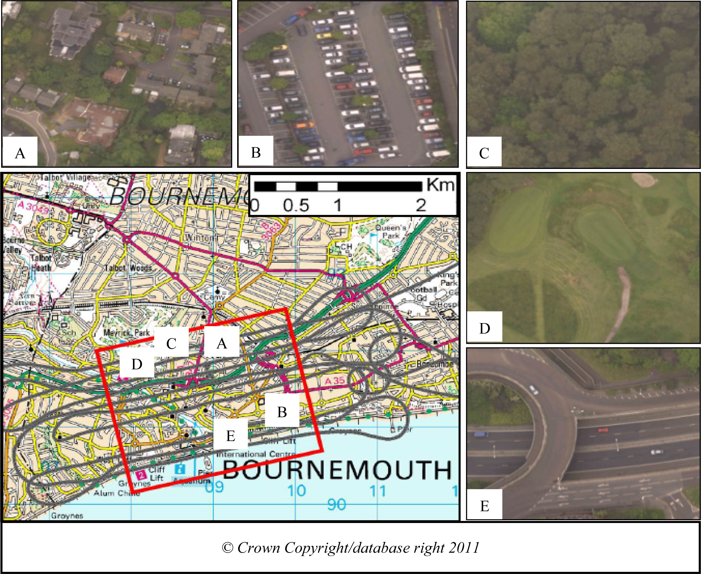
This study utilised small-footprint FWF ALS data acquired from a Riegl LMS-Q560 scanner, with a wavelength of 1550 nm. The technical specifications of this system are described in [35]. The test data covers part of the city of Bournemouth, located on the south coast of the UK, and is composed of both man-made and natural land-cover features (Figure 1). The dataset, which was collected from a helicopter platform in May 2008, has an average flying height of 350m. This offers a relatively high point density of approximately 15 points/m2, with a 0.18 m diameter footprint. The ALS campaign was flown in leaf-on conditions with simultaneous colour imagery captured through a Hasselblad digital camera, and subsequently orthorectified with a ground sample distance (GSD) of 0.05 m. The ALS dataset, together with the trajectory information and orthophoto coverage, were provided by Ordnance Survey, Great Britain’s national mapping agency. The raw data were converted from waveforms to point data using the RGD post-processing method, as described by [21], and were transformed from WGS-84 to OSGB36 coordinates (UK National Grid).
4. Methodology
4.1. Radiometric Calibration
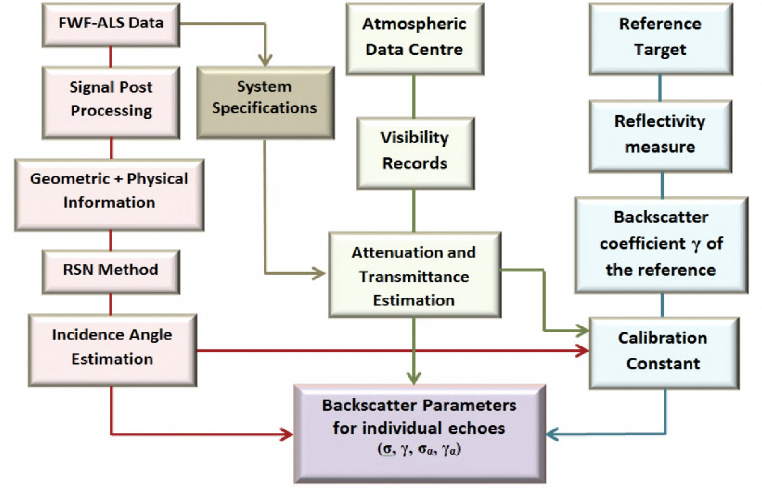
A practical and robust radiometric calibration routine, accounting for all variables affecting the backscattered energy, including the essential angle of incidence effect, is presented. The routine is based on the radar equation and relies on robust incidence angle estimation. Figure 2 illustrates the radiometric calibration workflow.
Following this, geometric and physical backscattering information is delivered for individual FWF echoes (e.g., 3D point location, echo width, echo amplitude, etc.). In order to calibrate the dataset, the four backscatter parameters (σ, γ, σα, γα) are determined for individual laser echoes. This is achieved by firstly estimating the incidence angle for individual echoes. Incidence angle is a function of illumination direction from the sensor to the target and the surface normal vector associated with the point. A novel approach for reliable estimation of local incidence angle, termed the robust surface normal (RSN) method, as described in [36], has been implemented here.
In order to undertake radiometric calibration, the RSN method was firstly applied to reference target echoes to account for the incidence angle effect on the reference target backscattered energy. It should be noted that artificial targets with known reflectivity were used to act as a reference for the calibration process. The energy loss due to atmospheric scattering and absorption during time of flight was considered in the calibration model. The atmospheric transmittance was estimated based on the model described by [9] and presented in Equation (4):
The atmospheric attenuation coefficient of the laser power is strongly affected by laser wavelength and visibility, with the latter obtained from the nearest meteorological station. Attenuation modelling was undertaken using the approach described by [37]:
As the backscatter coefficient (γ) has a close relationship with biconical reflectance [22], it was considered as the parameter of choice to estimate the calibration constant in this research [30]. An ideal Lambertian scatterer has been assumed in the case of the reference targets, with the incidence angle effect considered in the reflectivity computations. Calibration constants were then delivered for all reference target echoes based on the backscatter coefficient values[20,31]. Thus, all variables (including incidence angle and atmospheric effects) affecting the backscattered signal in travel between the sensor and the target were considered for reference targets echoes. To avoid the influence of noise, a mean calibration constant was then determined from all reference target echoes. This calibration constant was subsequently utilised for the determination of the four backscatter parameters (σ, γ, σα, γα) for individual echoes across the dataset.
The proposed radiometric calibration aimed to calibrate FWF backscatter signals by minimising the discrepancies between signals delivered from overlapping flightlines. To achieve this goal, it was proposed to identify the backscatter parameter that delivered the best agreement between signals from overlapping flightlines post-calibration; see [20] for details. Consequently, the four backscatter parameters (σ, γ, σα, γα) were investigated for individual echoes within selected regions in the test dataset. σα and γα parameters reveal the influence of the incidence angle effect on the reflected backscatter signal, and also reflect the performance of the RSN method.
4.2. Segmentation Routine
A segmentation methodology was developed with the aim of integrating the calibrated backscatter signals in order to overcome weaknesses in currently available approaches. The approach is fundamentally based on defining planimetric primitives, as these are the most basic geometric shapes in urban areas. The segmentation approach presented in this research adopted the following considerations:
The raw unstructured 3D point clouds were used as input. This included all echoes delivered from FWF post-processing;
Calibrated backscatter parameters were integrated with the geometric information;
As the normal vector was considered as the optimal criterion to define similarity between laser echoes [6] it was adopted as the main segmentation criterion;
The calibrated backscatter parameters were used as a weighting function in the normal vector definition to improve detection of points which exhibited similar characteristics (e.g., planarity, smoothness);
The method used pulse width and the number of return echoes to discriminate vegetation;
Due to well-documented reliability and flexibility (e.g.,[6]), a surface growing strategy was utilised to segment the point clouds.
Radiometric calibration analysis showed that no general assumption could be applied to all surface feature types when considering the optimal backscatter parameter to adopt in the segmentation routine. However, two main classes seem to be clearly distinguishable based on their surface roughness. These were vegetation and non-vegetation; however, it was not possible to differentiate between the two on the basis of an exact roughness value. Pulse width has previously been demonstrated to be the optimal parameter in terms of defining roughness [3,38,39]. Consequently, analysis was performed in order to assess the behaviour of pulse width over different land-cover types in the Bournemouth datasets. The goal of these analyses was to discriminate between land-cover classes in order to facilitate the selection of the optimal backscatter parameter to use in the segmentation routine. The segmentation routine included two main stages: segmentation criteria derivation, and segmentation strategy to group points into meaningful segments.
4.2.1. Segmentation Criteria Derivation
The normal vector is a well-established geometric criterion which can be used to define the orientation of 3D objects, and works efficiently in unstructured 3D point clouds [8]. It can define the measure of similarity between 3D points by identifying points that belong to the same surface, based on smoothness constraints [40]. However, the task of discriminating points with similar geometric characteristics but otherwise different physical attributes, such as artificial and natural bare ground, is an altogether greater challenge, and one which cannot be reliably addressed through geometric information alone. The backscatter parameters provided by FWF ALS are capable of defining the physical properties of the surface features. Therefore, an approach was developed to estimate the normal vector by integrating the backscatter parameters with standard geometric information and this formed the basis for segmentation of FWF echoes.
The normal for individual points was estimated using the robust surface normal (RSN) method developed by [36]. However, in this case, the weighting function in the moment invariant definition (used for individual echoes) was based on the calibrated backscatter parameters. As four different backscatter parameters (σ, γ, σα, γα) can be produced for individual echoes following the calibration workflow, a condition was set based on the surface roughness analysis to select the optimal backscatter parameter for individual echoes. The estimated normal vectors from the RSN method delivered residuals (φ) for individual points as an indicator of the uncertainty in the normal vector estimation due to noise effects (refer to [36]). These residuals were subsequently used in the surface growing algorithm to select seed points.
No general assumption can be applied to all surface feature types regarding the optimal backscatter parameter to use in segmentation. As outlined above, pulse width has been shown to be a reliable parameter to discriminate on the basis of surface roughness, and group points into rough and smooth surfaces. Simulation results presented by [3] for the same datasets as investigated here showed that a pulse width at half maximum value of 2.69 ns could be used to effectively group points into these two classes. However in reality, and especially over natural land cover, it is likely that there will be rough surfaces which do not necessarily represent vegetation. This aspect therefore has to be investigated in further detail to allow discrimination from vegetation based on FWF parameters.
To better understand the relationship between pulse width and roughness, pulse width was investigated and analysed over nine land-cover categories (Table 1). The examined categories included multiple targets from different land-cover types with varying levels of roughness. These targets were identified with the aid of orthophotography, and were derived from multiple flightlines and different regions of the study site. The mean of the pulse width values highlighted in bold in Table 1 represent categories with a mean pulse width >2.69 ns. Values in red represent rough surfaces which are not vegetation. Therefore another condition was required to discriminate non-vegetation from the rough class. The number of returns delivered from vegetation was observed as being greater than those delivered from non-vegetation. Therefore, a condition was proposed to use the number of returns in order to separate vegetation from non-vegetation echoes in the rough class.
If the pulse width is greater than 2.69ns then the target is classified under the rough class, otherwise it is assigned to the smooth class with the assignment of γα as the optimal backscatter parameter for use in segmentation. The rough class is then further evaluated, and when the number of returns is less than two, the target is assigned to the “rough non-vegetation” class, with γα applied as the optimal backscatter parameter. Targets in the rough class with greater than two returns are considered to bevegetation and the σ parameter is adopted. It should be noted that the smooth class not only includes perfectly smooth man-made features, but also regular surfaces such as hedges and mown grass, which exhibit a well-defined geometry in terms of incidence angle.
From a physical point of view, γ is considered to be the preferred backscatter parameter to deliver optimal calibrated backscatter signals for small-footprint FWF-ALS data because it can potentially compensate the differences in sensor characteristics and target properties (see Section 5). However, by means of calibration and physical adjustment, γα was found to be the optimal parameter of choice to eliminate discrepancies between flightlines over non-vegetation regions due to the importance of considering incidence angle effect (as proven below). This conclusion is more applicable to extended targets where the target size is normally greater than the footprint size, and is not valid for vegetation. Therefore, σ was selected as the parameter of choice for vegetation only.
4.2.2. Point Grouping
After defining the segmentation criterion, it is necessary to define a strategy to group points into meaningful segments. This was achieved through the adoption of a surface growing technique using normal vectors and their residuals. The technique was originally proposed by [6], and has been further developed here in order to apply the developed routine to urban areas. The inputs for the proposed algorithm are as follows:
Point clouds (Pi) and their 3D coordinates, where i represents the point index;
Normal vector for individual points (Ni), delivered from the RSN method as explained in the previous section;
Normal vector residuals (φi), defined by φ from the RSN method;
Residual threshold (φth), defining the maximum allowable limit required to upgrade the current point to be a seed point, set to reflect the level of random error within the dataset;
Nearest neighbour definition function (Ωi), delivered from K-d tree search results;
Angle difference threshold (δ), defining the difference in φ between the normal of the seed region and the normal of neighbourhood points. The value was defined through experimental results where it was heuristically determined that a value of less than 5° may deliver meaningless segments.
Additionally, the points contained in a segment should be geometrically connected and the distances between them should be as small as possible. Experimental investigations using the K-d tree search function determined that a value of K=20 met these requirements. The algorithm searches for homogeneous and relatively smooth surfaces, where each segment should meet the condition:
The segmentation routine was firstly tested over features covering a range of land-cover types, manually selected using the orthophoto coverage. This included surfaces with planar and non-planar trends such as man-made and natural features. An interest area covering approximately 16 km2 was selected to visualise the performance of the implemented method. To examine the outcomes in further detail, an extended urban region with various land-cover features covering about 65 m × 65 m was then rigorously investigated. Subsequently, the results were compared with those delivered from applying the same segmentation workflow without integrating FWF physical backscatter information. Finally, the results of the automatic segmentation approach were validated against those delivered from a manual segmentation process.
5. Results and Discussion
5.1. Radiometric Calibration
To analyse the behaviour of the backscatter parameters delivered from the radiometric calibration routine, a road target which appeared in overlapping flightlines was investigated. To ensure approximately similar conditions, the road target was selected from an overlapping area to have approximately similar range and scan angle from the two flightlines. Thus, under perfect conditions, the received backscatter signals from overlapping flightlines were assumed to be the same for this particular target because of the similar geometry (i.e., range, scan angle).
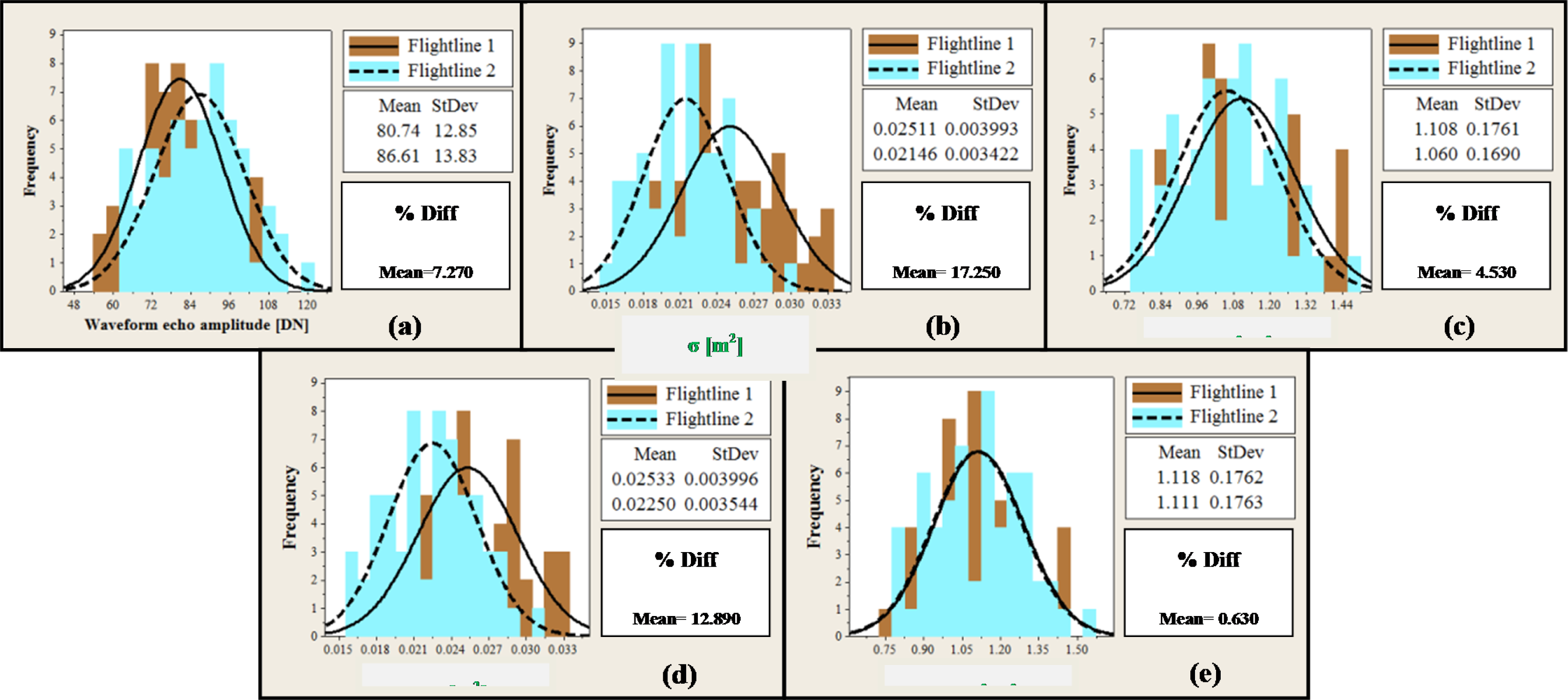
The developed technique was applied to the individual road targets, allowing determination of σ, γ, σα, and γα for each echo from both flightlines. Then, for each backscatter parameter, the values from the overlapping flightlines were compared, with results shown in Figure 3. The percentage difference statistics, which reflect the agreement of the flightline mean and standard deviation values before and after calibration show a notable improvement in the case of Figure 3c (γ) over the original amplitude signals in Figure 3a, whereas the results from σ (Figure 3b) show a deterioration. The degradation in the σ results was not expected and may be due to differences in target characteristics between flightlines. However, the γ parameter shows encouraging results as the differences are markedly reduced in comparison with the original signals.
The results for σα (Figure 3d) show a reduction in the mean and standard deviation differences as compared with σ in Figure 3b. However, the results of γα deliver a near-perfect match between overlapping flightlines, as highlighted in Figure 3e and demonstrated through small mean and standard deviation differences. Although the target was selected to be as horizontal as possible, it seems that it is not a perfectly flat surface and the incidence angle is still affecting the received signals as demonstrated by Figure 3d and Figure 3e. It is evident that the results of γα provide best agreement with the assumption made when initially selecting this target—i.e., similar conditions (e.g., range and scan angle) from both flightlines.
In seeking to deliver a comprehensive and quantitative conclusion about the optimal backscatter configuration to eliminate discrepancies between overlapping flightlines for individual feature targets, 26 different targets, encompassing a range of features and land-cover types, were identified and analysed. Each target was selected to represent a feature with homogeneous characteristics, and was composed of numerous individual echoes. These targets were grouped into six different categories with results presented in Table 3 by means of coefficient of variation (CV) statistical differences between the backscatter signals from overlapping flightlines signals before and after calibration. Amplitude represents the signal before calibration and backscatter parameters represent the signal after calibration. The mean CV was estimated for each category based on CV values delivered for each target in individual flightlines then the difference between the mean values of CV was calculated between flightlines per category. The results delivered from Table 3 indicate marked improvements after calibration with all backscatter parameters in comparison with the original amplitude differences. The γα parameter delivers the optimal match between flightlines except over the tree category, where the σ parameter shows better performance.
With the exception of the tree category, the outcomes of the backscatter parameters highlight the value of accounting for the incidence angle. In the case of trees, it is likely that an unreliable estimation of incidence angle is delivered due to the highly variable local geometry of tree echoes and thus unreliable results from the γα parameter may arise. This is evidenced through the relatively poor results achieved through σα and γα in this particular category. However, γα provides the optimal agreement between overlapping flightline signals over all other categories including short mown grass and hedges, as evidenced by the small value of the coefficient of variation differences between flightlines as demonstrated in Table 3.
5.2. Evaluating the Segmentation Routine
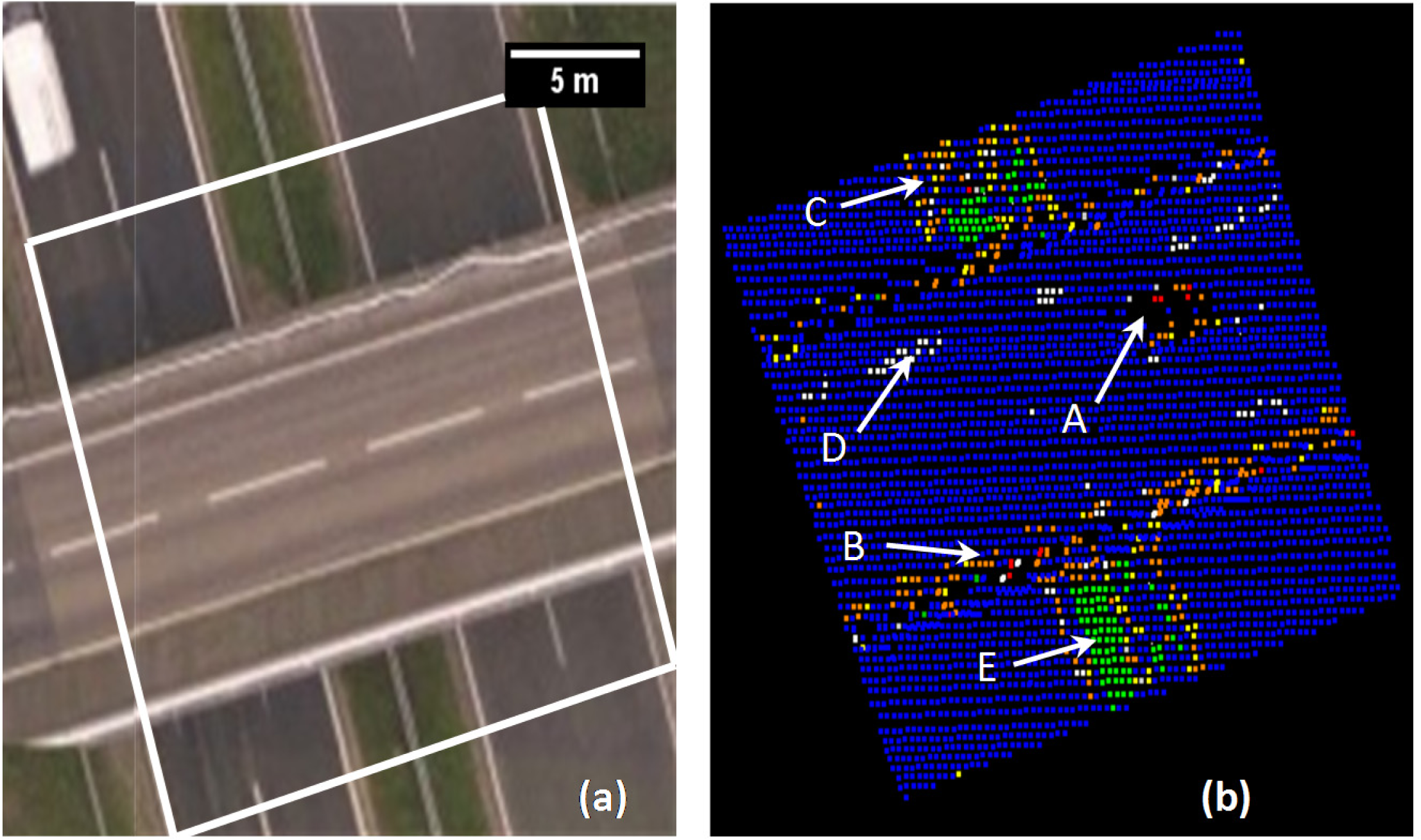
The extended test area covers more than 16 km2 and multiple targets from different regions with various physical properties were selected to test the developed segmentation routine. An example segmentation output is presented in Figure 4, which illustrates interesting results for a road bridge thatincludes various different materials such as asphalt, metal, and grass. It is evident from the segmented point cloud in Figure 4b that a car (labelled “A” in Figure 4b) was captured during the scanning, but this was not present at the instant of image acquisition (Figure 4a). The segmentation routine showed successful detection of the bridge barriers (B) on both sides of the carriageway, as well as the central reservation (C) between the two carriageways on the lower road level. Additionally, the method showed promising results in detecting some of the road markings (D) (represented in white). Figure 4 also exhibits successful segmentation of the grass regions (E) beneath the bridge (represented in green). However, a small number of echoes appear to have been wrongly segmented—possibly due to non-homogeneous properties of target materials (e.g., area around C).
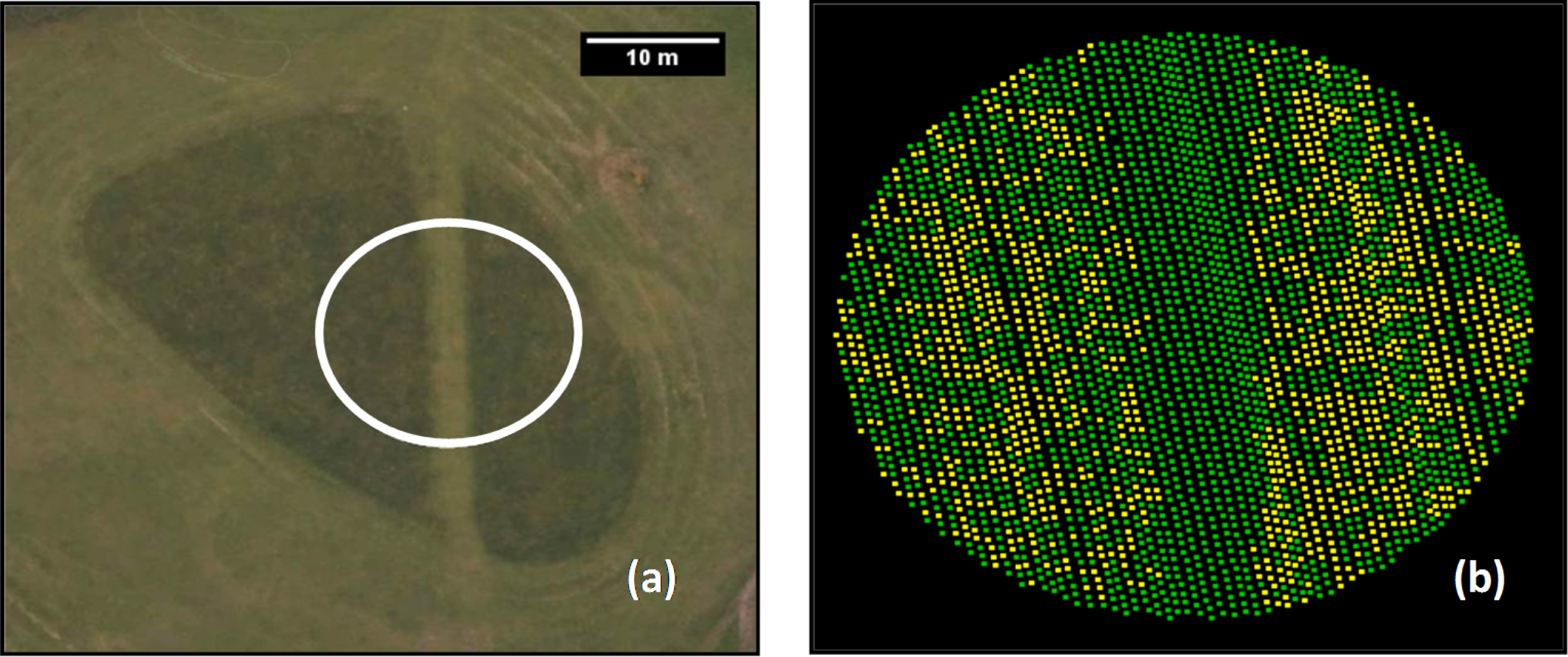
The method also shows promising results over grass regions, as illustrated in Figure 5, where two types of mown grass were successfully discriminated. The results demonstrate the method’s performance in distinguishing between two types of well-cut grass regions where both seems to have similar geometric characteristics, but different backscatter values, thus enabling their differentiation.
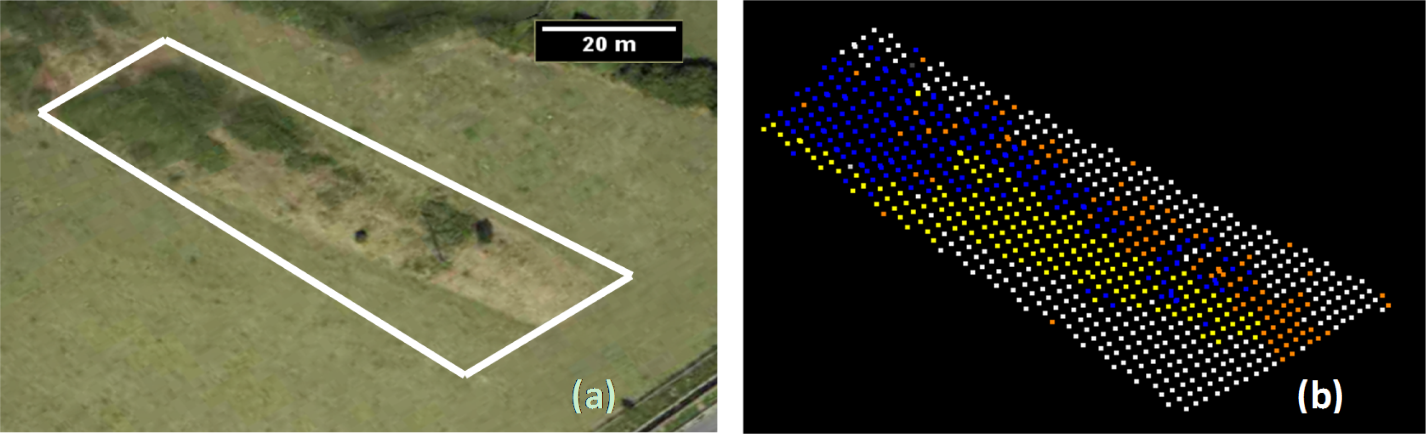
Another example is presented in Figure 6, illustrating a natural terrain target comprising a mound of earth with clumps of vegetation and grass. This demonstrates the performance of the developed method over non-planar surfaces such as natural land coverage which are likely to be partly covered by vegetation. The results show successful detection of the small mound (yellow and orange points that reflect the left and the right sides of the mound due to different orientation/slope) and differentiate this from the semi-flat surrounding ground (white points). Furthermore, the method can distinguish between both sides of the mound and also detect the vegetation patches (blue points) in the upper left corner of the figure.
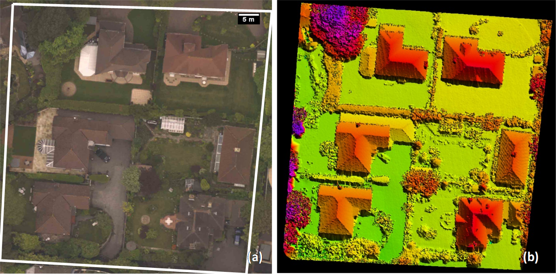
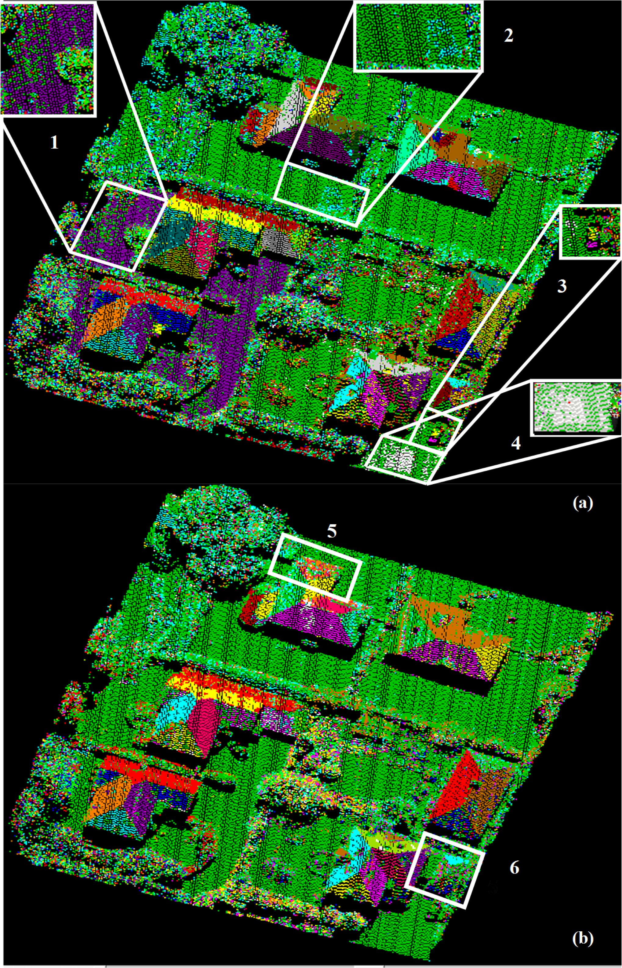
In order to examine the outcomes in more detail, a complex interest area was selected. This included various land-cover features over a residential neighbourhood area of 65 m × 65 m, as visualised in Figure 7a. The area was selected because it included a range of different land-cover types and combination of man-made, natural and semi-natural features. Figure 7b shows the digital surface model (DSM) of the selected area rendered by height differences. The segmentation results are presented in Figure 8a where some notable outcomes are highlighted. Note that, due to limitations in the colour palette range available for Figure 8a, some segments of different materials/geometry are rendered using the same colour. For example, the purple ground segments and purple roof facets are different.
The most interesting outcome from the implemented segmentation approach is the capability to discriminate grass from artificial ground (e.g., asphalt). This can be visualised clearly from the purple segment on the lower left part of the interest area. This segment was delivered after successful separation from the green grass segment that covered most of the remaining ground surface of the interest area. This can be further visualised in the highlighted inset regions of 1, 2 and 4. The method also distinguished some artificial ground echoes (light blue) from an adjacent grass segment (green), as shown in region 2, which included a concrete patio area surrounded by grass. In region 4, the method detected some asphalt echoes of the driveway area (white), but also incorrectly assigned a significant portion of what should have been asphalt echoes to the grass segment. The method also shows promise in detecting cars from the surrounding background and discriminating between different components of these minor features, such as the car’s body and roof, as illustrated in region 3. The detection of small objects such as cars is a very specific and active research topic [41,42], and although car detection was not an intended outcome of this research, the segmentation results show some potential for further investigation.
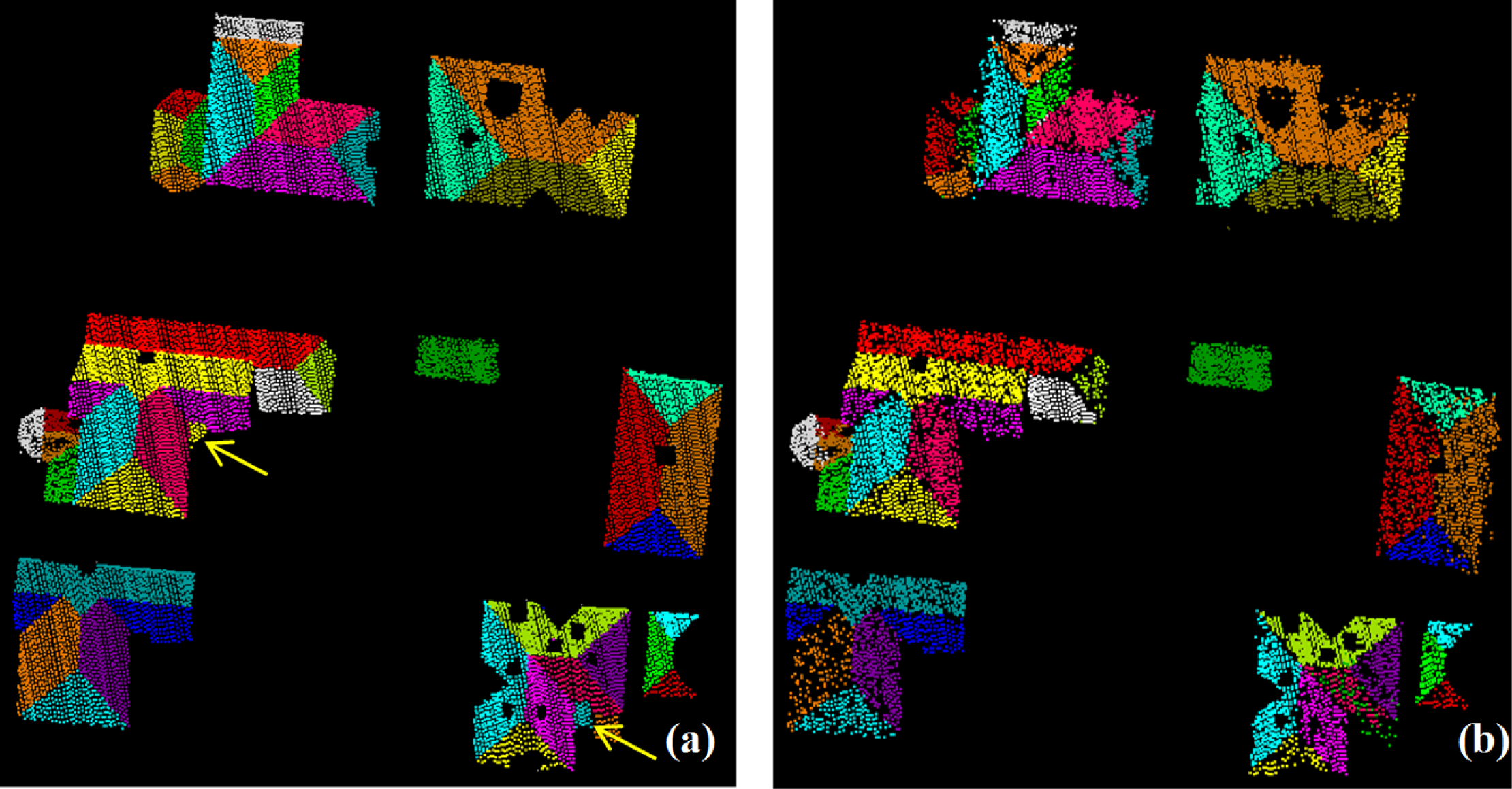
In order to analyse the potential of FWF additional information, the method was applied without integrating FWF physical observables (either in echo amplitude normalisation or in the segmentation process) for the same interest area and otherwise following the same approach. The results are demonstrated in Figure 8b. It can be seen that without FWF additional information, the method failed to discriminate grass from artificial ground. It also failed to deliver meaningful segments for car targets and demonstrated shortcomings in segmenting some roof facets with similar geometric characteristics (same height and slope) but belonging to different surfaces, as highlighted in region 5. The approach also showed poor performance over some roof surfaces where vegetation was found to cover some facets of the roof. In this case, meaningless segments were delivered, such as the example highlighted in region 6. For the same highlighted region, it can also be noticed that over some house roof facets, the integration of FWF additional information delivered more homogeneous segments than those produced without using this information. This behaviour is worth emphasising, as it demonstrates that the RSN method for determining local incidence angle [36], and subsequent incorporation into the segmentation routine, is not overlysensitive to discontinuities.
5.3. Validating the Segmentation Routine
The performance of the segmentation routine was validated by comparison to a manual segmentation process. The interest area introduced in Section 5.2 was utilised in the validation process. For accuracy assessment, an error (confusion) matrix [43] was produced. This was determined after excluding all vegetation segments (except mown grass), as it was difficult to assess performance and accuracy over these irregular features which did not conform to the regular geometric basis underpinning the implemented segmentation routine. Firstly, the interest area was segmented manually into 193 different segments using the orthophoto as a visual reference. These segments included: house roof facets; minor details over the roofs such as dormer windows and chimneys; cars; artificial ground; and mown grass. In order to visualise the performance of the introduced routine in comparison with the manual results, only house roof segments were considered, as illustrated in Figure 9.
It can be seen that the overall performance of the automatic routine is promising, as all segments were correctly determined, with the exception of a couple of minor facets in the lower-right and left-middle of the area (highlighted). Apart from this, the automatic method effectively defined the shape of individual segments by correctly distinguishing the different surfaces and geometries.
The error matrix is normally used to assess classification accuracy (in percentage terms) through the user’s accuracy and the producer’s accuracy [44]. User’s accuracy represents the error of commission as estimated based on the tested dataset, while the producer’s accuracy represents the error of omission as compared to the reference dataset. Firstly, the segments were classified into the five main classes as detailed in Table 4, to facilitate category representation in the error matrix. Thereafter, user and producer accuracies were estimated for individual categories, as illustrated in Table 5.
The user’s accuracy showed very promising results over all categories. However, slightly poorer accuracies of 75% and 76% were delivered from artificial ground and mown grass respectively. These outcomes were expected following the visual segmentation results presented in Figure 8a, which demonstrated some erroneous assignment of echoes between artificial ground and mown grass (mown grass not being a completely planar surface). This was also evident from the lower producer’s accuracy for the artificial ground category. However, high producer’s accuracy was delivered for the mown grass category. Overall accuracy (the sum of diagonal values divided by the total sum) and mean accuracy (the mean of producer’s accuracy) were estimated using the error matrix results. The overall accuracy was found to be 82% while the mean accuracy was 79%, and in both cases, these outcomes can be considered as extremely promising. Additionally, in order to compare these outcomes to the geometry-only segmentation approach, the same validation analysis was performed and a new error matrix was delivered (Table 6).
Comparison of results presented in Tables 5 and 6 illustrates deterioration in the user’s accuracy for the mown grass category. A particularly poor producer’s accuracy of 25% was obtained over artificial ground, confirming the erroneous segmentation results illustrated for such regions in Figure 8b. The segmentation accuracies (both user’s and producer’s) of chimneys and minor roof features were also noticeably poorer through this approach in comparison to the integrated approach presented in Table 5. Furthermore, the producer’s accuracy delivered for the car category was also poor at only 40%. A logical explanation for this particular behaviour could not be determined, although this result would seem to confirm the poor performance as visualised in Figure 8b. The overall and mean accuracies of the geometry-only segmentation were 67% and 60% respectively. These outcomes reflect the deterioration in the results without inclusion of FWF physical backscattering information in the segmentation process. Such results could not be achieved without an initial comprehensive radiometric calibration of the FWF physical information.
6. Conclusions
This paper has presented the development of an automated approach to 3D segmentation of FWF ALS data. The research has focussed on the calibration of the additional information from FWF ALS data, and demonstrated the novel integration of this information in a 3D object segmentation methodology. The outcomes show genuine potential for enhancing a range of downstream applications such as city modelling and topographic mapping. The method utilised FWF ALS information to overcome weaknesses in existing segmentation approaches, and to aid in discriminating between surface features with similar geometric characteristics. The method uses calibrated FWF ALS backscatter signals as a weighting function for individual echoes to estimate improved segmentation criteria. Thereafter, a surface growing approach is implemented to segment the 3D point cloud into meaningful groups. The presented technique is dependent on the reliability of the radiometric calibration routine and particularly on the robustness of the incidence angle estimation delivered from the RSN method introduced previously.
The radiometric calibration methodology considers all variables affecting the backscattered signal in the calibration process in order to deliver a more appropriate, normalised signal for downstream applications. This is achieved by considering the signal variation due to different target characteristics and accounting for variations in incidence angle. The approach demonstrated that the γα parameter provided the greatest potential amongst the four investigated backscatter parameters (σ, γ, σα, γα) by delivering an optimal match between flightlines, except over vegetation, where σ was found to produce better results.
The developed segmentation technique was assessed over selected surface features within a test dataset. The results were promising and distinctive, particularly for targets of similar geometric properties. Although some shortcomings wereidentified, for example in Figure 4 where the method failed to discriminate between the bridge surface and the underlying road surface (a shortcoming in the majority of available segmentation approaches), this could be overcome in future by incorporating height difference as an additional segmentation criterion.
Furthermore, an interest area was used to validate the segmentation by comparing results to those achieved through a manual segmentation. The process was successful and the results extremely promising with high accuracy. However, as exemplified in Figure 9, a number of points were not classified bythe automatic process and this resulted in gaps in the presented results. This can potentially be improved in future work by integrating local planarity into the segmentation process. To demonstrate the improvement delivered with integration of FWF physical observables, results were compared to those achieved through the same approach, but without inclusion of FWI information (i.e., geometry-only). The results have confirmed the potential of the FWF additional observables for improving the performance of feature segmentation. Validation against manual segmentation results confirmed a successful automated implementation, achieving an overall accuracy of 82%.
Acknowledgments
The authors gratefully acknowledge Ordnance Survey for the provision of datasets used in this research.
Author Contributions
Fanar M. Abed undertook the research which is reported in this paper as part of her PhD studies at Newcastle University. This included original development of the RSN method and all other aspects including development and implementation of the calibration and segmentation algorithms. She also carried out the bulk of the manuscript preparation.
Jon P. Mills supervised Abed’s PhD research and guided the research development. He led earlier full waveform research at Newcastle, which underpins the work reported herein. Mills contributed to the development and refinement of the manuscript.
Pauline E. Miller co-supervised Abed’s PhD and guided development of the research as the work developed. She contributed to the development and refinement of the manuscript.
Conflicts of Interest
The authors declare no conflict of interest.
References
- Shan, J.; Toth, C.K. Topographic Laser Ranging and Scanning—Principles and Processing; Taylor & Francis: Boca Raton, FL, USA, 2009. [Google Scholar]
- Vosselman, G.; Maas, H.-G. Airborne and Terrestrial Laser Scanning; Whittles Publishing: Scotland, UK, 2010. [Google Scholar]
- Lin, Y.-C.; Mills, J.P. Integration of full-waveform information into the airborne laser scanning data filtering process. Int.Arch. Photogramm. Remote Sens. Spat. Inf. Sci. 2009, 38, 224–229. [Google Scholar]
- Awwad, T.M.; Zhu, Q.; Du, Z.; Zhang, Y. An improved segmentation approach for planar surfaces from unstructured 3D point clouds. Photogramm. Rec. 2010, 25, 5–23. [Google Scholar]
- Reitberger, J.; Schnorr, C.; Krzystek, P.; Stilla, U. 3D segmentation of single trees exploiting full waveform lidar data. ISPRS J. Photogramm. Remote Sens. 2009, 64, 561–574. [Google Scholar]
- Rabbani, T. Automatic Reconstruction of Industrial Installations Using Point Clouds and Images. Ph.D. Thesis, Delft University of Technology, Stevinweg, The Netherlands,. 2006, 154. [Google Scholar]
- Filin, S.; Pfeifer, N. Segmentation of airborne laser scanning data using a slope adaptive neighbourhood. ISPRS J. Photogramm. Remote Sens. 2006, 60, 71–80. [Google Scholar]
- Sithole, G. Segmentation and Classification of Airborne Laser Scanning Data. PhD Thesis, Delft University of Technology, Stevinweg, The Netherlands,. 2005. [Google Scholar]
- Hӧfle, B.; Pfeifer, N. Correction of laser scanning intensity data: Data and model-driven approaches. ISPRS J. Photogramm. Remote Sens. 2007, 62, 415–433. [Google Scholar]
- Höfle, B.; Vetter, M.; Pfeifer, N.; Mandlburger, G.; Stötter, J. Water surface mapping from airborne laser scanning using signal intensity and elevation data. Earth Surf. Process. Landf. 2009, 34, 1635–1649. [Google Scholar]
- Mandlburger, G.; Pfeifer, N.; Ressl, C.; Briese, C.; Roncat, A.; Lehner, H.; Mucke, W. Algorithms and Tools for Airborne Lidar Data Processing from a Scientific Perspective. Proceedings of the European Lidar Mapping Forum (ELMF), Hague, The Netherlands, 30 November–1 December 2010; pp. 1–12.
- Heinzel, J.; Koch, B. Exploring full-waveform lidar parameters for tree species classification. Int.J. Appl. Earth Obs. Geoinf. 2010, 13, 152–160. [Google Scholar]
- Mallet, C.; Bretar, F.; Roux, M.; Soergel, U.; Heipke, C. Relevance assessment of full-waveform lidar data for urban area classification. ISPRS J. Photogramm. Remote Sens. 2011, 66, S71–S84. [Google Scholar]
- Rutzinger, M.; Hӧfle, B.; Hollaus, M.; Pfeifer, N. Object-based point cloud analysis of full-waveform airborne laser scanning data for urban vegetation classification. Sensors 2008, 8, 4505–4528. [Google Scholar]
- Gross, H.; Jutzi, B.; Thoennessen, U. Segmentation of tree regions using data of a full-waveform laser. Int. Arch. Photogramm. Remote Sens. Spat. Inf. Sci. 2007, 36, 57–62. [Google Scholar]
- Jutzi, B.; Neulist, J.; Stilla, U. Sub-pixel edge localization based on laser waveform analysis. Int. Arch. Photogramm. Remote Sens. Spat. Inf. Sci. 2005, 36, 109–114. [Google Scholar]
- Shi, J.; Malik, J. Normalised cuts and image segmentation. IEEE Trans. Pattern Anal. Mach. Intell. 2000, 22, 888–905. [Google Scholar]
- Yao, W.; Stilla, U. Mutual enhancement of weak laser pulses for point cloud enrichment based on full-waveform analysis. IEEE Trans. Geosci. Remote Sens. 2010, 48, 3571–3579. [Google Scholar]
- Alexander, C.; Tansey, K.; Kaduk, J.; Holland, D.; Tate, N.J. Backscatter coefficient as an attribute for the classification of full-waveform airborne laser scanning data in urban areas. ISPRS J. Photogramm. Remote Sens. 2010, 65, 423–432. [Google Scholar]
- Abed, F.M. Calibration of Full-Waveform Airborne Laser Scanning Data for 3D Object Segmentation. Ph.D. Thesis, Newcastle University, Newcastle upon Tyne, UK,. 2012, 227. [Google Scholar]
- Kaasalainen, S.; Pyysalo, U.; Krooks, A.; Vain, A.; Kukko, A.; Hyyppa, J.; Kaasalainen, M. Absolute radiometric calibration of ALS intensity data: Effects on accuracy and target classification. Sensors 2011, 11, 10586–10602. [Google Scholar]
- Jutzi, B.; Stilla, U. Range determination with waveform recording laser systems using a Wiener Filter. ISPRS J. Photogramm. Remote Sens. 2006, 61, 95–107. [Google Scholar]
- Hopkinson, C. The influence of flying altitude, beam divergence, and pulse repetition frequency on laser pulse return intensity and canopy frequency distribution. Can. J. Remote Sens. 2007, 33, 312–324. [Google Scholar]
- Höfle, B.; Hollaus, M.; Hagenauer, J. Urban vegetation detection using radiometrically calibrated small-footprint full-waveform airborne lidar data. ISPRS J. Photogramm. Remote Sens. 2012, 67, 134–147. [Google Scholar]
- Habib, A.F.; Kersting, A.P.; Shaker, A.; Yan, W.Y. Geometric calibration and radiometric correction of lidar data and their impact on the quality of derived products. Sensors 2011, 11, 9069–9097. [Google Scholar]
- Kaasalainen, S.; Ahokas, E.; Hyyppa, J.; Suomalainen, J. Study of surface brightness from backscatter laser intensity: Calibration of laser data. IEEE Geosci. Remote Sens.Lett. 2005, 2, 255–259. [Google Scholar]
- Coren, F.; Sterzai, P. Radiometric correction in laser scanning. Int. J. Remote Sens. 2006, 27, 3097–3104. [Google Scholar]
- Jelalian, A.V. Laser Radar Systems; Artech House: London, UK/Boston, MA, USA, 1992. [Google Scholar]
- Lin, Y.-C.; Mills, J.P.; Smith-Voysey, S. Rigorous pulse detection from full-waveform airborne laser scanning data. Int. J. Remote Sens. 2010, 31, 1303–1324. [Google Scholar]
- Wagner, W. Radiometric calibration of small-footprint full-waveform airborne laser scanner measurements: Basic physical concepts. ISPRS J. Photogramm. Remote Sens. 2010, 65, 505–513. [Google Scholar]
- Briese, C.; Hӧfle, B.; Lehner, H.; Wagner, W.; Pfennigbauer, M.; Ullrich, A. Calibration of full-waveform airborne laser scanning data for object classification. Proc.SPIE 2008, 6950. [Google Scholar] [CrossRef]
- Wagner, W.; Hollaus, M.; Briese, C.; Ducic, V. 3D vegetation mapping using small-footprint full-waveform airborne laser scanners. Int.Arch. Photogramm. Remote Sens. Spat. Inf. Sci. 2008, 29, 1433–1452. [Google Scholar]
- Lehner, H.; Briese, C. Radiometric calibration of full-waveform airborne laser scanning data based on natural surfaces. Int. Arch. Photogramm. Remote Sens. Spat. Inf. Sci. 2010, 38, 360–365. [Google Scholar]
- Wagner, W.; Hyyppa, J.; Ullrich, A.; Lehner, H.; Briese, C.; Kaasalainen, S. Radiometric calibration of full-waveform small-footprint airborne laser scanners. Int. Arch. Photogramm. Remote Sens. Spat. Inf. Sci. 2008, 37, 163–168. [Google Scholar]
- Airborne Laser Scanner for Full-waveform Analysis. Available online: http://www.riegl.com/uploads/tx_pxpriegldownloads/10_DataSheet_Q560_20--09--2010_01.pdf (accessed on 20 September 2010).
- Abed, F.M.; Mills, J.P.; Miller, P.E. Echo amplitude normalisation of full-waveform airborne laser scanning data based on robust incidence angle estimation. IEEE Trans. Geosci. Remote Sens. 2012, 50, 2910–2918. [Google Scholar]
- Kim, I.I.; McArthur, B.; Eric, K. Comparison of Laser Beam Propagation at 785 nm and 1550 nm in Fog and Haze for Optical Wireless Communications. Proceedings of SPIE-Optical Wireless Communications III, Boston, MA, USA, 5 November 2000; pp. 26–37.
- Doneus, M.; Briese, C. Digital Terrain Modelling for Archaeological Interpretation within Forested Areas Using Full-Waveform Laser Scanning. Proceedings of the 7th International Symposium on Virtual Reality, Archaeology and Cultural Heritage, Nicosia, Cyprus; 2006, pp. 155–162. Available online: http://luftbildarchiv.univie.ac.at/uploads/media/doneus_briese_155-162.pdf (accessed on 28 April 2014). [Google Scholar]
- Lin, Y.-C.; Mills, J.P. Factors influencing pulse width of small footprint, full waveform airborne laser scanning data. Photogramm. Eng. Remote Sens. 2010, 76, 49–59. [Google Scholar]
- Jutzi, B.; Gross, H. Investigations on surface reflection models for intensity normalisation in airborne laser scanning (ALS) data. Photogramm. Eng. Remote Sens. 2010, 76, 1051–1060. [Google Scholar]
- Yao, W.; Stilla, U. Comparison of two methods for vehicle extraction from airborne LiDAR data toward motion analysis. IEEE Trans.Geosci. Remote Sens. Lett. 2011, 8, 607–611. [Google Scholar]
- Yao, W.; Hinz, S.; Stilla, U. Extraction of motion estimation of vehicles in single-pass airborne LiDAR data towards urban traffic analysis. ISPRS J. Photogramm. Remote Sens. 2011, 66, 260–271. [Google Scholar]
- Campbell, J.B. Introduction to Remote Sensing; Taylor and Francis: London, UK, 1996. [Google Scholar]
- Congalton, R.G. A review of assessing the accuracy of classifications of remotely sensed data. Remote Sens. Environ. 1991, 37, 35–46. [Google Scholar]


| Feature Type | No. of Points | Height above Ground (m) | Mean of the Pulse Width (ns) | StDev. of the Pulse Width (ns) |
|---|---|---|---|---|
| House roof | 3198 | 3.0–6.0 | 2.557 | 0.015 |
| Mown grass | 3348 | 0.0–0.1 | 2.555 | 0.079 |
| Asphalt road | 385 | 0.0 | 2.626 | 0.028 |
| Bare natural slope | 648 | 0.0 | 2.701 | 0.055 |
| Undulating terrain | 2722 | 0.0 | 2.769 | 0.066 |
| Hedge | 533 | 0.5–2.5 | 2.599 | 0.053 |
| Scrub | 568 | 1.0–1.2 | 2.754 | 0.242 |
| Small tree | 3361 | 1.5–2.0 | 3.864 | 0.588 |
| Canopy | 6202 | 12.0–17.0 | 3.004 | 0.652 |
| Input:Pi = (X, Y, Z, N, ɸ, Ω),ɸth, δ, |
| initial region list {R} = 0, |
| available points list {A} = (1, …., Pn), |
| --------------------------------------------------- |
| While {A} ≠ 0 do |
| Current region {Rc} =0, |
| Current seed {Sc} =0, |
| Point with min. ɸ in {A} → Pmin, |
| Insert Pmin → {Sc} & {Rc}, Remove Pmin from {A}, |
| For i=0: size {Sc} |
| Find nearest neighbours of current seed point Ω(Sc(i)) → {Bc}, |
| For j=0: size {Bc} |
| Current neighbour point Bc(i) → P(j), |
| If {A} contains P(j) and |N{Sc(i)}.N{P(j)}| > cos (δ) |
| Insert P(j) → {Rc}, |
| Remove P(j) from {A}, |
| If ɸ {P(j)} < ɸth |
| Insert P(j) → {Sc}, |
| End |
| End |
| End |
| Add current region to global region, |
| Insert {Rc} → {R}, |
| End |
| End |
| Category | No. of Targets | No. of Points | Mean Difference of CV | |||||
|---|---|---|---|---|---|---|---|---|
| Flightline 1 | Flightline 2 | Amplitude | σ | γ | σα | γα | ||
| Asphalt | 5 | 6,260 | 5,825 | 0.032 | 0.016 | 0.011 | 0.015 | 0.007 |
| House roof | 6 | 6,434 | 6,279 | 0.045 | 0.043 | 0.022 | 0.027 | 0.011 |
| Car | 5 | 513 | 538 | 0.087 | 0.066 | 0.018 | 0.033 | 0.008 |
| Short mown grass | 3 | 4,391 | 4,407 | 0.044 | 0.041 | 0.027 | 0.034 | 0.024 |
| Hedge | 3 | 6,613 | 6,489 | 0.051 | 0.023 | 0.020 | 0.023 | 0.005 |
| Tree | 4 | 12,930 | 14,279 | 0.030 | 0.019 | 0.036 | 0.265 | 0.274 |
| Categories | No. of Segments | Symbol |
|---|---|---|
| House roof facets | 43 | H |
| Chimneys and minor roof features | 26 | CH |
| Cars | 2 | C |
| Artificial ground | 8 | AR |
| Mown grass | 8 | MG |
| Automatic Segmentation | |||||||
|---|---|---|---|---|---|---|---|
| Manual Segmentation | H | CH | C | AR | MG | Total | Producer’s Accuracy % |
| H | 11,367 | 69 | 0 | 1473 | 1890 | 14,799 | 77 |
| CH | 87 | 693 | 0 | 0 | 23 | 803 | 86 |
| C | 0 | 0 | 101 | 43 | 0 | 144 | 70 |
| AR | 343 | 0 | 19 | 4880 | 1962 | 7204 | 68 |
| MG | 364 | 0 | 0 | 126 | 12,099 | 12,589 | 96 |
| Total | 12,161 | 762 | 120 | 6522 | 15,974 | 35,539 | |
| User’s accuracy % | 93 | 91 | 84 | 75 | 76 | ||
| Automatic Segmentation without FWF | |||||||
|---|---|---|---|---|---|---|---|
| Manual Segmentation | H | CH | C | AR | MG | Total | Producer’s Accuracy % |
| H | 10,452 | 162 | 0 | 54 | 4131 | 14,799 | 71 |
| CH | 56 | 611 | 0 | 0 | 136 | 803 | 76 |
| C | 0 | 0 | 58 | 18 | 68 | 144 | 40 |
| AR | 0 | 0 | 0 | 1787 | 5417 | 7204 | 25 |
| MG | 809 | 200 | 11 | 580 | 10,989 | 12,589 | 87 |
| Total | 11,317 | 973 | 69 | 2439 | 20,741 | 35,539 | |
| User’s accuracy % | 92 | 63 | 84 | 73 | 53 | ||
© 2014 by the authors; licensee MDPI, Basel, Switzerland This article is an open access article distributed under the terms and conditions of the Creative Commons Attribution license (http://creativecommons.org/licenses/by/3.0/).
Share and Cite
Abed, F.M.; Mills, J.P.; Miller, P.E. Calibrated Full-Waveform Airborne Laser Scanning for 3D Object Segmentation. Remote Sens. 2014, 6, 4109-4132. https://doi.org/10.3390/rs6054109
Abed FM, Mills JP, Miller PE. Calibrated Full-Waveform Airborne Laser Scanning for 3D Object Segmentation. Remote Sensing. 2014; 6(5):4109-4132. https://doi.org/10.3390/rs6054109
Chicago/Turabian StyleAbed, Fanar M., Jon P. Mills, and Pauline E. Miller. 2014. "Calibrated Full-Waveform Airborne Laser Scanning for 3D Object Segmentation" Remote Sensing 6, no. 5: 4109-4132. https://doi.org/10.3390/rs6054109
APA StyleAbed, F. M., Mills, J. P., & Miller, P. E. (2014). Calibrated Full-Waveform Airborne Laser Scanning for 3D Object Segmentation. Remote Sensing, 6(5), 4109-4132. https://doi.org/10.3390/rs6054109