Investigating High-Resolution AMSR2 Sea Ice Concentrations during the February 2013 Fracture Event in the Beaufort Sea

Abstract
: Leads with a length on the order of 1000 km occurred in the Beaufort Sea in February 2013. These leads can be observed in Moderate Resolution Imaging Spectroradiometer (MODIS) images under predominantly clear sky conditions. Sea ice concentrations (SIC) derived from the Advanced Microwave Scanning Radiometer 2 (AMSR2) using the Bootstrap (BST) algorithm fail to show the lead occurrences, as is visible in the MODIS images. In contrast, SIC derived from AMSR2 using the Arctic Radiation and Turbulence Interaction Study (ARTIST) sea ice algorithm (ASI) reveal the lead structure, due to the higher spatial resolution possible when using 89-GHz channel data. The ASI SIC are calculated from brightness temperatures interpolated on three different grids with resolutions of 3.125 km (ASI-3k), 6.25 km (ASI-6k) and 12.5 km (ASI-12k) to investigate the effect of the spatial resolution. Single-swath data is used to study the effect of temporal sampling in comparison to daily averages. For a region of interest in the Beaufort Sea, BST and ASI-3k show area-averaged SIC of 97% ± 0.7% and 93% ± 7.0%, respectively. For ASI-6k, the area-averaged SIC are similar to ASI-3k, while ASI-12k data show more agreement with BST. Visual comparison with MODIS True Color imagery exhibits good agreement with ASI-3k. In particular, ASI-3k are able to reproduce lead structure and size in the sea ice cover, which are not or are less visible in the other SIC data. The results will be valuable for selecting a SIC data product for studies of the interaction between ocean, ice, and atmosphere in the polar regions.1. Introduction
The polar regions are essential components of the global climate system. The Arctic and Antarctic sea ice cover have considerable effects on ocean-atmosphere heat transfer [1] and on the formation of deep water masses [2]. The albedo of the polar ice cover is crucial for the global heat balance of the Earth’s climate [3]. During the last three decades, the use of remote sensing products to understand key processes in the global climate system has substantially increased [4]. For instance, sea ice concentrations (SIC) are used for investigations in climate research and for data assimilation in Numerical Weather Prediction [5,6]. Additionally, changes in sea ice extent have large impacts on the Arctic climate system, e.g., the connection of and interaction between sea ice, air temperature and permafrost on continents and ocean shelves is a matter of current research [7]. Since the 1970s, numerous satellite missions have been launched and a considerable number of algorithms has been developed to derive SIC from passive-microwave (PM) data. These algorithms use approximations of the radiative transfer equation for electromagnetic waves in the microwave regime, empirical approaches that consider relationships between brightness temperatures (Tb) and SIC, or a combination of both [8].
In the course of the “Arctic Radiation and Turbulence Interaction Study” (ARTIST), the ARTIST sea ice algorithm (ASI) was developed using the 85-GHz channels of the Special Sensor Microwave/Imager (SSM/I) to provide high spatial resolution SIC [9]. The algorithm is based on the Svendsen sea ice algorithm for near-90-GHz frequencies [10]. With the start of NASA’s Advanced Microwave Scanning Radiometer (AMSR-E) on-board the Aqua satellite, the spatial resolution at 89-GHz became nearly three times higher than for SSM/I at 85-GHz [11]. Consequently, the ASI algorithm was adapted for the use of 89-GHz measurements [11]. Despite the enhanced sensitivity to the atmospheric influence at these frequencies compared to lower microwave frequencies, this algorithm provides almost weather-independent SIC [9,11]. A detailed description and derivation of the algorithm and the weather filtering can be found in Kaleschke et al. (2001) [9] and Spreen et al. (2008) [11].
AMSR-E-based ASI SIC provide a horizontal resolution that is up to four times higher than another algorithm that is widely used to retrieve SIC, the Bootstrap algorithm [12–14]. The Bootstrap algorithm (BST) mainly utilizes the Tb measured at the frequencies of 18.7- and 36.5-GHz and, therefore, depends on a larger footprint size of the measured Tb data, which reduces the spatial resolution of the retrieved SIC. With the launch of the Japan Aerospace Exploration Agency’s (JAXA) Advanced Microwave Scanning Radiometer 2 (AMSR2), the improved successor of AMSR-E, the spatial resolution of ASI SIC has even further improved, due to both scans available from the feedhorns measuring at 89-GHz.
This work studies the effect of spatial resolution and temporal sampling in ASI SIC on the ability to resolve local structures, like leads within the sea ice cover. Leads are large, elongated or linear-like fractures in a formerly solid sea ice cover that develop due to divergence and shear forces within the sea ice cover [15]. Through uncovering the relatively warmer ocean surface to the cold winter atmosphere, leads are of significant importance for the local near-surface heat balance of the winter Arctic atmosphere [15]. From a modeling study of atmosphere-ocean heat exchange due to lead openings, it is inferred that a change in SIC of 1% can cause a near-surface temperature increase of up to 3.5 K [16].
The paper proceeds in the following way: Section 2 briefly reports new features of the AMSR2 sensors. Section 3 introduces the new 3.125-km ASI SIC and lower resolution derivatives of ASI and JAXA’s AMSR2-based SIC that are used in this study for comparison. In Section 4, we present the comparison, and we end with a discussion in Section 5.
2. AMSR2
The AMSR2 on-board the Global Change Observation Mission 1st-Water (GCOM-W1) satellite is the successor instrument of AMSR-E [17]. It was launched in May 2012 and placed into the Afternoon Constellation (A-Train) [17]. The A-Train consists of a number of Earth observing satellites that orbit the Earth in a sun-synchronous orbit in close proximity at about a 700-km height above the Earth’s surface. The constellation crosses the equator at around 1:30 P.M. mean solar time [18]. AMSR2 Level-1 Tb data are available for the period starting in July 2012 via JAXA’s GCOM-W1 Data Providing Service.
The AMSR2 instrument is a conically-scanning PM radiometer system that measures in seven frequency bands ranging between 6.925 GHz and 89.0 GHz at both horizontal and vertical polarization. The antenna’s different feedhorns scan at an incidence angle of 55°and provide a 1450-km swath width at the Earth’s surface [17]. Compared to AMSR-E, AMSR2 provides improved characteristics [17]:
The size of its main reflector has increased from 1.6 m (for AMSR-E) to 2.0 m (for AMSR2), which leads to smaller footprints and, thus, higher spatial resolutions for the different frequencies;
Its calibration system has improved, leading to higher temperature stability when calculating Tb from sensor data, due to a more homogeneously calibrated warm load—the High Temperature Noise Source (HTS); and
A redundant momentum wheel has been added to the system to increase reliability.
3. AMSR2-Based Sea Ice Concentrations
3.1. Processing of Sea Ice Concentrations Using ASI
For the new ASI AMSR2 SIC, we process single swaths of Level-1R Tb data that are based on Level-1B Tb data. In the Level-1B data, the center of a footprint at each frequency that corresponds to the same scan number or pixel can differ in its location on the Earth’s surface by several kilometers [19]. For the Level-1R data, the different channel’s footprints have been resampled to match the same location and the resolution of lower frequency channels. For that, Level-1B Tb data are recalculated using the Backus–Gilbert method (see [17,20,21]). This method improves the retrieval accuracy of higher level products, and we expect the weather filters to give more consistent results when the 18.7-GHz, the 23.8-GHz and the 36.5-GHz channels are georeferenced and Backus–Gilbert-interpolated to the same footprint location. To interpolate the satellite measurements onto a regular grid, we resample the swath-based Tb using a nearest neighbor approach. From the gridded swath-based Tb data, we calculate daily-mean Tb maps. Based on these daily-mean Tb maps, SIC are calculated, and the weather filters are applied. For single-swath SIC, the single-swath Tbs are processed accordingly without calculating daily-mean Tb maps. Then, monthly maximum-extent masks from the National Snow And Ice Data Center (NSIDC, [22]) are used to remove false SIC that may still exist over open water areas. These monthly maximum-extent masks are provided on the original 25-km grid used for the Nimbus-7 Scanning Multichannel Microwave Radiometer (SMMR) and SSM/I SIC. We interpolate these masks to the 12.5-km, 6.25-km and 3.125-km grids that are used for our data and manually correct for coarse coastlines stemming from the original 25-km resolution. Due to the long-term decline in sea ice extent and SIC [23], we consider the potential very unlikely that the used climatology cuts off sea ice outside of the masked regime. Note that the tie-points used in the AMSR2 SIC processing have not been adapted to the new sensor, and the former AMSR-E derived tie-points [11] are still used. This is a valid approach in this study, because of the similarities of the AMSR2 instrument to the AMSR-E instrument. For long-term time series analysis using data from both sensors, an adjustment would be needed. We provide ASI-AMSR2 3.125-km SIC for both hemispheres on a daily basis through the Integrated Climate Data Center (ICDC) of the University of Hamburg (see http://icdc.zmaw.de).
For this study, we also calculate ASI SIC at 6.25-km (ASI-6k) and 12.5-km (ASI-12k) resolution. ASI-6k is intended to simulate AMSR-E-based SIC by only considering 89-GHz B-scan measurements to derive SIC. The A-scan of the 89-GHz feedhorn of AMSR-E measurements started producing corrupted measurements from the period starting in November 2004. For ASI-12k, we simulate the larger footprint size of the 18-GHz channel (see Table 1) by resampling multiple 89-GHz scans within a search radius that matches the 18-GHz footprint size. The scans found within the search radius are averaged by Gaussian weighting considering the distance to the center of the search field. Then, the resampled Tb data are input to the SIC retrieval. Thereby, we investigate the effect of the larger footprint on the SIC retrieval. The 18-GHz Tb data, together with 36-GHz Tb data, provide the main ice information in the BST processing (see Section 3.2).
3.2. AMSR2 BST Sea Ice Concentrations
The ASI-based SIC are compared with SIC that are derived using the Bootstrap algorithm provided as Level-3 data by JAXA [24]. Daily-mean SIC are provided separately for ascending and descending swaths at 10-km resolution via JAXA’s GCOM-W1 Data Providing Service. We average both daily products to one daily-mean SIC map to compare with the ASI-based daily-mean SIC maps.
4. Comparison of the High-Resolution ASI SIC with MODIS Data, BST SIC and ASI SIC at Coarser Resolutions
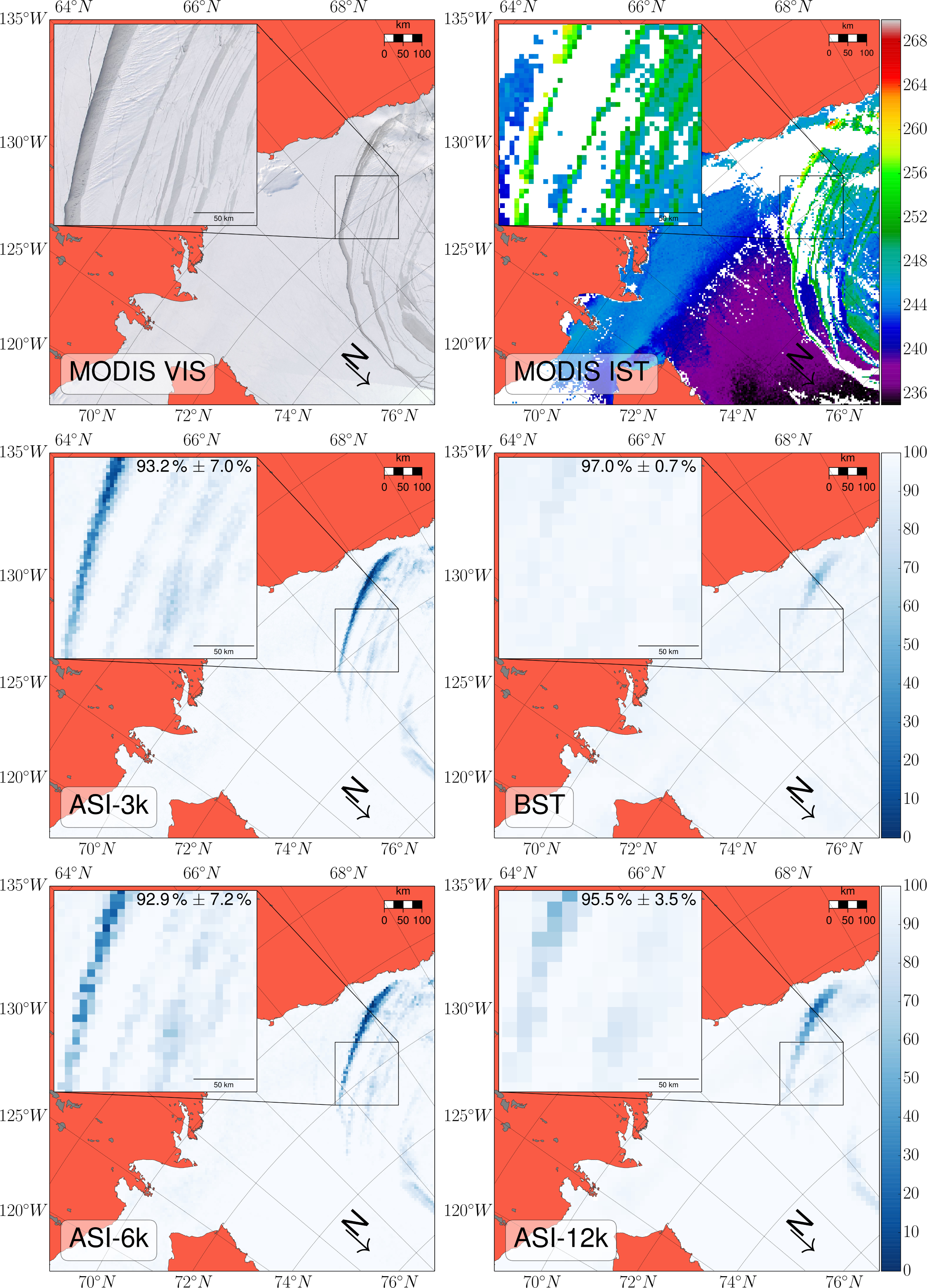
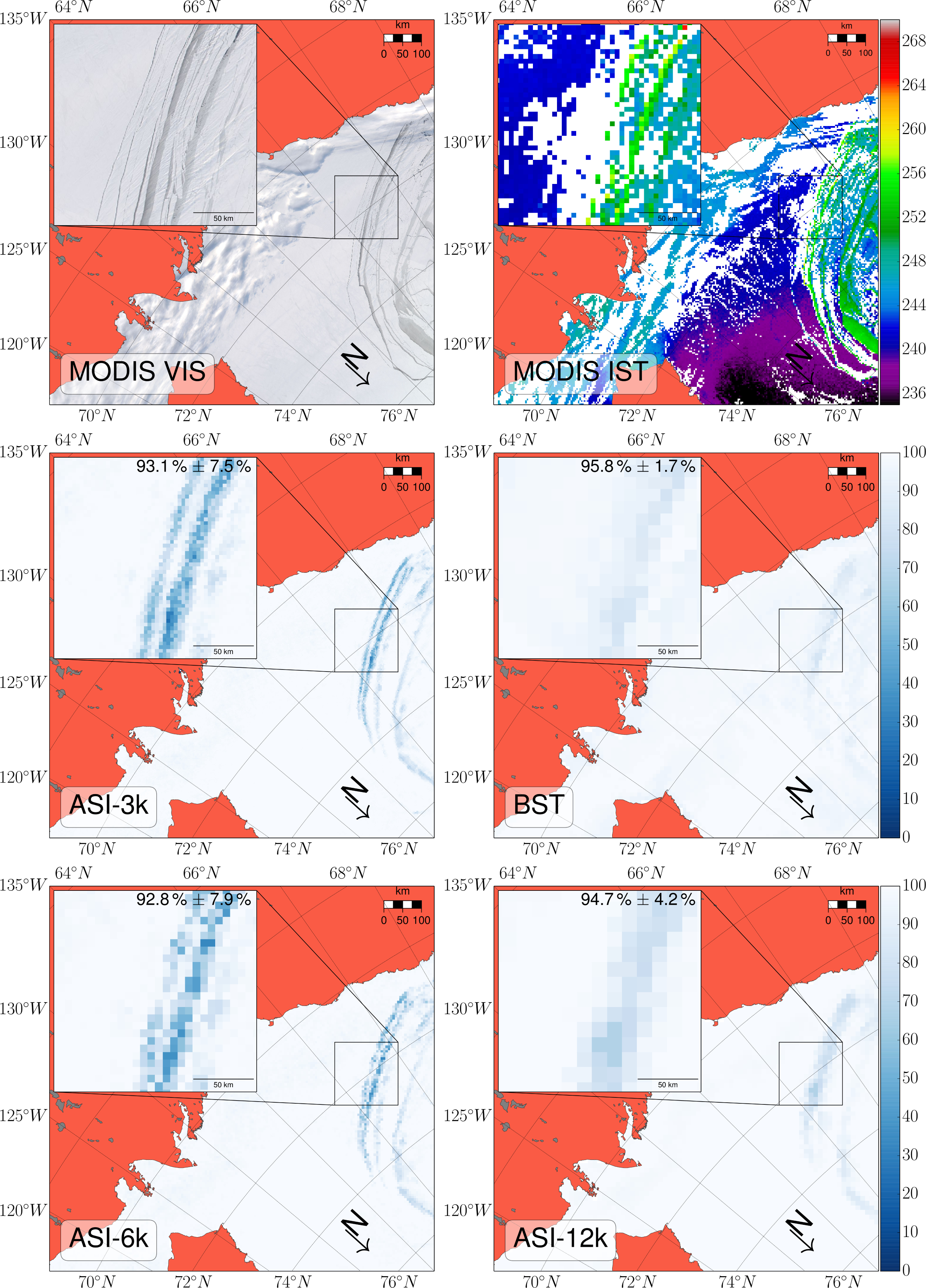
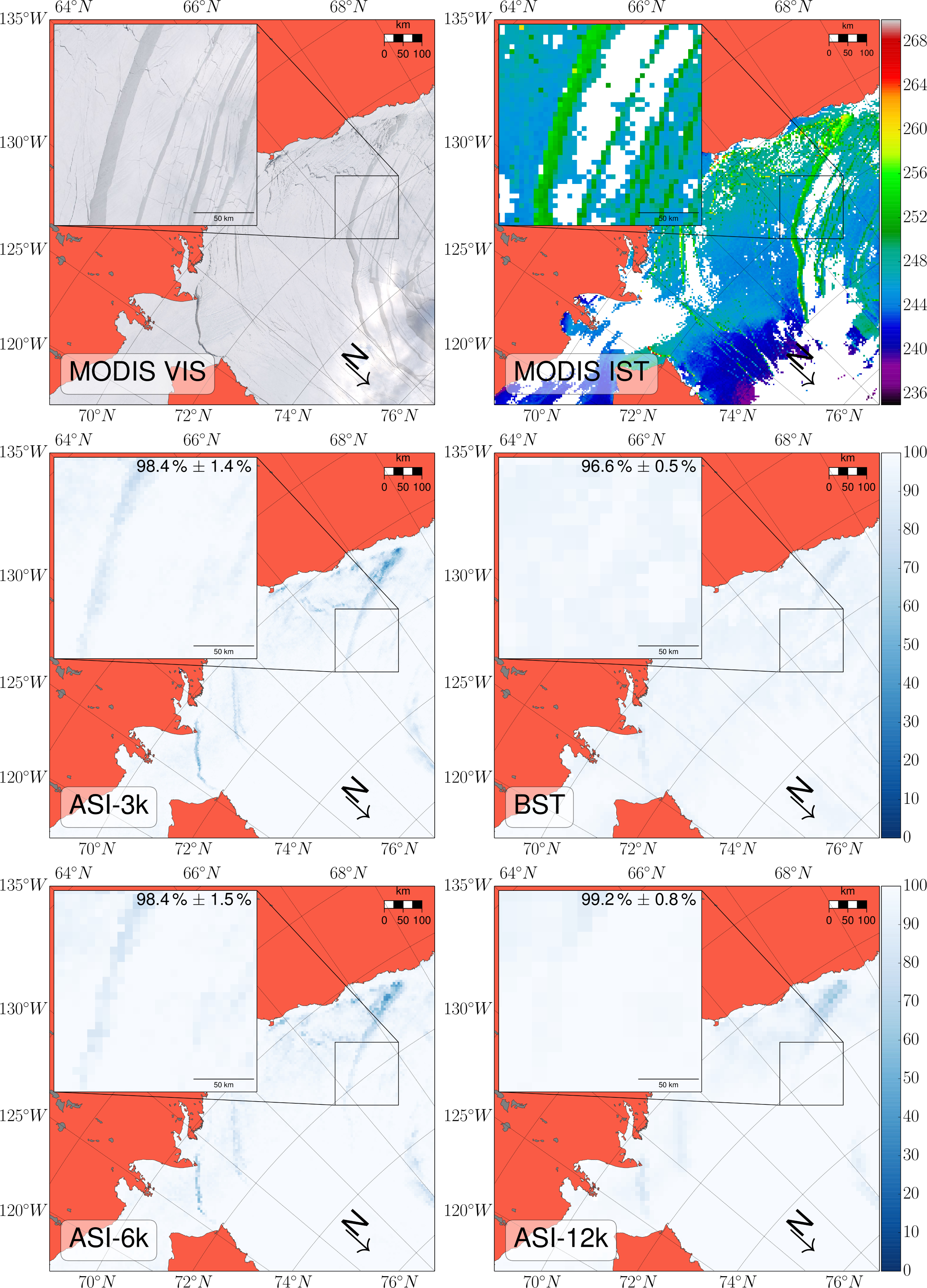
To evaluate the performance of the new high-resolution SIC, we compare ASI-3k with ASI-6k, ASI-12k and AMSR2-based BST SIC for a period in February 2013 in the Beaufort Sea. Additionally, these SIC are compared with 250-m resolution MODIS True Color (MODIS VIS) and 4-km resolution MODIS ice surface temperatures (MODIS IST) [25] (Figures 1 and 3).
All maps in Figures 1 and 3 display a part of the southern Beaufort Sea for 25, 26 and 27 February, respectively. From 21 February onwards, the sea ice cover started moving towards the Bering Strait, with several leads appearing every day in the western area shown in the maps. During the following days, progressively more leads appeared towards the Canadian Arctic Archipelago (CAA), until, on 27 February, recently formed and partly refrozen leads pervaded the sea ice cover of the whole Western Arctic. Only the land-fast ice close to the Canadian coast and the sea ice in the CAA was intact. In this study, we focus on a ∼1000 km-long lead (henceforth called Feb-26-lead) that developed between 25 February and 26 February and is located between 76° N and 135° W in the lower right part of the maps and close to the coast of Alaska, near Prudhoe Bay (approximately at 70° N and 148° W) (Figure 2).
In MODIS VIS (Figure 2), the Feb-26-lead appears as a dark opening in the otherwise bright sea ice cover. Distinct temperature differences exist between the partly open and partly refrozen areas of the Feb-26-lead and the surrounding solid ice cover, visible in the MODIS IST map. These temperature differences are 20 K maximum for the inset area. In this inset, parts of the temperature data close to the location of the Feb-26-lead have been filtered due to a cloud mask or because the surface is detected as open water. However, the structure and the position of the Feb-26-lead are recognizable. Most of the full MODIS tile is cloud free and provides clear-sky conditions enabling comparison with the different AMSR2 SIC data.
Other leads, which had formed on 25 February (see Figure 1), are located west of the Feb-26-lead and show a higher albedo, indicating a refrozen ice surface. On 26 February, the albedo in the Feb-26-lead increases from left to right (MODIS VIS, Figure 2); this suggests the presence of open water at the windward side and a new ice cover becoming progressively thicker, building up towards the leeward side. Additionally, open water patches can be identified at some locations in this new ice cover. The moisture and heat input through the openings into the atmosphere generates clouds. These clouds spread westward by the easterly winds and form cloud streets in the lee of the openings. Most of these clouds are detected by the cloud mask used in the MODIS IST data set (see the inset in MODIS IST, Figure 2). The MODIS IST data from within the Feb-26-lead suggest a mixture of open water and thin ice, but the grid resolution of 4 km is too large to adequately discriminate both surface types. The Feb-26-lead shows a higher albedo on 27 February (MODIS IST in Figure 3), indicating thickening of the new ice cover. Additionally, MODIS IST exhibits lower temperatures for the lead area (MODIS IST, Figure 3). For the solid sea ice cover, ice surface temperatures decrease with increasing latitude, mirroring the low near-surface air temperatures during the period of investigation (not shown).
The lower four panels of Figures 1 and 2 exhibit quite substantial differences among the SIC data. For the three ASI maps—ASI-12k, ASI-6k and ASI-3k—these differences result from the different grid resolutions and, therefore, from the sampling routines applied (see Section 3.1). Most details of the Feb-26-lead are visible in the ASI-3k map. In contrast, BST shows only reduced SIC for the area of the Feb-26-lead. Only close to the Alaskan coast, where the lead has its maximum width, BST SIC are as low as ∼50% SIC. The difference between BST and ASI-3k in area-averaged SIC for the zoomed area in the insets is ∼4% on 26 February (numbers are shown in the upper right corner of the individual insets for SIC data in Figures 1 and 3). In contrast, ASI-12k data look very similar to BST, suggesting that the footprints at 18 and 36 GHz are too large to resolve the Feb-26-lead. These footprint’s signatures include contributions from the nearby thick sea ice.
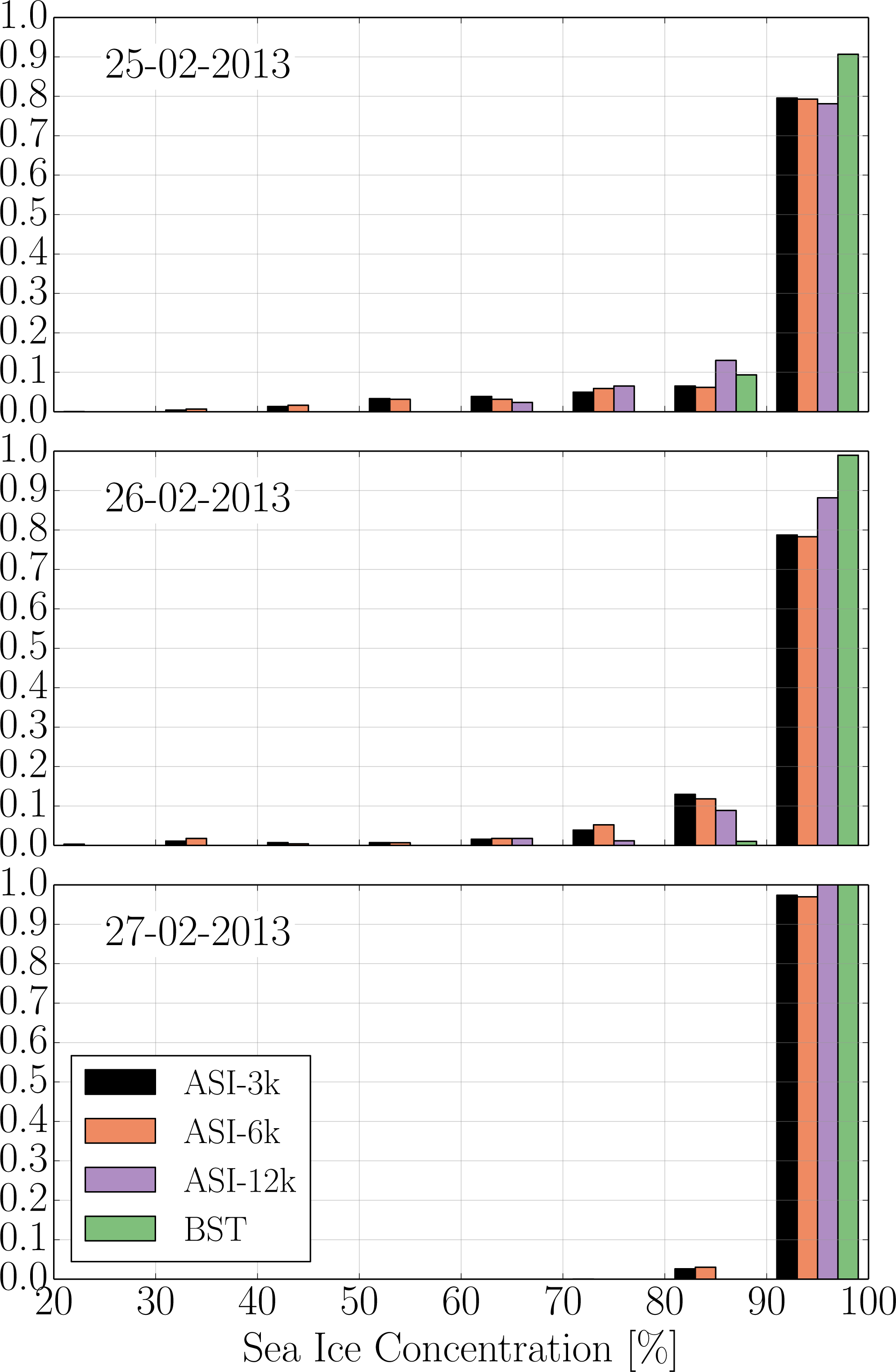
The gain of information due to the higher resolution in SIC data is shown in histograms in Figure 4. ASI-3k and ASI-6k are able to detect SIC in the range of 30%–80% on 25 February and 26 February, respectively. These low- to mid-level SIC stem from the lead, which is westward of the Feb-26-lead (see Figure 1). In the high SIC bin (>90%), all ASI-based SIC data reveal less ice than BST. ASI-12k shows the lowest relative probability in this bin due to the larger grid size, but, in contrast to ASI-3k and ASI-6k, ASI-12k is not able to detect SIC less than 60%. The differences in relative probability between ASI-3k and ASI-6k are quite small for 25–26 February. On 27 February, the area in the inset is almost completely refrozen according to the SIC data with only ASI-3k and ASI-6k displaying SIC in the 80%–90%-bin.
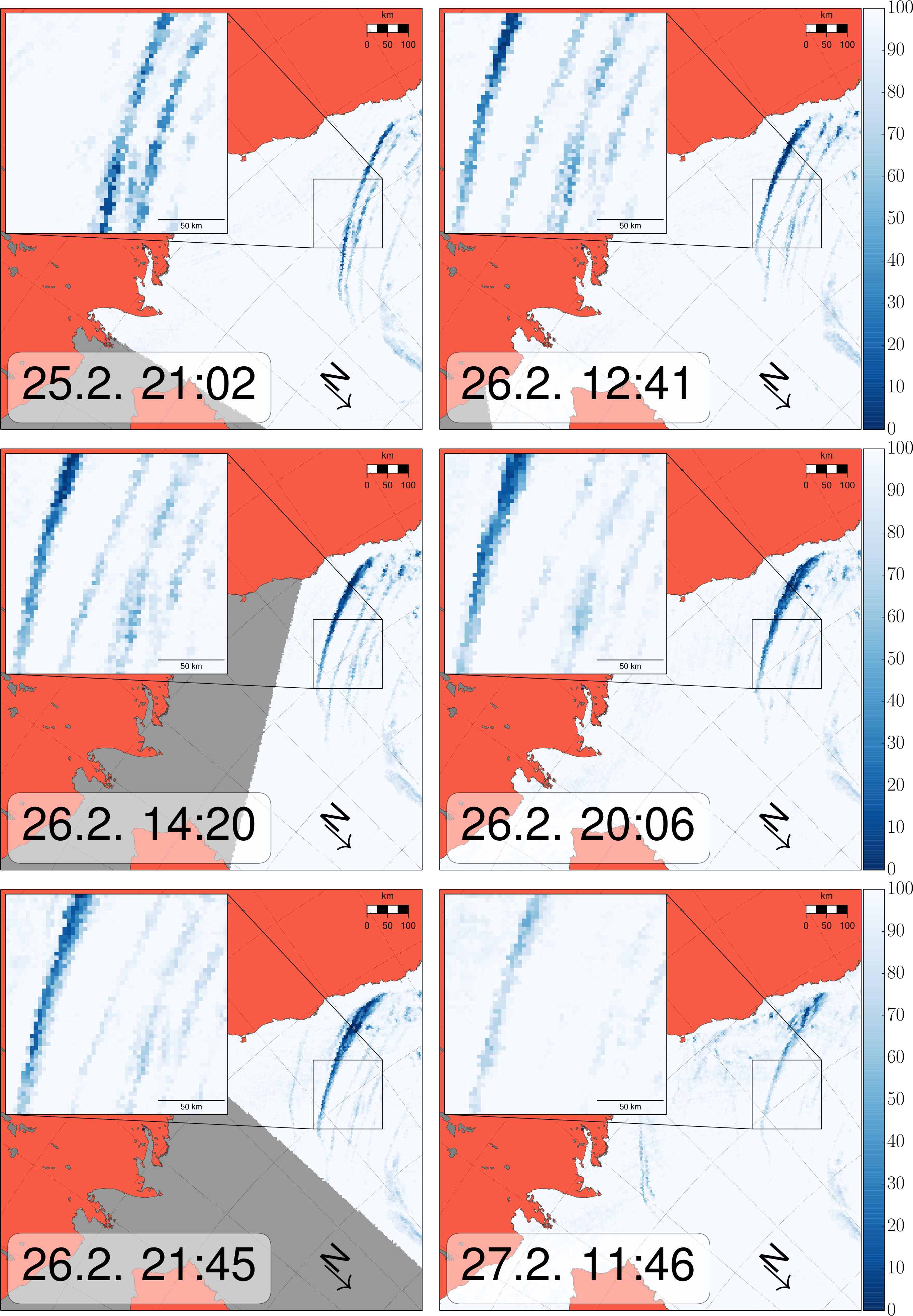
The dynamic evolution of the ice cover complicates a comparison on a daily-mean basis. Considering ASI-3k SIC retrieved from single-swath Tb data reveals more details on the development of the Feb-26-lead and its refreezing (Figure 5). The Feb-26-lead develops between 21:02 UTC on 25 February and 12:41 UTC on 26 February. The MODIS scene, which most of the tile shown (MODIS VIS, Figure 2) is based on, was recorded at 20:55 UTC. The lead shows a higher albedo and, therefore, a refrozen surface in the northern part of the image. The southern part, also partly visible in the inset, has substantial open water fractions on the windward side and within the new ice on the leeward side of the lead. We investigate the size of the Feb-26-lead in the SIC data by calculating the open water fraction of the lead separately for each of the swaths shown in Figure 5. For that, we select a region around the Feb-26-lead and generate a mask that only considers SIC values below 50% in this region based on the daily-mean ASI-3k data. Note that this analysis is based on the assumption of no drift. This would introduce an error when the lead is displaced. From 25 to 27 February, the open water fraction increases from 0% on 25 February to ∼80% on 26 February and decreases to ∼15% on 27 February. Based on this calculation, the Feb-26-lead reaches its maximum size on 26 February between the AMSR2 overflights at 14:20 UTC and 20:06 UTC.
5. Discussion
In the previous section, we presented a case study using a new 3.125-km passive-microwave sea ice concentration (SIC) data set that is calculated based on AMSR2 Level-1R brightness temperature (Tb) measurements. In November 2004, the A-scan of the 89-GHz feedhorn of AMSR-E measurements started producing corrupted data, after which these scan data had to be discarded. With AMSR2, we provide twice the resolution of the previous 6.25-km grid resolution that was used for AMSR-E.
We compared different data sets for a late winter situation when several elongated and relatively wide leads occurred in the Beaufort Sea. One of those leads, the Feb-26-lead, was on the order of 1000-km long. The ASI SIC data on a 3.125-km grid (ASI-3k) resemble the pattern of the fractured sea ice cover as it is visible in a MODIS True Color image (MODIS VIS) and the MODIS ice surface temperatures (MODIS IST). Discrepancies exist when comparing ASI-3k to JAXA’s Bootstrap-based SIC data. Bootstrap (BST) is a mature, well-validated algorithm that is known to represent local SIC very accurately [26]. In this particular case, however, BST SIC do not show the Feb-26-lead structures as they are visible in MODIS VIS, the ASI-3k, and the ASI-6k images. ASI-3k and ASI-6k show a considerable open water fraction in the southern part of the Feb-26-lead (above the inset in the maps shown). Our analysis suggests the differences to BST SIC arising from the larger footprints of the lower frequencies that are used in the BST retrieval. At these lower frequencies, the Tb signal of pixels located within the Feb-26-lead is influenced by surrounding thicker sea ice, which is characterized by much higher Tb than the open water surface and new ice in the lead. Therefore, these pixels show a temperature mix of the open water, new ice, and thick sea ice. Additionally, the microwave signal is very sensitive to the location of one measurement, i.e., the location of the footprint; this can result in large differences for the calculation of SIC if the center of a footprint is located within the open water area or if it is located at the margin of a lead with a considerable influence of the thicker sea ice surface. In the ASI-3k and ASI-6k maps, more structural details of the Feb-26-lead are visible than in the BST SIC map and in the ASI-12k data. ASI-12k simulates the larger footprint of the 18-GHz measurements that are input to the BST retrieval. This simulation confirms the disadvantage of lower-frequency-based SIC retrievals in resolving the details of lead structures during the period that we show in our case study.
We cannot determine quantitatively if and how much ASI-3k overestimates the open water in the Feb-26-lead. The east-west gradient in the albedo within the Feb-26-lead visible in the MODIS True Color maps indicates the presence of both open water and new ice. The albedo of the new ice part of the Feb-26-lead seems to suggest relatively thick new ice, like light nilas or grey ice. However, such a high albedo can also be caused by frost flowers growing on thin new ice, like dark nilas under cold conditions [27]. The existence of cloud streets advected downwind of the Feb-26-lead ensures that a substantial amount of open water existed to which the two used SIC retrieval algorithms are sensitive, provided that the achieved spatial resolution is fine enough. Only with the new ASI SIC data set with 3.125-km grid resolution, the structure, position and size of all the leads displayed in MODIS imagery shown for the tree consecutive days in February 2013 (Figures 1 and 3) are depicted correctly.
Larger uncertainties or even biases can be expected in the retrieved SIC, because the radiometric surface properties of thin ice differ from those of thick ice, whose radiometric properties determine the sea ice tie points used in the SIC algorithms. Evidence for a thin ice SIC bias have been found in a number of studies [28–31]. In the present study, emphasis is put on the occurrence and structure of the leads rather than onto a correct quantification of SIC in the lead itself. Natural variability in sea ice properties, e.g., due to snow metamorphism or ice-snow interface roughness changes, causes a variability in the retrieved SIC of a few percent [32]. This is an uncertainty high enough to make the detection of changes by 1–2% in high ice concentration areas, e.g., due to leads, impossible. In the present study, however, the short duration of the investigation period of three days and the constantly cold, dry conditions ensure minimum day-to-day variation in SIC due to the above-mentioned property changes.
Reductions in winter SIC of a few percent are known to already induce great effects in the lower atmospheric heat budget because of increased ocean-atmosphere heat exchange [15]. With a high resolution SIC data set, it is more likely to correctly detect such SIC variations and, hence, to provide the basis for a more realistic quantification of winter-time ocean-atmosphere heat exchange. The ASI-3k is able to depict smaller-scale openings in the sea ice cover and shows an open water fraction, which is 4% higher than the one from BST for our area of interest of size 170 km × 170 km in the Beaufort Sea.
6. Conclusion
In summary, we present a new high-resolution sea ice concentration data set based on satellite microwave radiometry that is able to provide more details of a fractured sea ice cover than sea ice concentration data at lower spatial resolutions. This is achieved by applying the ARTIST Sea Ice (ASI) algorithm to brightness temperatures measured at a frequency of 89-GHz by the Advanced Microwave Scanning Radiometer-2 (AMSR2). This enables to retrieve sea ice concentrations at 3.125-km grid resolution (ASI-3k SIC). The data set has the potential to provide a more realistic boundary condition when calculating atmosphere-ice-ocean exchange processes. A high-resolution SIC data set is an advantage for navigation through the sea ice cover, as well as for mesoscale process studies [9], and daily-mean ASI-3k SIC provide a high level of details about the ice pack. However, if knowledge about sea ice concentration for a specific point in time is required (e.g., for data assimilation), we recommend, based on our investigation of spatial resolution and temporal sampling, using ASI-3k SIC calculated from individual swath data if available, because more details of an ice situation for a defined time can then be obtained.
Acknowledgments
The authors acknowledge funding by the Bundesministerium für Wirtschaft und Technologie (BMWi, Federal Ministry of Economics and Technology) through the project “Ice-Route-Optimization-2” (IRO-2, U-4-6-03-BMW-11-02) in the framework of the program “Shipping and ocean engineering for the 21st century”, and funding through the Deutsche Forschungsgemeinschaft (DFG, German Research Foundation) through the Cluster of Excellence (CliSAP, EXC 117). We acknowledge the use of Rapid Response imagery from the Land Atmosphere Near-real-time Capability for EOS (LANCE) system operated by NASA’s Goddard Space Flight Center Earth Science Data and Information System (ESDIS) with funding provided by NASA Headquarters. We thank JAXA ( http://www.jaxa.jp/index_e.html) for the provision of AMSR2 data. Rein Klazes helped to reduce errors in the processing of the AMSR2 data. Monika Onken and David Bröhan provided their Python codes for plotting MODIS tiles and zooming into a data array, respectively; both of these programs were used as a starting point for the graphics shown in Figures 1 and 3 and 5. Resampling was done using Python’s pyresample ( https://pyresample.readthedocs.org/en/latest/index.html). We thank Nina Maaß, Maciej Miernecki, and Mark Carson for valuable discussions and help on the manuscript. Three anonymous reviewer helped to improve the manuscript.
Author Contributions
With the start of AMSR2, the main idea that led to this paper was developed as part of a work package within the IRO-2 project. It was intended to provide a follow-up data set of sea ice concentrations succeeding AMSR-E. Alexander Beitsch carried out the data analyses and wrote the manuscript incorporating suggestions from Stefan Kern and Lars Kaleschke. Lars Kaleschke and Stefan Kern supervised the research leading to the manuscript. All authors approved the final manuscript.
Conflicts of Interest
The authors declare no conflicts of interest.
References
- Maykut, G.A. Large-scale heat exchange and ice production in the central Arctic. J. Geophys. Res 1982, 87, 7971–7984. [Google Scholar]
- Stossel, A. Employing satellite-derived sea ice concentration to constrain upper-ocean temperature in a global ocean GCM. J. Clim 2008, 21, 4498–4513. [Google Scholar]
- Curry, J.A.; Schramm, J.L.; Ebert, E.E. Sea ice-albedo climate feedback mechanism. J. Clim 1995, 8, 240–247. [Google Scholar]
- Stroeve, J.C.; Serreze, M.C.; Holland, M.M.; Kay, J.E.; Malanik, J.; Barrett, A.P. The Arctic’s rapidly shrinking sea ice cover: A research synthesis. Clim. Chang 2012, 110, 1005–1027. [Google Scholar]
- Uotila, P.; Vihma, T.; Pezza, A.B.; Simmonds, I.; Keay, K.; Lynch, A.H. Relationships between Antarctic cyclones and surface conditions as derived from high-resolution numerical weather prediction data. J. Geophys. Res.: Atmos 2011. [Google Scholar] [CrossRef]
- Donlon, C.J.; Martin, M.; Stark, J.; Roberts-Jones, J.; Fiedler, E.; Wimmer, W. The operational sea surface temperature and sea ice analysis (OSTIA) system. Remote Sens. Environ 2012, 116, 140–158. [Google Scholar]
- Parmentier, F.J.W.; Christensen, T.R.; Sorensen, L.L.; Rysgaard, S.; McGuire, A.D.; Miller, P.A.; Walker, D.A. The impact of lower sea-ice extent on Arctic greenhouse-gas exchange. Nat. Clim. Chang 2013, 3, 195–202. [Google Scholar]
- Steffen, K.; Key, J.; Cavalieri, D.J.; Comiso, J.; Gloersen, P.; Germain, K.S.; Rubinstein, I. The Estimation of Geophysical Parameters Using Passive Microwave Algorithms. In Microwave Remote Sensing of Sea Ice; American Geophysical Union: Washington, DC, USA, 1992; pp. 201–231. [Google Scholar]
- Kaleschke, L.; Lupkes, C.; Vihma, T.; Haarpaintner, J.; Bochert, A.; Hartmann, J.; Heygster, G. SSM/I sea ice remote sensing for mesoscale ocean-atmosphere interaction analysis. Can. J. Remote Sens 2001, 27, 526–537. [Google Scholar]
- Svendsen, E.; Matzler, C.; Grenfell, T.C. A model for retrieving total sea ice concentration from a spaceborne dual-polarized passive microwave instrument operating near 90 GHz. Int. J. Remote Sens 1987, 8, 1479–1487. [Google Scholar]
- Spreen, G.; Kaleschke, L.; Heygster, G. Sea ice remote sensing using AMSR-E 89-GHz channels. J. Geophys. Res.: Ocean 2008. [Google Scholar] [CrossRef]
- Comiso, J.C.; Cavalieri, D.J.; Parkinson, C.L.; Gloersen, P. Passive microwave algorithms for sea ice concentration: A comparison of two techniques. Remote Sens. Environ 1997, 60, 357–384. [Google Scholar]
- Comiso, J.C.; Cavalieri, D.J.; Markus, T. Sea ice concentration, ice temperature, and snow depth using AMSR-E data. IEEE Trans. Geosci. Remote Sens 2003, 41, 243–252. [Google Scholar]
- Comiso, J. Sea ice algorithm for AMSR-E. Rivista Italiana di Telerilevamento 2004, 30, 119–130. [Google Scholar]
- Marcq, S.; Weiss, J. Influence of sea ice lead-width distribution on turbulent heat transfer between the ocean and the atmosphere. Cryosphere 2012, 6, 143–156. [Google Scholar]
- Lüpkes, C.; Vihma, T.; Birnbaum, G.; Wacker, U. Influence of leads in sea ice on the temperature of the atmospheric boundary layer during polar night. Geophys. Res. Lett 2008. [Google Scholar] [CrossRef]
- Japan Aerospace Exploration Agency. GCOM-W1 “SHIZUKU” Data Users Handbook; Tsukuba Space Center, Japan Aerospace Exploration Agency: Ibaraki, Japan, 2013. [Google Scholar]
- L’Ecuyer, T.S. Touring the atmosphere aboard the A-Train. Phys. Today 2011. [Google Scholar] [CrossRef]
- Maeda, T.; Taniguchi, Y. Descriptions of GCOM-W1 AMSR2 Level 1R and Level 2 Algorithms; Japan Aerospace Exploration Agency Earth Observation Research Center: Ibaraki, Japan, 2013. [Google Scholar]
- Stogryn, A. Estimates of brightness temperatures from scanning radiometer data. IEEE Trans. Antennas Propagation 1978, 26, 720–726. [Google Scholar]
- Hunewinkel, T.; Markus, T.; Heygster, G.C. Improved determination of the sea ice edge with SSM/I data for small-scale analyses. IEEE Trans. Geosci. Remote Sens 1998, 36, 1795–1808. [Google Scholar]
- NSIDC User Service. Monthly Ocean Masks and Maximum Extent Masks, Available online: https://nsidc.org/data/smmr_ssmi_ancillary/ocean_masks.html (accessed on 22 April 2014).
- Cavalieri, D.J.; Parkinson, C.L. Arctic sea ice variability and trends, 1979–2010. Cryosphere 2012, 6, 881–889. [Google Scholar]
- Comiso, J.C.; Cho, K. Descriptions of GCOM-W1 AMSR2 Level 1R and Level 2 Algorithms; Japan Aerospace Exploration Agency, Earth Observation Research Center: Ibaraki, Japan, 2013. [Google Scholar]
- Hall, D.K.; Salomonson, V.V.; Riggs, G.A. MODIS/Aqua Sea Ice Extent and IST Daily L3 Global 4km EASE-Grid Day; Version 5; National Snow and Ice Data Center: Boulder, CO, USA, 2006. [Google Scholar]
- Beitsch, A.; Kern, S.; Kaleschke, L. Comparison of SSM/I and AMSR-E sea ice concentrations with ASPeCt ship observations around Antarctica. IEEE Trans. Geosci. Remote Sens 2013. submitted. [Google Scholar]
- Nghiem, S.V.; Rigor, I.G.; Richter, A.; Burrows, J.P.; Shepson, P.B.; Bottenheim, J.; Barber, D.G.; Steffen, A.; Latonas, J.; Wang, F.Y.; et al. Field and satellite observations of the formation and distribution of Arctic atmospheric bromine above a rejuvenated sea ice cover. J. Geophys. Res.: Atmos 2012. [Google Scholar] [CrossRef]
- Shokr, M.; Kaleschke, L. Impact of surface conditions on thin sea ice concentration estimate from passive microwave observations. Remote Sens. Environ 2012, 121, 36–50. [Google Scholar]
- Cavalieri, D.J. A microwave technique for mapping thin sea-ice. J. Geophys. Res.: Ocean 1994, 99, 12561–12572. [Google Scholar]
- Shokr, M.; Markus, T. Comparison of NASA Team2 and AES-york ice concentration algorithms against operational ice charts from the Canadian ice service. IEEE Trans. Geosci. Remote Sens 2006, 44, 2164–2175. [Google Scholar]
- Cavalieri, D.; Markus, T.; Hall, D.; Gasiewski, A.; Klein, M.; Ivanoff, A. Assessment of EOS Aqua AMSR-E Arctic sea ice concentrations using Landsat-7 and airborne microwave imagery. IEEE Trans. Geosci. Remote Sens 2006, 44, 3057–3069. [Google Scholar]
- Andersen, S.; Tonboe, R.; Kaleschke, L.; Heygster, G.; Pedersen, L.T. Intercomparison of passive microwave sea ice concentration retrievals over the high-concentration Arctic sea ice. J. Geophys. Res.: Ocean 2007. [Google Scholar] [CrossRef]


| Center Frequency (GHz) | 6.925 | 7.3 | 10.65 | 18.7 | 23.8 | 36.5 | 89.0 (A) | 89.0 (B) |
| Field of View (km2) | 35 × 62 | 35 × 62 | 24 × 42 | 14 × 22 | 15 × 26 | 7 × 12 | 3 × 5 | 3 × 5 |
© 2014 by the authors; licensee MDPI, Basel, Switzerland This article is an open access article distributed under the terms and conditions of the Creative Commons Attribution license (http://creativecommons.org/licenses/by/3.0/).
Share and Cite
Beitsch, A.; Kaleschke, L.; Kern, S. Investigating High-Resolution AMSR2 Sea Ice Concentrations during the February 2013 Fracture Event in the Beaufort Sea. Remote Sens. 2014, 6, 3841-3856. https://doi.org/10.3390/rs6053841
Beitsch A, Kaleschke L, Kern S. Investigating High-Resolution AMSR2 Sea Ice Concentrations during the February 2013 Fracture Event in the Beaufort Sea. Remote Sensing. 2014; 6(5):3841-3856. https://doi.org/10.3390/rs6053841
Chicago/Turabian StyleBeitsch, Alexander, Lars Kaleschke, and Stefan Kern. 2014. "Investigating High-Resolution AMSR2 Sea Ice Concentrations during the February 2013 Fracture Event in the Beaufort Sea" Remote Sensing 6, no. 5: 3841-3856. https://doi.org/10.3390/rs6053841
APA StyleBeitsch, A., Kaleschke, L., & Kern, S. (2014). Investigating High-Resolution AMSR2 Sea Ice Concentrations during the February 2013 Fracture Event in the Beaufort Sea. Remote Sensing, 6(5), 3841-3856. https://doi.org/10.3390/rs6053841