Classifying Complex Mountainous Forests with L-Band SAR and Landsat Data Integration: A Comparison among Different Machine Learning Methods in the Hyrcanian Forest

Abstract

Forest environment classification in mountain regions based on single-sensor remote sensing approaches is hindered by forest complexity and topographic effects. Temperate broadleaf forests in western Asia such as the Hyrcanian forest in northern Iran have already suffered from intense anthropogenic activities. In those regions, forests mainly extend in rough terrain and comprise different stand structures, which are difficult to discriminate. This paper explores the joint analysis of Landsat7/ETM+, L-band SAR and their derived parameters and the effect of terrain corrections to overcome the challenges of discriminating forest stand age classes in mountain regions. We also verified the performances of three machine learning methods which have recently shown promising results using multisource data; support vector machines (SVM), neural networks (NN), random forest (RF) and one traditional classifier (i.e., maximum likelihood classification (MLC)) as a benchmark. The non-topographically corrected ETM+ data failed to differentiate among different forest stand age classes (average classification accuracy (OA) = 65%). This confirms the need to reduce relief effects prior data classification in mountain regions. SAR backscattering alone cannot properly differentiate among different forest stand age classes (OA = 62%). However, textures and PolSAR features are very efficient for the separation of forest classes (OA = 82%). The highest classification accuracy was achieved by the joint usage of SAR and ETM+ (OA = 86%). However, this shows a slight improvement compared to the ETM+ classification (OA = 84%). The machine learning classifiers proved t o be more robust and accurate compared to MLC. SVM and RF statistically produced better classification results than NN in the exploitation of the considered multi-source data.

1. Introduction

The combination of multi-sensor data (e.g., both optical and SAR) has become an active research topic to improve discrimination of different land cover classes [1–6]. Optical sensors have been imaging the Earth continuously since the early 1970s. They provide a unique source for observing the land cover changes [7]. Optical sensor data are not able to capture forest stand structure information because they cannot penetrate forest canopy. Therefore, vegetation classification based on the use of optical data may yield misclassification among vegetation types [3]. In addition, optical measurements are strongly dependent on atmospheric conditions (e.g., haze and clouds) [8]. In contrast, SAR can penetrate the forest canopy depending on frequency and polarization mode and may capture more structural information than optical data [3,9]. Another advantage is that SAR measurements are independent of weather conditions. Thus, multi-source approaches using both optical and SAR data are suggested since they contain both physical/chemical in addition to geometrical information of the forest [7,10].

Polarized L-bands SAR, such as those from the Advanced Land Observing Satellite (ALOS) Phased Array L-band SAR (PALSAR) launched in early 2006 [11] has successfully been used for forest classification combined with optical data [4,6,7,10,12,13]. L-band has high sensitivity to forest structure due to its strong interaction with tree boles and trunk [9–11]. However, the canopy structure may affect the backscattering and attenuate the radar signal, and subsequently, different forest stands may have similar backscattering values [14]. Therefore, SAR data alone are not able to capture effectively the differences in stand structures in heterogeneous forest [3,7].

The ability to discriminate among forest classes has been already investigated worldwide using multi-source remote sensing data [3,7,15–18]. Joint classification approaches involving both Landsat and ALOS/PALSAR data have also been suggested in complex environments [7,12,13]. The results of these investigations showed that the multi-source approach rather than using each data source independently improves the forest discrimination significantly. Authors also reported that the discrimination of forest classes is often challenging due to the lack of abrupt boundaries among classes [3,7,19]. Almost all of the mentioned studies were done in flat areas probably because the complex terrain condition strongly affects the forest classification accuracy, especially when multi-source data are used [20–22]. Topographic effects result in reflectance difference for similar terrain feature that induce possible misclassification [20–22].

The main objective of this research is to evaluate the potential of integration of both dual polarization ALOS/PALSAR data and Landsat-7/ETM+ data for the discrimination of different land cover classes in mountain areas. The study area is the Loveh forest, a part of the Hyrcanian forest in northern Iran. This mountainous forest has been subjected to different logging procedures in which three different age forest classes can be found [23,24]. The discrimination among different forest classes is of great importance for identifying management activities and facilitating restoration plans at this particular forest. Previous studies conducted at this area were mainly restricted to optical images [24,25]. Therefore, multi-source approach of PALSAR and optical data is of great interest. Overcoming the challenges of heterogeneous forest classification in mountain regions such as the spectral and backscattering similarities among different forest stand age classes and the limitations introduced by the topographic factor is the main contribution of this study. To achieve the objective, we focused on four research questions:

(1)

Does the integration of Landsat/ETM+ and dual polarimetric L-band SAR improve the overall classification accuracy significantly?

(2)

What is the impact of terrain correction on the classification accuracy in the mountain area?

(3)

What are the roles of employing additional SAR derived parameters for the improvement of the overall classification accuracy?

(4)

Which classification algorithm yields better results in Landsat, SAR and their derived features classification?

2. Study Area

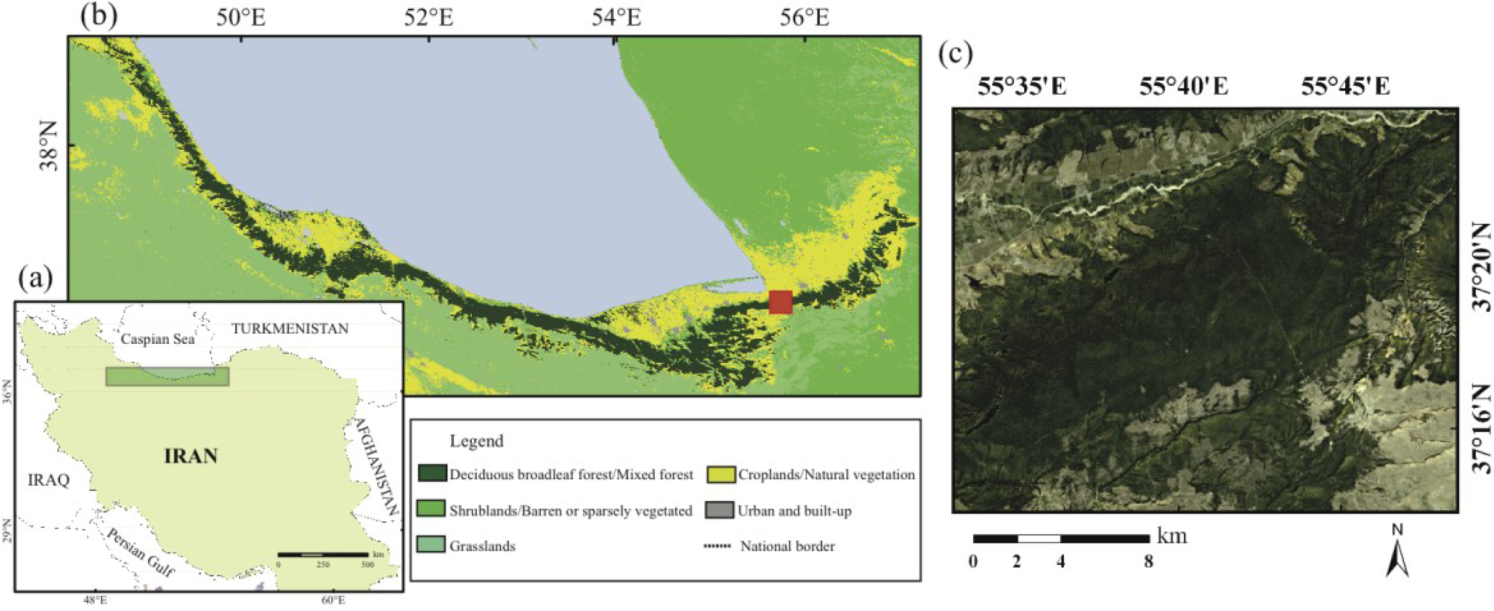
The study area is a subset of the Hyrcanian forest, locally known as the Loveh forest. The Hyrcanian forest stretches over the northern slopes of the Alborz mountains and the southern coast of the Caspian sea. The natural vegetation is temperate deciduous broadleaved forest [26,27].

The Loveh area is located in northern Iran (37°14′ to 37°24′N; 55°33′ to 55°47′E) and comprises ca. 10,683 ha (Figure 1). The elevation ranges from 190 to 1900 m above mean sea level. Slope varies between 6° and 16° on shuttle radar topography mission (SRTM) and a full variety of terrain aspects is observed. Annual mean temperature is 12.2 °C, and annual mean precipitation is 524 mm [23]. Quercus castaneafolia, Carpinus betulus, Acer cappadocicum and Acer velutinum, are the main species. Cerasus avium, Tilia begonifolia, Diospyros lotus, Parrotia persica and Fraxinus excelsior are other available species in the Loveh region [23,25].

The Loveh forest has been treated by shelter-wood method since 1963. The treatment method was replaced with selective logging method in 2003. As a result, tree densities, species richness and the vertical structure of the forest have been modified. Three different stand age classes are found, due to these logging activities [23,24] (

Table 1. Characteristics of main land use classes.

Land Cover Classes	Description
Natural forest * (NF)	The forest has not been affected by any treatment. Trees have closed crown cover. This forest has more developed vertical stratification, and fewer trees per hectare compared to managed stands. It is also composed of trees with larger DBH
Managed forest 1 * (MF1) (5–25 years)	This is the forest area, which is managed by shelter-wood method. Preparatory cut, seed cut and establishment cut were done according to 25 years’ time plan. The removal cut still is not done so some trees with large DBH can be found.
Managed forest 2 * (MF2) (25–45 years)	This forest area is also managed by shelter-wood method for 45 years. Preparatory cut, seed cut as well as establishment and removal cut were done. In average, density of trees (number per hectare) is higher, and trees’ DBH are smaller compared to other classes.
Agriculture land (AG)	Agricultural land refers to agricultural areas purposely provided with water.
Flooded river (FA)	Channel of stream plus any adjacent floodplain areas.

Note:^*[23].

). Preparatory and establishment cuts provided more light for new seedlings to grow in managed stands, however some of the light-dependent species such as Tilia begonifolia, Acer cappadocicum, Diospyros lotus and Parrotia persica were more established than dominant species [28]. Therefore, tree densities increase in managed forest compared to natural forest. The maximum tree density belongs to the MF2, where the long treatment time allows for more seedlings to be established. Because of the existence of some mature trees in MF1 class, the tree diameter at breast height (DBH) and basal area values are higher than MF2 class. However, the largest DBH, basal area and above-ground biomass (AGB) values are observed in natural forest [23]. In this area, agricultural lands and flooded river (adjacent floodplain areas remained from successive floods in 2001, 2002 and 2003 [29]) are also observed and have representative spatial distribution in the study area.

3. Data and Methods

3.1. Field and Remote Sensing Data

Field survey was performed in the summer of 2004 in 99 plots (60 × 60 m) selected by systhematic sampling method. The sample plots were equally distributed among three forest stand age classes in order to be representative of forest over the study area [24]. The geographic center of each sample plot was registered by handheld GPS. Within each plot, DBH were measured and number of trees and tree species were recorded (trees with a DBH ≥ 7.5 cm were included). The field measurements were only used for the description of the forest (

Table 2. Summary of the field plot measurements. Average values per plot are indicated. Standard deviation values are indicated inside parentheses.

Forest Stand Age	DBH (cm)	Trees·ha−1	AGB * (Mg/ha)		Number of Plots
Natural forest (NF)	29.88 (3.6)	306.22 (60.8)		254.27 (29.9)	34
Managed forest 1 (MF1)	21.40 (3.1)	414.46 (53.0)		195.93 (44.7)	32
Managed forest 2 (MF2)	16.90 (3.9)	789.69 (158)		142.14 (32.7)	33

Notes:

^*AGB was calculated from DBH data where AGB = a (DBH)^b : a = 0.0566, b =2.663 [30]. AGB: the total above ground tree dry biomass (Kg/tree); DBH (cm). We calculated the AGB of each tree in the plot. Then we summed up all the values and converted them to Mg/ha.

).

A Landsat-7/ETM+ scene acquired on 10 September 2007 was considered as reference in this investigation. Six reflective bands consisting of visible and short-wave infrared wavelengths with 30 m spatial resolution were used. Thermal and panchromatic bands were not included in this investigation.

ALOS/PALSAR were acquired on 27 September 2007 in fine beam double mode (FBD); HH- and HV-polarization. The scene was delivered in slant range single look complex (SLC) format (level 1.1). We focus on SAR data availability; therefore, there is unavoidable three years’ time shift between field data and remote sensing data. Given our knowledge of forest growth in this area, the delay between remote sensing data acquisition and field survey will not significantly affect classification results. We also use SRTM data (90 m) from US Geological Survey (USGS). We then resample the DEM to 30 m resolution using the cubic convolution interpolation for further procedures described below.

3.2. Methods

3.2.1. Image Processing

Landsat-7/ETM+

The Landsat-7/ETM+ scene was corrected for the scan line corrector (SLC) error using one successive scene (i.e., acquired on 12 October 2007). The scene was then converted to at sensor radiance from digital number (DN), considering the gain and bias of the sensor. In the next step, at sensor radiance was converted to surface reflectance using atmospheric/topographic correction (ATCOR) for sattelite imagary in rugged terrain (ATCOR-3) [31] and SRTM. Atmospheric definition area set to rural in mid-latitude summer. Visibility and adjacency set to 20 and one kilometer, respectively. In order to verify the impact of shadow and relief on the surface reflectance, ETM+ was also atmospherically corrected with identical parameters values based on the ATCOR-2 [31]. We then calculated different vegetation indices [32–38] (

Table 3. Vegetation indices and GLCM textures.

Parameters	Equation	Reference
Vegetation indices
NDVI	(NIR − Red)/(NIR + Red)	[32]
SR	NIR/Red	[33]
SAVI	[1.5(NIR − Red)]/[NIR + Red + 0.5]	[34]
SARVI	[2.5(NIR − Red)]/[1 + NIR + (6 × Red) − (7.5 × Blue)]	[35]
SLAVI	NIR/(Red + MIR2)	[36]
Infrared index	(NIR − MIR1)/(NIR + MIR1)	[37,38]
Textures		[42]
Mean	${\mu }_i=\sum _{i,j=0}^{N-1}i{\left(p_{i,j}\right)}^{*}$
Variance	${\sigma }_i^2=\sum _{i,j=0}^{N-1}{p}_{i,j}{}^{*}{\left(i-{\mu }_i\right)}^2$
Contrast	$\sum _{i,j=0}^{N-1}{p}_{i,j}{}^{*}{\left(i-j\right)}^2$
Correlation	$\sum _{i,j=0}^{N-1}{p}_{i,j}{}^{*}\left[\left(i-{\mu }_i\right)\left(j-{\mu }_j\right)/\sqrt{\left({\sigma }_i^2\right)\left({\sigma }_j^2\right)}\right]$
Dissimilarity	$\sum _{i,j=0}^{N-1}{p}_{i,j}{}^{*}|i-j|$
Entropy	$\sum _{i,j=0}^{N-1}{p}_{i,j}{}^{*}\left(-\text{ln}{p}_{i,j}\right)$
Second moment	$\sum _{i,j=0}^{N-1}{p}_{i,j}{}^{2*}$
Homogeneity	$\sum _{i,j=0}^{N-1}{p}_{i,j}{}^{*}/1+{\left(i-j\right)}^2$

Notes: NDVI, normalized difference vegetation index; SR, simple ratio; SAVI, soil adjusted vegetation index; SARVI, soil and atmosphere resistant vegetation index; SLAVI, specific leaf area vegetation index. Blue: band 1 ETM+, ρ = 485 nm; red: band 3 ETM+, ρ = 660 nm; near infrared (NIR): band 4 ETM+, ρ = 835 nm; middle infrared 1 (MIR1): band 5 ETM+, ρ = 1650 nm; middle infrared 2 (MIR 2): band 7 ETM+, ρ = 2220 nm. The wavelengths indicate the center of the Landsat spectral bands.

^*$p_{i,j}=v_{i,j}/{\sum }_{i,j=0}^{N=1}{v}_{i,j}$, where v_i,j is the value in the cell i,j (row i and column j) of the moving window and N is the number of rows or columns.

), principal component analysis (PCA) [39], tasseled cap transformation (TCT) [40,41] and gray level co-occurrence matrix (GLCM) [42] from the topographic compensated surface reflectance (Table 3). Vegetation indices, PCA, TCT and GLCM textures of optical data are widely used for retrieval of the forest structure as well as land cover and forest stand age classification [24,43–45]. Window size affects the role of GLCM textures in land cover classification [46,47]. Small window sizes often exaggerate differences and increase the noise content on the texture image, while large window sizes cannot effectively extract the texture information due to smoothing texture variation [46–49]. Based on visual interpretation and the separabilities among land cover classes, we chose the window size of 11 × 11 pixels with horizontal and vertical offset of one.

ALOS/PALSAR

In order to enhance radiometric resolution and to square the pixels in ground range geometry at similar spatial resolution (i.e., 30 m for Landsat), the amplitude images were multi-looked eight times for the dual-polarization scene (i.e., four looks in azimuth and two looks in range) [50,51]. We then performed refined Lee filter by a window size of 7 × 7 in order to minimize speckle noise [52]. The performance of the filter and selection of the optimal window size were evaluated with the speckle suppression and mean preservation index (SMPI; [53]).

The intensity scenes were converted into their corresponding radar backscattering coefficients (Sigma nought, dB; σ^°) values (Equation (1)) [54,55].

$${\sigma }^{\circ }=10\times {\text{log}}_{10}\left({\text{I}}^2+{\text{Q}}^2\right)+\text{CF}-32.0$$

(1)

CF (calibration factor) = −83 dB, I and Q are the real and imaginary parts of the complex SAR image pixel value.

Since the study area is mountainous and a strong relief effect is observed, we performed radiometric terrain correction to compensate for the ground-topography influence on radar backscattering coefficient. The corrected backscatter in gamma-nought γ^° format can be obtained from the sigma-nought σ^° value according to Equation (2) [56,57].

$${\gamma }^{\circ }={\sigma }^{\circ }\frac{{\text{A}}_{\text{flat}}}{{\text{A}}_{\text{slope}}}{\left(\frac{\text{cos}{\theta }_{\text{ref}}}{\text{cos}{\theta }_{\text{loc}}}\right)}^{\text{n}}$$

(2)

where γ^° is topographic normalized radar backscattering coefficient, σ^° is radar backscattering coefficient, A_flat is PALSAR pixel size for a theoretical flat terrain, A_slope is true local PALSAR pixel size for the mountain terrain, θ_loc is local incidence angle and θ_ref is radar incidence angle at the image center.

The exponent n is the optical canopy depth and ranges between 0 and 1. It is a site-specific factor and difficult to obtain in practice, therefor it is set to 1 [58–61].

We calculated alpha angle (α), entropy (H) and anisotropy (A) (

Table 4. Alpha—Entropy decomposition parameters.

Parameters	Equation	Reference
Alpha	${\sum }_{i=1}^3{P}_i*{\alpha }_i$	[62]
Entropy	${\sum }_{i=1}^3-P_i{\text{log}}_3{P}_i$
Anisotropy	λ2** − λ3** / λ2** + λ3**

Note:^*$p_i={\lambda }_i/{\sum }_{j=1}^3{\lambda }_j$,^**λ_j: eigen values from coherency matrix [62].

) according to Alpha-Entropy decomposition proposed by Cloude and Pottier [62]. Cloude and Pottier have proposed a method of the extraction of mean diffusion based on eigenvalues/eigenvectors decomposition of the coherence matrix in order to characterize scattering interactions of the beams with the targets [62]. High values of alpha stand for volume or multiple scattering mechanisms and low values associate with surface scattering [62]. Entropy indicates the randomness or statistical disorder of the target [62]. We also used GLCM (Table 3) in order to extract textural features from both HH and HV polarization channels. GLCM textures show to be useful to discriminate different forest regeneration stages [7,63]. As mentioned in Section “Landsat-7/ETM+”, selecting the appropriate window size for texture analysis is important. We choose the window size of 11 × 11 with horizontal and vertical offset of one based on the visual interpretation and the separabilities among land cover classes on texture layers.

3.2.2. Determination of the Land Cover Classification Scheme

In order to select homogeneous regions of each land use class (Table 1), we made use of the in situ measurements and previous land use/land cover map of the area [64]. We also used 15 historical Landsat scenes, which encompass the period from 1986 to 2007. We performed unsupervised classification and visual interpretation of these scenes to ensure the forest boundaries, map different forest stand age classes over time and cross-check the previous land use/land cover map. The in situ measurements were useful for delineating the current status of different stand age classes of forest. Approximately 300 pixels of each land cover class were selected to represent land cover types over the study area. We used 70% of each class (ca. 200 pixels) for training and 30% (ca. 100 pixels) for validation purposes. Separability analyses were performed based on the transformed divergence (TD) index. TD is a measure of separability between a pair of classes [65,66]. The divergences values can range from 0 to 2 and indicate how well the selected pairs of classes are statistically separable from each other. Higher values indicate better separation [65,67].

We divided the datasets into three major groups, (A) surface reflectance bands from Landsat-7/ETM+ scene; and pertinent features; (B) individual ALOS/PALSAR intensity backscattering and derived features and (C) the combination of both Landsat-7/ETM+ and ALOS/PALSAR data. The group B is divided into five subgroups (e.g., B1–B5) whose details are given in

Table 5. Proposed scenarios for the classification scheme.

Group	Subgroup	Datasets	Selected features
A		ETM+ spectral bands, GLCM, vegetation indices, PCA, TCT	ETM+ spectral bands, pca-1 *, wet *, br *, con * b1, con * b2, cor * b3, me * b4, var * b4, cor * b4, cor * b5, me * b6, SLAVI
B	B1	SAR bands	HH, HV
	B2	SAR bands, GLCM textures of HV	HH, HV, hom * HV, dis * HV
	B3	SAR bands, GLCM textures of HH	HH, HV, ent * HH, sm * HH
	B4	SAR bands, polarimetric features	HH, HV, alpha, entropy
	B5	SAR bands, polarimetric features, textures of HH, HV	HH, HV, alpha, entropy, hom * HV, dis * HV, ent * HH and sm * HH
C		ETM+ data and SAR data	ETM+ spectral bands, pca-1 *, wet *, br *, con * b1, cor * b3, me * b4, cor * b4, cor * b5, SLAVI HH, HV, alpha, entropy, hom * HV, dis * HV, ent * HH and sm * HH

Notes:

^*pca-1: first component of PCA; br: brightness; wet: wetness; con: contrast; cor: correlation; me: mean; hom: homogeneity; dis: dissimilarity; ent: GLCM entropy; sm: second moment.

.

In order to maximize the classification accuracy, it is necessary to identify the best combination of textural bands as well as indices and features. In fact, not all the derived features are informative for land cover classification, or some of them may contain similar information [68]. We initially selected the texture bands with high separability. Then, we checked the correlation among different textural bands to reduce the data redundancy [40,68]. The final selection of pertinent features was based on experimental classification results. We fallowed the same procedure for selecting among vegetation indices and other features.

Because of the different nature of the data proposed in the classification scheme (Table 5), we evaluated three different non-parametric classifiers: support vector machines (SVM), neural network (NN) and random forest (RF). We also performed maximum likelihood classification (MLC) in order to compare its performance with non-parametric classifiers. MLC is a parametric classifier that assumes normal or near normal distribution for each feature of interest [68]. Despite limitations due to its assumption of normal distribution of class signature [69], it is perhaps one of the most widely used classifiers [70–72]. Non-parametric approaches are suggested for the classification of multi-source data in complex environments [73]. SVM is a supervised non-parametric statistical learning technique [74] and it follows what is known as structural risk minimization. SVM is particularly appealing in remote sensing due to its ability to handle small training datasets successfully [75–78]. SVM minimizes classification error on unseen data without prior knowledge about the probability distribution of the data [75–77]. It creates a hyperplane through n dimensional spectral-space that separates classes based on a user defined kernel function and parameters such as penalty parameter. These parameters are optimized using machine learning to maximize the margin from the closet point to the hyperplane. A penalty parameter allows the SVM to vary the degree of training data misclassified due to possible data error when optimizing the hyperplane [79]. Linear, polynominal, radial basis function and sigmoid are the four common kernels available in remote sensing packages. A careful selection of parameter setting can improve the performance of the SVM [80].We applied SVM with the radial basis function and penalty parameter of 100, which is also shown by Yang [80], as the best kernel and parameter for land cover classification [79]. NN is also a nonparametric classifier with arbitrary decision boundary capabilities, easy adaptation to different data types and input structures as well as fuzzy output values and good generalization for use with multiple images [81]. It benefits from parallel computation, the ability to estimate the non-linear relationship between the input data and desired outputs, and fast generalization capability [82,83]. The parameter setting was based on experimental results. The logistic function as an activation function, one hidden layer and 1000 training iterations were selected. RF is a machine ensemble approach that makes use of multiple self-learning decision trees to parameterize models and use them for estimating categorical or continuous variables [84,85]. RF can be used to learn complex non-linear relationships, such as those presented in variable vertical structure. Therefore, it is very efficient for classify complex and heterogeneous landscape [85]. The number of variables is a user-defined parameter, as we had selected the layers in each dataset; therefore, we used all selected layers. Non-parametric classifiers often produce higher classification accuracy than the traditional parametric classifiers [75–77,81,82,84,85].

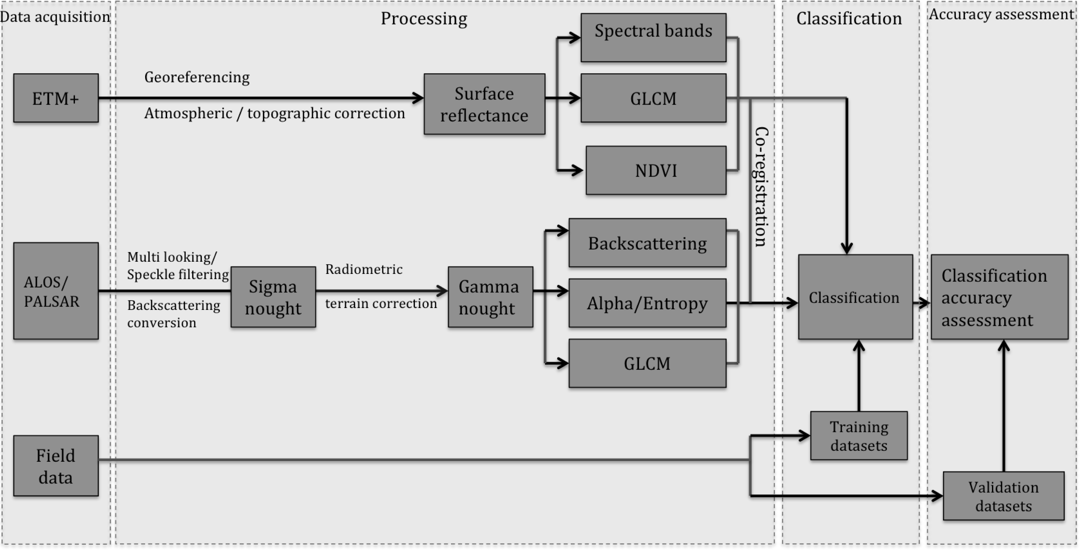
We then calculated producer’s accuracy (PA), user’s accuracy (UA) and overall accuracy (OA) from the classification results. Producer’s accuracy measures the omission error to a certain class and it is the probability of a reference site being correctly classified. User’s accuracy is the measure of commission error or the probability that a pixel classified on the image actually represents that class on the ground [86]. The overall accuracy is the percentage of the correctly classified pixels in the validation dataset [86]. We used Z-test to evaluate statistical significance differences in classification accuracy statistics [87]. Figure 2 provides an overview of the entire approach adopted in this investigation.

4. Results

4.1. Spectral, Backscattering and Polarimetric Characterization

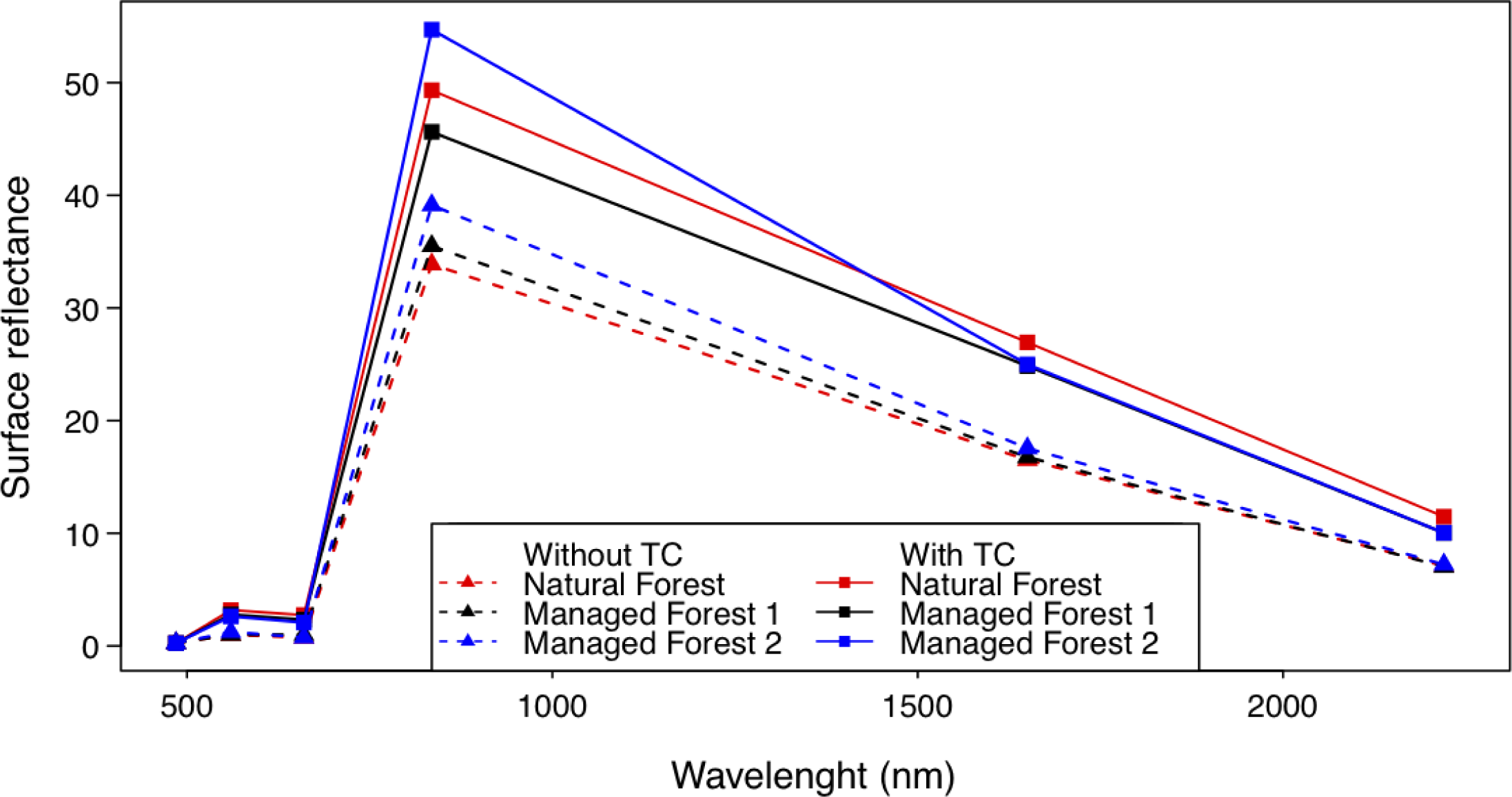
Landsat surface reflectances for training dataset without and with topographic correction are shown in Figure 3. The topographic effects tend to decrease the surface reflectance in green, NIR and shortwave infrared (SWIR) regions due to the shadowing effects introduced by the relief and orientation of faced region (Figures 3).

After terrain correction, MF2 has the highest reflectance at NIR and the lowest reflectance at red. This particular forest class, subjected to intensive logging treatments, shows only one well-structured canopy layer, and less shadow effects among canopies. On the other hand, less intervention by logging at MF1 tends to preserve the vertical structure of the forest making the discrimination between NF and MF1 a challenging task [24]. Different forest stand age classes may present similar canopy structure even with different ages, species complexity and biomass amounts; therefore, it is difficult to classify them based on surface reflectance [19]. However, the spectral behavior and separability are in agreement with previous investigation in this study area using Landsat ETM+ data [24].

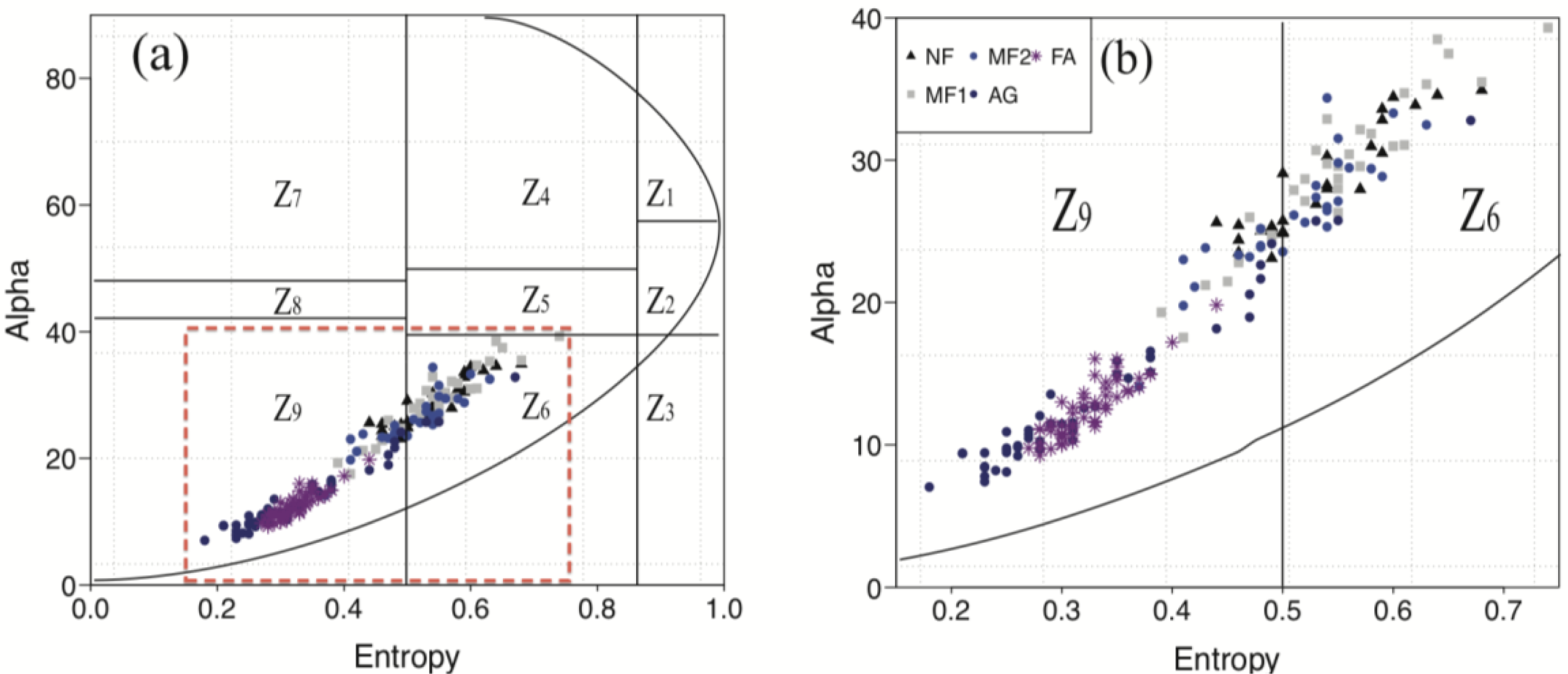
Figure 4 shows training datasets plotted on the Alpha-Entropy segmentation plane. Different forest stand age classes overlap each other showing predominantly surface scattering with moderate alpha values and relative high entropy values in dual polarization mode. The range of alpha and entropy values for different stand age classes in dual polarimetric mode is not wide enough to separate different classes. Agricultural land and flooded river represent surface scattering with relatively low alpha and entropy values.

Table 6. Average values of the intensity backscattering at HH, HV, alpha and entropy for different land cover classes. The results are based on the training dataset. See Table 1 for the descriptions of classes.

Land Cover Classes	HH Backscattering (dB)	HV Backscattering (dB)	Alpha (°)	Entropy
NF	−8.56	−12.72	26.66	0.82
MF1	−9.12	−13.24	28.25	0.85
MF2	−9.75	−13.48	28.82	0.86
AG	−15.24	−23.89	13.35	0.53
FA	−12.79	−21.32	12.54	0.52

presents average values of the intensity backscattering at HH, HV as well as alpha and entropy for each land cover class. The backscattering values in both HH and HV polarized bands (Table 6) tend to decrease from NF to the both managed forest classes due to a more clear forest floor. Less density of trees per ha might enhance forest scattering (Table 6). Comparing the backscattering values in co-polarized band (HH) and cross-polarized band (HV) shows that all forest classes have higher backscattering in HH polarized band. This occurs because of the higher sensitivity of HH to volume scattering, which is influenced by the random distribution of branches, twigs and leaves [7]. The use of dual-polarization data rather than quad-polarization—which was not available for the study area—could also affect the results [7]. Forest classes show higher alpha values compared to other classes (Table 6).

4.2. Assessment of the Spectral Separability

Table 7. Transformed divergence (TD) index for different forest class pairs, TD values higher than the threshold (TD ≥ 1.8) are in bold.

Groups	Class Pairs
	Natural Forest–Managed Forest 1	Natural Forest–Managed Forest 2	Managed Forest 1–Managed Forest 2
A	1.85	1.9	1.9
B1	0.05	0.34	0.19
B2	0.92	1.21	0.49
B3	0.69	1.11	0.56
B4	0.22	0.76	0.56
B5	1.67	1.83	1.45
C	2	2	2

compares the separability index for different combinations of forest class pairs. Groups A and C have high separability indices, showing a good separation between forest classes. In group B, except in subgroup B5, the separability indices between forest classes are low, showing that different forest stand age classes are difficult to separate with dual polarimetric SAR. Including SAR textures and derived features as well as polSAR bands (subgroup B5) significantly enhance the separability index (TD ranges from 1.45 to 1.83).

In all datasets, the separability index for pair “NF-MF2” are greater than “NF-MF1”. That could be the effect of long term treatment on managed stand during 45 years (MF2), which leads to different forest structure to natural forest [23,24]. In most datasets, separability index of “MF1-MF2” is the lowest, which makes the separation between two managed forest classes difficult.

4.3. Effect of Terrain Correction on Classification Accuracies

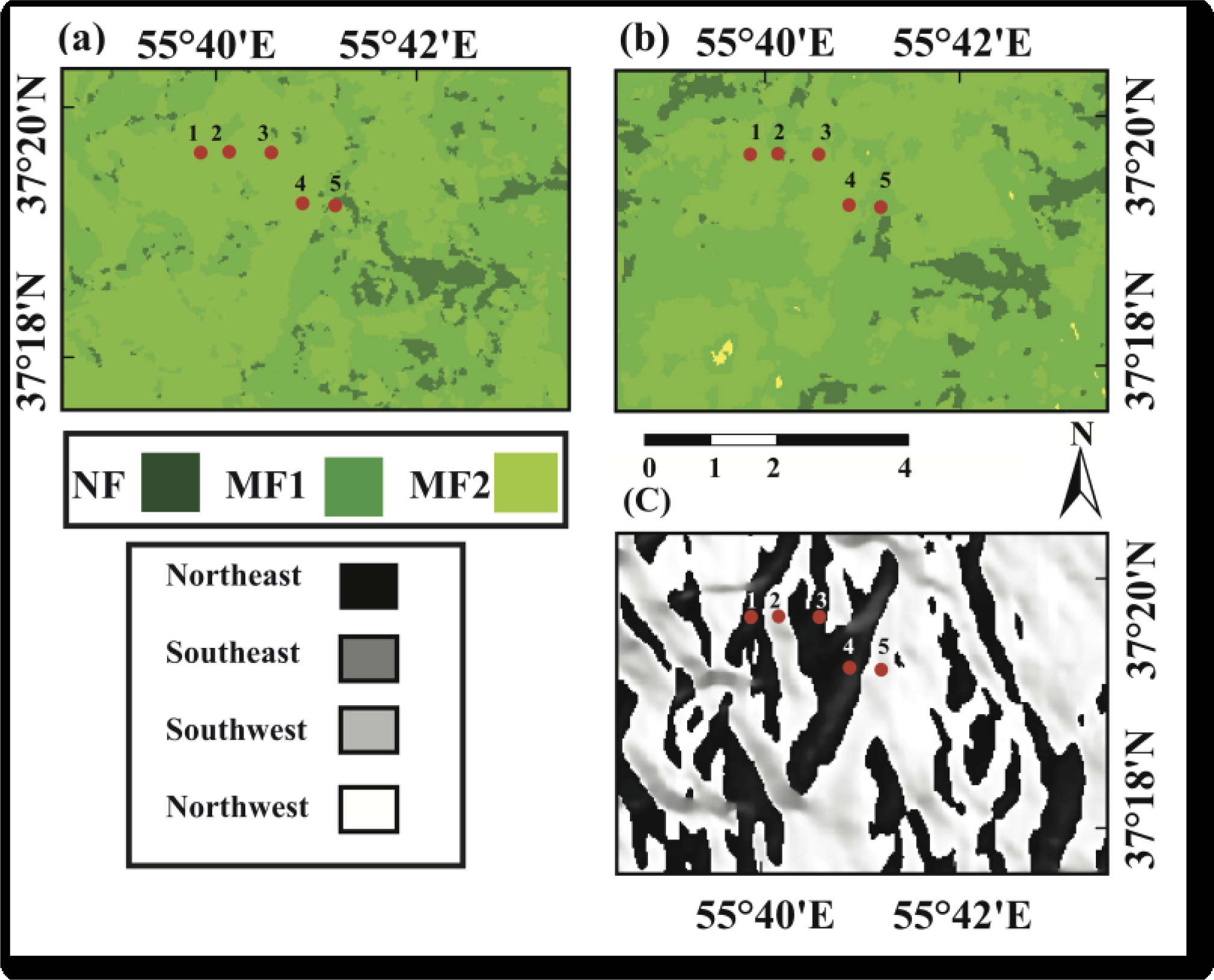
In order to show the effect of topography on classification results, we classified the dataset C with non-topographically corrected ETM+ data. Figure 5 highlights the effect of different facing slopes on classification results. A subset of classification results (Figure 5a) with, and (Figure 5b) without topographic effects, and (Figure 5c) aspect map are displayed. Points 1, 2 and 3 belong to MF2 class, located on different facing slopes. In Figure 5a, they are classified correctly. In Figure 5b, point 2 is misclassified as class MF1 because of presence of illumination effect. The same effect is observed for points 4 and 5. Both belong to MF2 class. In Figure 5b, point 5 is wrongly labeled as MF1.

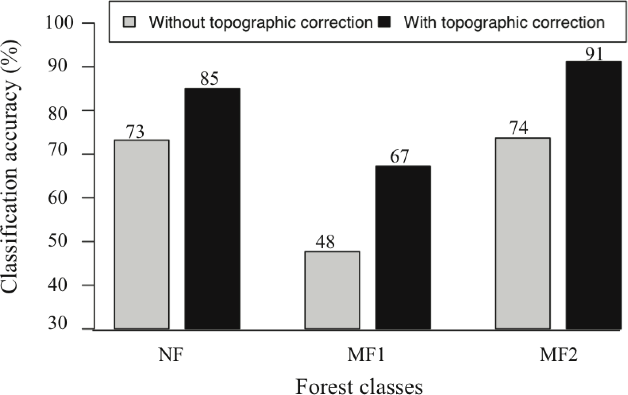
The average classification accuracy of non-topographically corrected ETM+ is 65% (from non-parametric classifiers). Figure 6 illustrates the SVM classification accuracies without and with topographic correction for three forest classes for datasets C. Our results demonstrate that high relief in the mountainous area reduces the classification accuracy. The same trend is reported by others [22,88]; we therefore focused on classification of terrain corrected datasets.

4.4. Performance Comparison of MLC, SVM, RF and NN Classifier

In

Table 8. Classification overall accuracy of datasets. See Table 5 for the descriptions of groups.

Groups	Classifier
	MLC	SVM	NN	RF
A	84.81 a	84.92 a	85.57 a	84.21 a
B1	48	61.28 b	53.43	62 b
B2	57.71	71.07	56.64	82.71
B3	57.73	71 c	70.57 c	79
B4	62.8	75.64 d	71.64	77.93 d
B5	70.42	80 e	74.05	81.93 e
C	82.1	86.35 f	83.9	85.57 f

Note: The identical superscripts show that the differences between the comparison cases are not statistically significant (5% significance level).

, the classification results of four classifiers in each group are presented. The performances of four classifiers within each group are compared at 5% significance level.

Table 9. User/producer accuracy. See Tables 1 and 5 for the descriptions of land cover classes and groups.

		User Accuracy							Producer Accuracy
MLC		Land Cover Classes							Land Cover Classes
		NF	MF1	MF2	AG	FA			NF	MF1	MF2	AG	FA
Groups	A	74.84	70.37	79.59	99.03	100.00	Groups	A	76.04	72.61	79.12	95.64	99.37
	B1	35.74	29.62	38.51	55.85	88.45		B1	33.23	32.17	36.47	65.42	76.80
	B2	51.04	40.13	47.38	57.55	91.36		B2	46.96	39.49	45.29	68.85	86.21
	B3	49.18	44.62	49.84	59.18	86.01		B3	47.92	46.18	46.76	67.29	79.00
	B4	53.75	42.47	64.55	64.79	88.85		B4	52.72	44.90	56.76	71.65	87.46
	B5	73.87	58.49	68.95	66.94	90.21		B5	67.73	59.24	62.06	76.95	92.48
	C	66.98	68.36	76.61	96.90	99.37		C	68.69	55.73	87.65	97.51	99.06
SVM		Land cover classes							Land cover classes
		NF	MF1	MF2	AG	FA			NF	MF1	MF2	AG	FA
Groups	A	75.68	74.16	80.64	99.05	100.00	Groups	A	79.55	70.38	82.06	97.82	99.37
	B1	61.28	49.26	55.42	65.97	77.14		B1	58.15	52.87	52.65	68.85	76.18
	B2	67.11	57.01	68.09	70.03	91.32		B2	64.54	57.01	60.88	82.24	89.03
	B3	67.56	58.75	70.66	66.57	91.91		B3	64.54	59.87	65.88	75.08	89.03
	B4	64.71	55.91	70.55	86.17	99.33		B4	63.06	61.78	64.12	93.15	93.10
	B5	78.48	65.94	77.95	86.25	96.50		B5	75.72	67.20	73.82	93.77	94.98
	C	78.40	81.96	80.79	94.36	96.74		C	84.66	66.56	90.29	93.77	94.98
NN		Land cover classes							Land cover classes
		NF	MF1	MF2	AG	FA			NF	MF1	MF2	AG	FA
Groups	A	73.45	70.03	77.68	99.06	100.00	Groups	A	79.55	66.24	76.76	98.13	99.37
	B1	43.01	35.80	42.17	55.73	88.32		B1	39.30	36.94	38.82	68.22	80.56
	B2	53.96	42.55	46.04	56.74	91.26		B2	47.92	43.63	44.41	69.47	81.82
	B3	65.58	56.31	68.25	70.67	92.72		B3	64.54	52.55	63.24	82.55	91.85
	B4	62.68	52.24	70.85	72.85	95.13		B4	56.87	55.73	66.47	81.93	91.85
	B5	64.08	53.50	67.91	85.43	99.33		B5	63.06	56.05	64.12	93.15	93.10
	C	69.54	72.22	76.61	97.21	99.69		C	72.20	57.96	87.65	97.82	99.37
RF		Land cover classes							Land cover classes
		NF	MF1	MF2	AG	FA			NF	MF1	MF2	AG	FA
Groups	A	70.94	72.48	79.34	99.06	100.00	Groups	A	79.55	59.55	84.71	98.13	99.37
	B1	58.82	43.58	54.37	67.45	90.70		B1	47.92	49.68	49.41	80.69	85.58
	B2	78.55	67.21	77.95	86.83	99.35		B2	79.55	65.29	73.82	96.57	95.30
	B3	70.54	64.03	74.21	85.19	99.33		B3	75.72	61.78	69.41	93.15	93.10
	B4	68.91	59.69	72.17	86.92	99.33		B4	68.69	61.78	69.41	93.15	93.10
	B5	78.55	67.21	77.95	86.25	96.50		B5	79.55	65.29	73.82	93.77	94.98
	C	72.31	73.49	77.95	99.37	100.00		C	75.08	59.80	89.41	98.13	99.69

presents the user and producer accuracy for each class. All classifiers show balanced PA and UA, as the differences between user and producer accuracies are not high [89]. The results of classification of Landsat and its derived features show that MLC as well as the three machine learning classifiers have good performance (average OA = 84%) and there is no statistically significant difference (at 5% significance level) in their results. In group B, MLC has poorer performance compared to non-parametric classifier. In this group, except for those datasets that SAR textures (B2 and B3) are used, SVM and RF have the same performance and there is no substantial difference in their performances at 95% confidence level. Also, in all datasets SVM and RF produce better classification value at 95% confidence level compared to NN. B3 is the only dataset that NN and SVM have the similar results. In group C, MLC provides the poorest accuracy compared to non-parametric classifiers. In this group, SVM and RF have better performance at 5% significance level. Based on the relatively poor performance of MLC compared to non-parametric classifiers for ALOS/PALSAR classification, it was not considered in further analysis.

4.5. Assessment of the Classification Accuracy of ALOS/PALSAR

Here, we evaluated the contribution of polarimetric features and textures of polarized bands in classification overall accuracy at the 95% confidence level (

Table 10. Z-test ^* results for the comparison of overall accuracies of B1 versus B2–B5. See Table 5 for the descriptions of subgroups.

	Classifier
	SVM	NN	RF
B1 versus B2	6.91	4.84	13.57
B1 versus B3	7.31	11.72	10.48
B1 versus B4	10.91	12.23	10.29
B1 versus B5	14.1	14.27	13.03

Notes:

^*Absolute Z value at the 5% significance level is equal to 1.96. The comparison cases with Z value greater than absolute Z value are statistically different at 95% significance level.

). For each classifier, we performed Z-test between classification results of B1 and other datasets in group B. Absolute Z value at the 5% significance level is equal to 1.96. The comparison cases with Z value greater than absolute Z value are statistically different at 95% significance level. Table 10 summarizes the results of Z-test in group B. In subgroup B1, we classified HH and HV PolSAR bands. We added textures of HV to subgroup B2 and textures of HH to subgroup B3. We classified alpha, entropy and anisotropy as well as HH and HV polarimetric bands in subgroup B4. In Subgroup B5, PolSAR and their derived features are entered into classification algorithms. B1 has the lowest overall accuracy (average OA = 59%; Table 8). Considering UA and PA of each class, the order from highest to lowest is FA, AG, NF, MF2, and MF1 (Table 9). In B2 and B3, the average overall accuracies reach 70% and 73%, respectively (Table 8). The comparison among individual item classification show higher accuracies in subgroup B3 compared to B2 (Table 9). This could be explained by higher sensitivity of HH polarization to volume scattering. In B4, the average overall accuracy increases significantly to 75% (Table 8). The PA and UA values, especially in forest classes, significantly increase compared to B1, B2 and B3 (Table 9). In B5, we obtained the best classification results based on SAR data (average OA = 78%; Table 8). Regardless of the classifier, we concluded that HH and HV cannot separate different forest stand age classes properly, however textures of HH, HV as well as polarimetric features significantly (at 95% confidence level) increase the classification overall accuracies.

4.6. Classification of ETM+ and ALOS/PALSAR

Table 8 summarizes classification results of four classifiers for each dataset. We performed Z-test at 95% significance level between the classification results of group A versus each dataset to investigate the effect of different datasets on classification accuracy. We did the comparison among the results of each classifier separately in order to exclude the effect of classifier’s performance. In group A, accuracies of classes AG and FA are higher compared to forest classes in all classifiers. Among forest classes, MF2 has the highest PA and UA values and MF1 in most cases has the lowest accuracies. Classification of Landsat spectral bands and its derived features (group A) produces high overall accuracy values with all classification algorithms (average OA = 85%; Table 8). Classification results of ETM+ indicate that medium resolution spectral bands of ETM+ data can classify the land cover efficiently.

In group B, FA has the highest PA and UA values. Forest classes do not follow the same trend in different subgroups. In most cases, the order of forest classes from highest to lowest PA and UA is NF, MF2 and MF1. The overall classification values vary substantially depending on input data. HH and HV cannot separate different forest stand age classes (average OA = 59%) properly. However, alpha, entropy and anisotropy as well as GLCM textures increase the average overall accuracy to 78%. Although, this overall accuracy does not overcome the overall accuracy from ETM+ dataset (OA = 84%) at 95% confidence level; however, it shows that in the absence of optical data (e.g., Landsat ETM+), SAR data can be used alternatively for classification purposes. This result is also in accordance with previous studies [3,7]. In the last dataset, C, both Landsat-7/ETM+ and SAR data are jointly classified. Considering UA and PA of each class, the order from highest to lowest is FA, AG, MF2, NF and MF1 (Table 9). The classification accuracies of dataset C (OA = 86%) are significantly (at 95% confidence interval) different from datasets A and B. However, the joint process of ETM+ and ALOS/PALSAR does not greatly improve the classification overall accuracy, and it is very close to the original ETM+ classification.

5. Discussion

In this study, Landsat and ALOS/PALSAR data have been classified—separately and jointly—for mapping complex mountainous forests. Good classification results from medium resolution spectral bands of ETM+ data show its high applicability in mapping heterogeneous forest. The ETM+ classification result is inconsistent with results from previous investigation conducted in this study area [24]. Forest stand age classification results based on backscattering at HH and HV are not satisfactory. Different forest classes have similar backscattering at HH and HV, which makes the separation among different classes a challenging task. The saturation effect in backscattering values, which occurs in such high biomass forest (i.e., >100 Mg/ha), may cause backscattering similarity in dual polarized bands [7,90,91]. Separability values among forest classes increase by adding textures and polarimetric features. The acceptable separability is only observed when all polSAR features are used. The classification result of this dataset is satisfactory; however, it does not overcome Landsat classification result. It indicates that in the absence of optical data (e.g., Landsat ETM+), SAR data can be used alternatively for classification purposes. This result is also in accordance with previous studies [3,7]. Integration of Landsat and ALOS/PALSAR slightly increases the classification accuracy. However, the improvement is not substantial and the result is very close to the original Landsat classification. The structure similarity in different forest classes in dual polarimetric SAR could be one probable reason for this result.

A comparison among the performances of both parametric and non-parametric classifiers showed that all classifiers have good performance for Landsat classification. MLC cannot effectively classify SAR data. It is probably because of its assumption of features’ normal or near normal distribution, which may not be the case for forest SAR backscattering. In almost all SAR datasets, SVM and RF produce better classification values at 95% confidence level compared to NN. Classifiers have the same performance for classification of the joint dataset; SVM and RF have better performance compared to NN and MLC at 5% significance level. Parametric classification algorithms such as MLC are not typically suitable for multi source data [73,84]. The better performance of SVM and RF compared to NN could be because of the fact that both of these classifiers can handle high dimensional data [77,84].

6. Recommendations and Conclusions

High classification accuracy achieved by inclusion of SAR textures and PolSAR decompositions shows that in the absence of optical data (due to the frequent cloud coverage in this region), SAR data can be used alternatively for classification purposes in complex mountainous forest. The joint process of dual polarimetric L-band SAR and ETM+ slightly improves the classification accuracy. The classification results are very close to original ETM+ classification, not only in the overall accuracy, but also in individual item classification accuracy. Our results also confirm that terrain correction is essential prior to data classification in those regions. The outcomes of SVM, NN and RF proved the robustness of nonparametric classifiers at 5% significance level for stand age forest classification in mountainous regions. All classifiers have similar overall accuracy for ETM+ classification. However, SVM and RF are considered more effective for the joint classification of ETM+ and SAR. MLC was as powerful as non-parametric classifiers in ETM+ classification; however, it did not show a good performance in case of SAR data classification. Although, the selection of a suitable classifier depends on tradeoffs among classification accuracy, time consumption, and computing resources.

While these results for the joint application of optical and SAR data for classification purposes in the mountain area are promising, there are several important points that should be taken into account for further investigation. Backscattering similarity in dual polarimetric mode is one of the reasons for relatively low overall accuracy resulting from SAR backscattering. Therefore, it is recommended to investigate the full polarimetric L-band SAR for forest stand age classification purposes. However, the ALOS/PALSAR mission ended in 2011, so currently no spaceborne L-band SAR exists. There are some planned spaceborne L-band SAR missions such as ALOS/PALSAR-2, TanDEM-L, MAPSAR and DESDynI. The prospective spaceborne SAR have some advantages over ALOS/PALSAR, such as more consistent multi-annual coverage as well as shorter repeat intervals for improved interferometric applications [10]. Because of the sensitivity of SAR backscattering to soil and vegetation moisture [7], the prospective research shall focus also on precipitation events prior to capturing the data.

References

- Lefsky, M.; Cohen, W. Selection of Remotely Sensed Data. In Remote Sensing of Forest Environments; Wulder, M., Franklin, S., Eds.; Springer: New York, NY, USA, 2003; pp. 13–46. [Google Scholar]
- Lu, D.; Weng, Q. A survey of image classification methods and techniques for improving classification performance. Int. J. Remote Sens 2007, 28, 823–870. [Google Scholar]
- Lu, D.; Li, G.; Moran, E.; Dutra, L.; Batistella, M. A comparison of multisensor integration methods for land Cover classification in the Brazilian Amazon. GISci. Remote Sens 2011, 48, 345–370. [Google Scholar]
- Vaglio Laurin, G.; Liesenberg, V.; Chen, Q.; Guerriero, L.; del Frate, F.; Bartolini, A.; Coomes, D.; Wilebore, B.; Lindsell, J.; Valentini, R. Optical and SAR sensor synergies for forest and land cover mapping in a tropical site in West Africa. Int. Appl. Earth Obs. Geoinf 2013, 21, 7–16. [Google Scholar]
- Corcoran, J.; Knight, J.; Gallant, A. Influence of multi-source and multi-temporal remotely sensed and ancillary data on the accuracy of random forest classification of wetlands in northern Minnesota. Remote Sens 2013, 5, 3212–3238. [Google Scholar]
- Ghulam, A.; Porton, I.; Freeman, K. Detecting subcanopy invasive plant species in tropical rainforest by integrating optical and microwave (InSAR/PolInSAR) remote sensing data, and a decision tree algorithm. ISPRS J. Photogramm. Remote Sens 2014, 88, 174–192. [Google Scholar]
- Liesenberg, V.; Gloaguen, R. Evaluating SAR polarization modes at L-band for forest classification purposes in Eastern Amazon, Brazil. Int. J. Appl. Earth Obs. Geoinf 2013, 21, 122–135. [Google Scholar]
- Asner, G.P. Cloud cover in Landsat observations of the Brazilian Amazon. Int. J. Remote Sens 2001, 22, 3855–3862. [Google Scholar]
- Leckie, D.; Ranson, K. Forestry applications using imaging radar. Princ. Appl. Imaging Radar 1998, 2, 435–509. [Google Scholar]
- Cartus, O.; Kellndorfer, J.; Rombach, M.; Walker, W. Mapping canopy height and growing stock volume using airborne lidar, ALOS PALSAR and Landsat ETM+. Remote Sens 2012, 4, 3320–3345. [Google Scholar]
- Rosenqvist, A.; Shimada, M.; Ito, N.; Watanabe, M. ALOS PALSAR: A pathfinder mission for global-scale monitoring of the environment. IEEE Trans. Geosci. Remote Sens 2007, 45, 3307–3316. [Google Scholar]
- Clewley, D.; Lucas, R.; Accad, A.; Armston, J.; Bowen, M.; Dwyer, J.; Pollock, S.; Bunting, P.; McAlpine, C.; Eyre, T.; et al. An Approach to mapping forest growth stages in Queensland, Australia through integration of ALOS PALSAR and Landsat sensor data. Remote Sens 2012, 4, 2236–2255. [Google Scholar]
- Lehmann, E.; Caccetta, P.; Zhou, Z.S.; Mitchell, A.; Tapley, I.; Milne, A.; Held, A.; Lowell, K.; McNeill, S. Forest Discrimination Analysis of Combined Landsat and ALOS-PALSAR Data. Proceedings of the International Symposium for Remote Sensing of the Environment, Sydney, Australia, 10–15 April 2011.
- Robinson, C.; Saatchi, S.; Neumann, M.; Gillespie, T. Impacts of spatial variability on aboveground biomass estimation from L-Band radar in a temperate forest. Remote Sens 2013, 5, 1001–1023. [Google Scholar]
- Galvao, L.S.; Ponzoni, F.J.; Liesenberg, V.; Santos, J.R.D. Possibilities of discriminating tropical secondary succession in Amazonia using hyperspectral and multiangular CHRIS/PROBA data. Int. J. Appl. Earth Obs. Geoinf 2009, 11, 8–14. [Google Scholar]
- Shimabukuro, Y.E.; Almeida-Filho, R.; Kuplich, T.M.; de Freitas, R.M. Quantifying optical and SAR image relationships for tropical landscape features in the Amazonia. Int. J. Remote Sens 2007, 28, 3831–3840. [Google Scholar]
- Wijaya, A.; Reddy Marpu, P.; Gloaguen, R. Discrimination of peatlands in tropical swamp forests using dual-polarimetric SAR and Landsat ETM data. Int. J. Image Data Fusion 2010, 1, 257–270. [Google Scholar]
- Kuplich, T.M. Classifying regenerating forest stages in Amazonia using remotely sensed images and a neural network. For. Ecol. Manag 2006, 234, 1–9. [Google Scholar]
- Lu, D.; Mausel, P.; Brondizio, E.; Moran, E. Classification of successional forest stages in the Brazilian Amazon basin. For. Ecol. Manag 2003, 181, 301–312. [Google Scholar]
- Soenen, S.A.; Peddle, D.R.; Coburn, C.A.; Hall, R.J.; Hall, F.G. Improved topographic correction of forest image data using a 3-D canopy reflectance model in multiple forward mode. Int. J. Remote Sens 2007, 29, 1007–1027. [Google Scholar]
- Twele, A.; Kappas, M.; Lauer, J.; Erasmi, S. The Effect of Stratified Topographic Correction on Land Cover Classification in Tropical Mountainous Regions. Proceedings of the ISPRS Commission VII Mid-Term Symposium “Remote Sensing: From Pixels to Processes”,”, Enschede, The Netherlands, 8–11 May 2006.
- Vanonckelen, S.; Lhermitte, S.; van Rompaey, A. The effect of atmospheric and topographic correction methods on land cover classification accuracy. Int. J. Appl. Earth Observ. Geoinf 2013, 24, 9–21. [Google Scholar]
- Amiri, M.; Dargahi, D.; Azadfar, D.; Habashi, H. Comparison of structure of the natural and managed Oak (Quercus castaneifolia) stand (shelter wood system) in Forest of Loveh, Gorgan. J. Agric. Sci. Nat. Resour 2009, 15, 45–56. [Google Scholar]
- Mohammadi, J.; Shataei, S.; Yaghmaei, F.; Salman Mahini, A. Forest stand age classification using Landsat ETM+ data. J. Wood For. Sci. Technol 2009, 16, 43–59. [Google Scholar]
- Mohammadi, J.; Shataee, S. Possibility investigation of tree diversity mapping using Landsat ETM+ data in the Hyrcanian forests of Iran. Remote Sens. Environ 2010, 114, 1504–1512. [Google Scholar]
- Mosadegh, A. Silviculture; Tehran University Publications: Tehran, Iran, 1996. [Google Scholar]
- Marvie Mohadjer, M. Silviculture; Tehran University Publications: Karaj, Iran, 2005. [Google Scholar]
- Amiri, M.; Habashi, H.; Azadfar, D.; Soleymani, N. Comparison of regeneration density and species diversity in managed and natural stands of Loveh Oak forest. J. Agric. Sci. Nat. Resour 2008, 15, 44–53. [Google Scholar]
- Sharifi, F.; Samadi, S.Z.; Wilson, C.M.E. Causes and consequencesof recent floods in the Golestan catchments and Caspian Sea regions of Iran. Nat. Hazards 2012, 61, 533–550. [Google Scholar]
- Martin, J.G.; Kloeppel, B.D.; Schaefer, T.L.; Kimbler, D.L.; McNulty, S.G. Aboveground biomass and nitrogen allocation of ten deciduous southern Appalachian tree species. Can. J. For. Res 1998, 28, 1648–1659. [Google Scholar]
- Richter, R.; Schlapfer, D. Atmospheric/Topographic Correction for Satellite Imagery; No. 565-02/11; DLR-German Aerospace Center: Wessling, Germany, 2011; p. 202. [Google Scholar]
- Rouse, J., Jr.; Haaos, R.; Schell, J.; Deering, D. Monitoring Vegetation Systems in the Great Plains with ERTS; No. NASA SP-351; NASA Special Publication: Washington, DC, USA, 1974; p. 309. [Google Scholar]
- Birth, G.S.; McVey, G.R. Measuring the color of growing turf with a reflectance spectrophotometer. Agron. J 1968, 60, 640–643. [Google Scholar]
- Huete, A.R. A soil-adjusted vegetation index (SAVI). Remote Sens. Environ 1988, 25, 295–309. [Google Scholar]
- Huete, A.R.; Liu, H.Q. An error and sensitivity analysis of the atmospheric-and soil-correcting variants of the NDVI for the MODIS-EOS. IEEE Trans. Geosci. Remote Sens 1994, 32, 897–905. [Google Scholar]
- Lymburner, L.; Beggs, P.J.; Jacobson, C.R. Estimation of canopy-average surface-specific leaf area using Landsat TM data. Photogramm. Eng. Remote Sens 2000, 66, 183–192. [Google Scholar]
- Hardisky, M.; Klemas, V.; Smart, R. The influence of soil salinity, growth form, and leaf moisture on the spectral radiance of Spartina alterniflora canopies. Photogramm. Eng. Remote Sens 1983, 49, 77–83. [Google Scholar]
- Boyd, D.S.; Wicks, T.E.; Curran, P.J. Use of middle infrared radiation to estimate the leaf area index of a boreal forest. Tree Physiol 2000, 20, 755–760. [Google Scholar]
- Taylor, P.J. Quantitative Methods in Geography: An Introduction to Spatial Analysis; Houghton Mifflin Boston: Boston, MA, USA, 1977. [Google Scholar]
- Crist, E.; Kauth, R. The tasseled cap de-mystified. Photogramm. Eng. Remote Sens 1986, 52, 81–86. [Google Scholar]
- Crist, E.P.; Laurin, R.; Cicone, R.C. Vegetation and Soils Information Contained in Transformed Thematic Mapper Data. Proceedings of the IGARSS’86 Symposium, Zurich, Switzerland, 8–11 September 1986.
- Haralick, R.M.; Shanmugam, K.; Dinstein, I.H. Textural features for image classification. IEEE Trans. Syst. Man Cybern 1973, 3, 610–621. [Google Scholar]
- Marceau, D.J.; Howarth, P.J.; Dubois, J.M.M.; Gratton, D.J. Evaluation of the grey-level co-occurrence matrix method for land-cover classification using SPOT imagery. IEEE Trans. Geosci. Remote Sens 1990, 28, 513–519. [Google Scholar]
- Hyde, P.; Dubayah, R.; Walker, W.; Blair, J.B.; Hofton, M.; Hunsaker, C. Mapping forest structure for wildlife habitat analysis using multi-sensor (LiDAR, SAR/InSAR, ETM+, Quickbird) synergy. Remote Sens. Environ 2006, 102, 63–73. [Google Scholar]
- Hurni, K.; Hett, C.; Epprecht, M.; Messerli, P.; Heinimann, A. A texture-based land cover classification for the delineation of a shifting cultivation landscape in the Lao PDR using landscape metrics. Remote Sens 2013, 5, 3377–3396. [Google Scholar]
- Moran, E.F. Land cover classification in a complex urban-rural landscape with QuickBird imagery. Photogramm. Eng. Remote Sens 2010, 76, 1159–1168. [Google Scholar]
- Lu, D.; Batistella, M.; de Miranda, E.E.; Moran, E. A comparative study of Landsat TM and SPOT HRG images for vegetation classification in the Brazilian Amazon. Photogramm. Eng. Remote Sens 2008, 74, 311–321. [Google Scholar]
- Cutler, M.; Boyd, D.; Foody, G.; Vetrivel, A. Estimating tropical forest biomass with a combination of SAR image texture and Landsat TM data: An assessment of predictions between regions. ISPRS J. Photogramm. Remote Sens 2012, 70, 66–77. [Google Scholar]
- Lu, D.; Batistella, M. Exploring TM image texture and its relationships with biomass estimation in Rondonia, Brazilian Amazon. Acta Amaz 2005, 35, 249–257. [Google Scholar]
- Lee, J.S.; Hoppel, K.W.; Mango, S.A.; Miller, A.R. Intensity and phase statistics of multilook polarimetric and interferometric SAR imagery. IEEE Trans. Geosci. Remote Sens 1994, 32, 1017–1028. [Google Scholar]
- Cantalloube, H.; Nahum, C. How to Compute a Multi-Look SAR Image? Proceedings of the Working Group on Calibration and Validation, Toulouse, France, 26–29 October 1999.
- Lee, J.-S. Refined filtering of image noise using local statistics. Comput. Graph. Image Process 1981, 15, 380–389. [Google Scholar]
- Shamsoddini, A.; Trinder, J.; Wagner, W.; Szekely, B. Image Texture Preservation in Speckle Noise Suppression. Proceedings of the ISPRS TC VII Symposium—100 Years ISPRS, Vienna, Austria, 5–7 July 2010.
- Shimada, M.; Isoguchi, O.; Tadono, T.; Isono, K. PALSAR radiometric and geometric calibration. IEEE Trans. Geosci. Remote Sens 2009, 47, 3915–3932. [Google Scholar]
- Lavalle, M.; Wright, T. Absolute radiometric and polarimetric calibration of ALOS PALSAR products. Available online: http://earth.eo.esa.int/pcs/alos/palsar/articles/Calibration_palsar_products_v13.pdf (accessed on 20 January 2014).
- Castel, T.; Beaudoin, A.; Stach, N.; Stussi, N.; le Toan, T.; Durand, P. Sensitivity of space-borne SAR data to forest parameters over sloping terrain. Theory and experiment. Int. J. Remote Sens 2001, 22, 2351–2376. [Google Scholar]
- Ulander, L.M. Radiometric slope correction of synthetic-aperture radar images. IEEE Trans. Geosci. Remote Sens 1996, 34, 1115–1122. [Google Scholar]
- Santoro, M.; Fransson, J.E.; Eriksson, L.E.; Magnusson, M.; Ulander, L.M.; Olsson, H. Signatures of ALOS PALSAR L-band backscatter in Swedish forest. IEEE Trans. Geosci. Remote Sens 2009, 47, 4001–4019. [Google Scholar]
- Lucas, R.; Armston, J.; Fairfax, R.; Fensham, R.; Accad, A.; Carreiras, J.; Kelley, J.; Bunting, P.; Clewley, D.; Bray, S. An evaluation of the ALOS PALSAR L-band backscatter—Above ground biomass relationship Queensland, Australia: Impacts of surface moisture condition and vegetation structure. IEEE J. Sel. Top. Appl. Earth Observ. Remote Sens 2010, 3, 576–593. [Google Scholar]
- Thiel, C.J.; Thiel, C.; Schmullius, C.C. Operational large-area forest monitoring in Siberia using ALOS PALSAR summer intensities and winter coherence. IEEE Trans. Geosci. Remote Sens 2009, 47, 3993–4000. [Google Scholar]
- Kim, C. Quantataive analysis of relationship between ALOS PALSAR backscatter and forest stand volume. J. Mar. Sci. Technol 2012, 20, 624–628. [Google Scholar]
- Cloude, S.R.; Pottier, E. An entropy based classification scheme for land applications of polarimetric SAR. IEEE Trans. Geosci. Remote Sens 1997, 35, 68–78. [Google Scholar]
- Luckman, A.; Frery, A.; Yanasse, C.; Groom, G. Texture in airborne SAR imagery of tropical forest and its relationship to forest regeneration stage. Int. J. Remote Sens 1997, 18, 1333–1349. [Google Scholar]
- Ministry of Agriculture, Iran. Landuse/Landcover Map of Mazandaran province. In Iran Landuse/Landcover Map; Sahab Geographic and Drafting Institute: Tehran, Iran, 1997. [Google Scholar]
- Swain, P.; King, R. Two Effective Feature Selection Criteria for Multispectral Remote Sensing. Available online: http://docs.lib.purdue.edu/cgi/viewcontent.cgi?article=1038&context=larstech (accessed on 20 January 2014).
- Brown, O.; Harris, J.; Utting, D.; Little, E. Remote Predictive Mapping of Surficial Materials on NORTHERN BAFFIN Island: Developing and Testing Techniques Using Landsat TM and Digital Elevation Data; Geological Survey of Canada: Ottawa, ON, Canada, 2007. [Google Scholar]
- Richards, J.A. Remote Sensing Digital Image Analysis: An Introduction; Springer-Verlag: Berlin, Germany, 1999. [Google Scholar]
- Li, G.; Lu, D.; Moran, E.; Dutra, L.; Batistella, M. A comparative analysis of ALOS PALSAR L-band and RADARSAT-2 C-band data for land-cover classification in a tropical moist region. ISPRS J. Photogramm. Remote Sens 2012, 70, 26–38. [Google Scholar]
- Davis, S.M.; Landgrebe, D.; Phillips, T.; Swain, P.; Hoffer, R.; Lindenlaub, J.; Silva, L. Remote Sensing: The Quantitative Approach; McGraw-Hill International Book Co.: New York, NY, USA, 1978. [Google Scholar]
- Wang, F. Fuzzy supervised classification of remote sensing images. IEEE Trans. Geosci. Remote Sens 1990, 28, 194–201. [Google Scholar]
- Hansen, M.; Dubayah, R.; DeFries, R. Classification trees: An alternative to traditional land cover classifiers. Int. J. Remote Sens 1996, 17, 1075–1081. [Google Scholar]
- Huang, C.; Davis, L.; Townshend, J. An assessment of support vector machines for land cover classification. Int. J. Remote Sens 2002, 23, 725–749. [Google Scholar]
- Gislason, P.O.; Benediktsson, J.A.; Sveinsson, J.R. Random Forest Classification of Multisource Remote Sensing and Geographic Data. Proceedings of the 2004 IEEE International Geoscience and Remote Sensing Symposium, 2004, IGARSS’04, Anchorage, AK, USA, 20–24 September 2004.
- Vapnik, V. Estimation of Dependences Based on Empirical Data: Springer Series in Statistics (Springer Series in Statistics); Springer: Secaucus, NJ, USA, 1982. [Google Scholar]
- Foody, G.M.; Mathur, A. Toward intelligent training of supervised image classifications: Directing training data acquisition for SVM classification. Remote Sens. Environ 2004, 93, 107–117. [Google Scholar]
- Mantero, P.; Moser, G.; Serpico, S.B. Partially supervised classification of remote sensing images through SVM-based probability density estimation. IEEE Trans. Geosci. Remote Sens 2005, 43, 559–570. [Google Scholar]
- Mountrakis, G.; Im, J.; Ogole, C. Support vector machines in remote sensing: A review. ISPRS J. Photogramm. Remote Sens 2011, 66, 247–259. [Google Scholar]
- Bruzzone, L.; Mingmin, C.; Marconcini, M. A novel transductive SVM for semisupervised classification of remote-sensing images. IEEE Trans. Geosci. Remote Sens 2006, 44, 3363–3373. [Google Scholar]
- Heumann, B.W. An object-based classification of mangroves using a hybrid decision tree—Support vector machine approach. Remote Sens 2011, 3, 2440–2460. [Google Scholar]
- Yang, X. Parameterizing support vector machines for land cover classification. Photogramm. Eng. Remote Sens 2011, 77, 27–37. [Google Scholar]
- Paola, J.; Schowengerdt, R. A review and analysis of backpropagation neural networks for classification of remotely-sensed multi-spectral imagery. Int. J. Remote Sens 1995, 16, 3033–3058. [Google Scholar]
- Yuan, H.; van der Wiele, C.F.; Khorram, S. An automated artificial neural network system for land use/land cover classification from Landsat TM imagery. Remote Sens 2009, 1, 243–265. [Google Scholar]
- Heinl, M.; Walde, J.; Tappeiner, G.; Tappeiner, U. Classifiers vs. input variables—The drivers in image classification for land cover mapping. Int. J. Appl. Earth Observ. Geoinf 2009, 11, 423–430. [Google Scholar]
- Gislason, P.O.; Benediktsson, J.A.; Sveinsson, J.R. Random forests for land cover classification. Pattern Recogn. Lett 2006, 27, 294–300. [Google Scholar]
- Mellor, A.; Haywood, A.; Stone, C.; Jones, S. The performance of random forests in an operational setting for large area Sclerophyll forest classification. Remote Sens 2013, 5, 2838–2856. [Google Scholar]
- Congalton, R.G. A review of assessing the accuracy of classifications of remotely sensed data. Remote Sens. Environ 1991, 37, 35–46. [Google Scholar]
- Congalton, R.; Green, K. Assessing the Accuracy of Remotely Sensed Data: Principles and Practices (Boca Raton, FL: Lewis); CRC/Lewis Press: Boca Raton, FL, USA, 1999. [Google Scholar]
- Hantson, S.; Chuvieco, E. Evaluation of different topographic correction methods for Landsat imagery. Int. J. Appl. Earth Observ. Geoinf 2011, 13, 691–700. [Google Scholar]
- Shao, G.; Wu, J. On the accuracy of landscape pattern analysis using remote sensing data. Landsc. Ecol 2008, 23, 505–511. [Google Scholar]
- Le Toan, T.; Beaudoin, A.; Riom, J.; Guyon, D. Relating forest biomass to SAR data. IEEE Trans. Geosci. Remote Sens 1992, 30, 403–411. [Google Scholar]
- Watanabe, M.; Shimada, M.; Rosenqvist, A.; Tadono, T.; Matsuoka, M.; Romshoo, S.A.; Ohta, K.; Furuta, R.; Nakamura, K.; Moriyama, T. Forest structure dependency of the relation between L-Band and biophysical parameters. IEEE Trans. Geosci. Remote Sens 2006, 44, 3154–3165. [Google Scholar]