1. Introduction
Urban areas are strikingly heterogeneous, representing a mix of natural and built components at different densities and arrangements in the landscape. Over the past decade, research in urban systems has increasingly focused on understanding the link between this spatial heterogeneity and ecological processes [
1–
3]. This understanding is crucial for the management of current urban systems as well as for the planning of future growth. It also, potentially, may help us understand the influence of policy interventions on urban system structure and function. To develop such an understanding, it is necessary to first quantify the fine-scale heterogeneity using structural elements of the landscape that are hypothesized to influence ecological processes [
4]. Urban ecologists are increasingly interested in the reciprocal interactions between built and non-built components of the landscape [
1,
4]. Therefore, there is a need for new approaches to quantify the fine-scale heterogeneity in urban landscapes that integrate the built and non-built components of the system [
4,
5]. Here we present a new approach to quantifying the fine-scale heterogeneity in urban landscapes that capitalizes on the strengths of two commonly used approaches—visual interpretation and object-based image analysis, using high spatial resolution imagery. This new approach integrates the ability of humans to detect pattern with an object based image analysis that accurately and efficiently quantifies the components that give rise to that pattern.
Visual interpretation is better suited for delimiting patches that incorporate built and non-built components of the landscape, compared to digital image processing approaches [
4,
6–
8]. Recently, there is increasing interest in delineating patches (sometimes referred to as land cover units), based on visual interpretation that incorporate both built and non-built components of the urban landscapes [
4,
9–
11], instead of digitizing individual landscape features [
12]. Humans are exceptionally adept at visually recognizing and interpreting complex spatial patterns through comprehensively using shape, size, color, orientation, pattern, texture and context in interpretations [
13,
14]. These characteristics are crucial for identifying and delimiting patches that can represent important contrasts in ecological structure or process in the landscape, but are difficult to incorporate into conventional digital image processing techniques [
6,
7]. Therefore, in contrast to computer-based digital image processing approaches, visual interpretation integrates ecological knowledge into image analysis to define the boundaries of patches making the results more ecologically meaningful and relevant [
4,
7,
8,
14].
While visual interpretation is a good approach for patch delineation, it is not ideally suited for quantifying area estimates of within-patch land cover features [
6,
15,
16]. In addition, it is labor-intensive, and may be subjective and unrepeatable, translating into mapping accuracy that varies substantially among interpreters with different experiences and skills [
6,
17,
18].
Object-based image analysis can provide an effective means to measure land cover heterogeneity within a patch delineated from visual interpretation [
19–
21]. Rather than classifying individual pixels into discrete cover types, object-based classification first segments the imagery into groups of pixels, called “image objects”. Consequently, image object characteristics such as shape and spatial relations (e.g., adjacency, distances, and direction) can be used to increase the discrimination between spectrally similar urban land cover types (e.g., building roofs and paved surfaces), thus improving the classification [
19,
20]. An object-based approach to land cover classification is quickly gaining acceptance among remote sensors and has recently been widely applied to urban land cover classifications [
22].
This study presents a new approach that combines visual interpretation and object-based classification, with high-resolution digital aerial imagery, to describe and quantify the fine-scale heterogeneity in urban landscapes. This approach integrates the strength of human interpretation in patch delineation and the efficiency of an object-based approach in automated quantification of finer-scale land cover features. The overall objective of this study is to develop an ecologically meaningful and efficient approach to quantifying the fine-scale heterogeneity in urban landscapes. The method involves two steps. First, patches are generated through visual interpretation based on the HERCULES (High Ecological Resolution Classification for Urban Landscapes and Environmental Systems) land cover classification scheme [
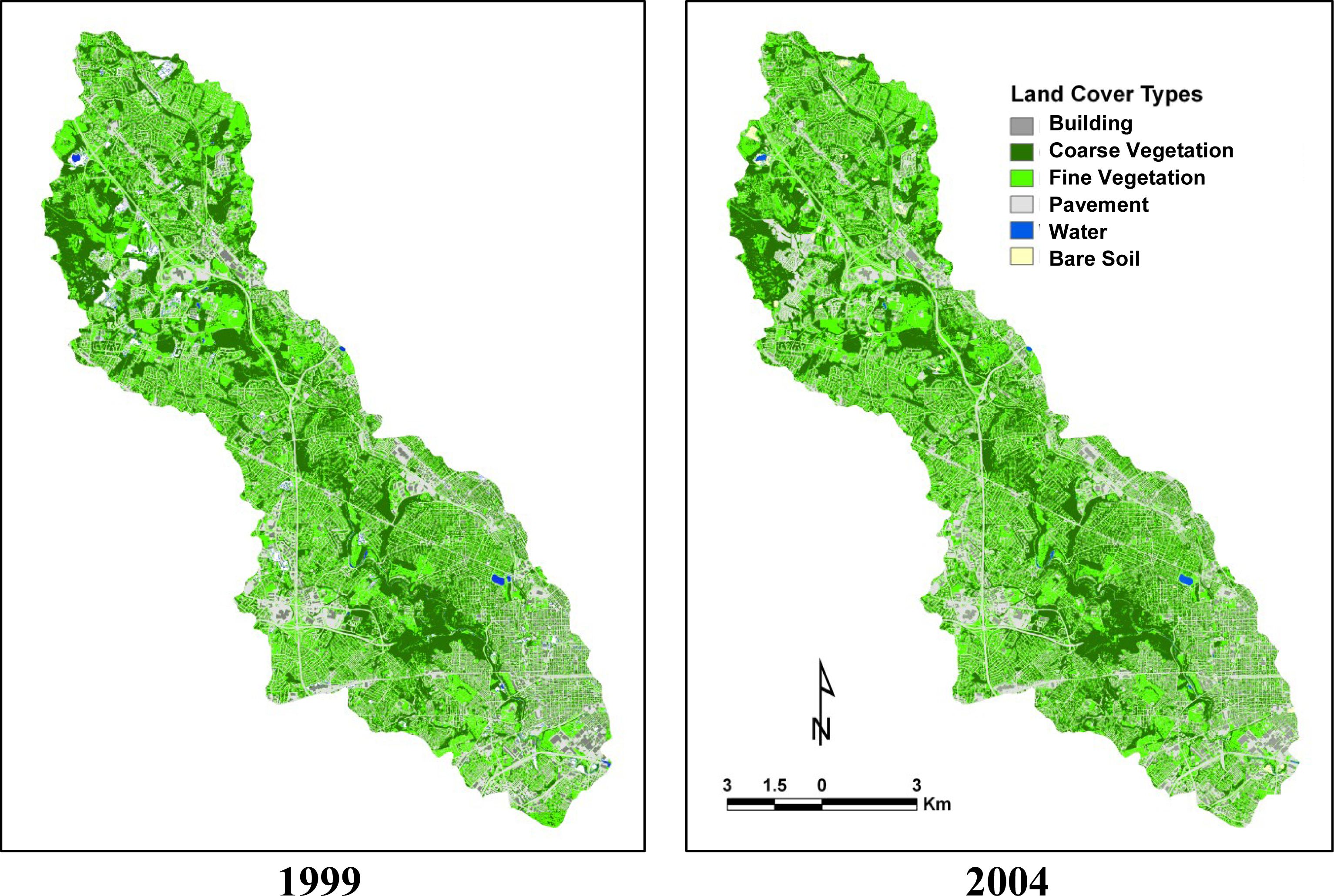
4], which will be discussed in detail in the method section. These patches serve as pre-defined boundaries for finer-scale segmentation and classification of within-patch land cover features, using an object-based classification. Patches are then classified based on the within-patch proportion of land cover features. We applied this approach to the Gwynns Falls watershed in Baltimore, Maryland, USA for two years, 1999 and 2004 to quantify the fine-scale heterogeneity and understand change over time.
2. Methods
2.1. Study Site
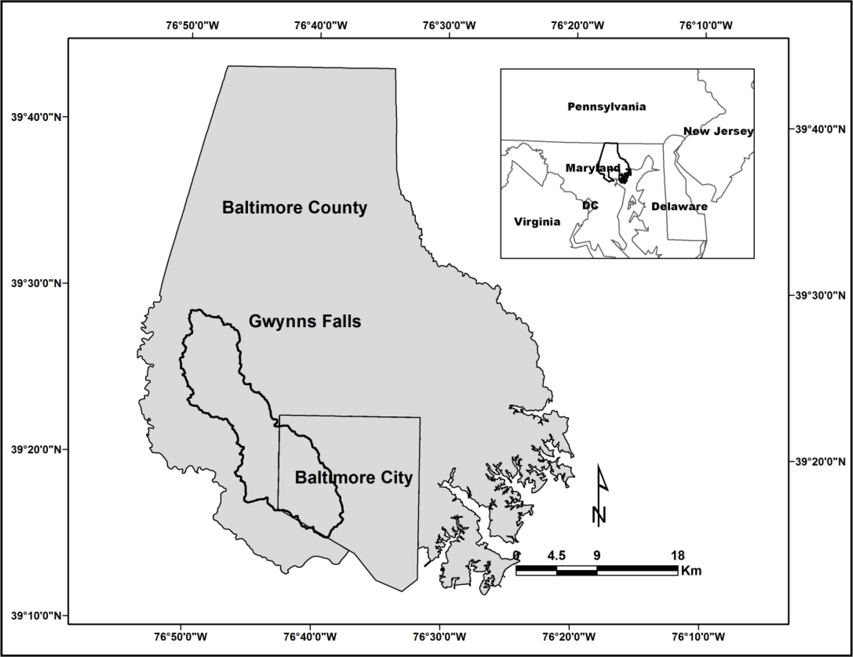
This analysis was conducted for the Gwynns Falls watershed, one of the focal research watersheds of the Baltimore Ecosystem Study (BES), a long-term ecological research project (LTER) (
www.beslter.org). The Gwynns Falls watershed, approximately 17,150 hectares in size, spans Baltimore City and Baltimore County, Maryland, USA and drains into the Chesapeake Bay (
Figure 1). It traverses an urban–suburban–rural gradient from the urban core of Baltimore City, through older inner ring suburbs to rapidly suburbanizing areas in the middle reaches and a rural/suburban fringe in the upper section. Land cover in the watershed varies from highly impervious in lower sections to a broad mix of uses in the middle and upper sections.
2.2. Data
Data used in this study included: (1) high spatial resolution color-infrared digital aerial image data for two years (October 1999 and August 2004); (2) Light Detecting and Ranging (LIDAR) data acquired in March 2002; and (3) building footprints (ca. 1997). The aerial imagery was used for both patch delineation and within-patch land cover classification, while LIDAR data and building footprints were only used to aid in the land cover classification.
The imagery was 3-band color-infrared, with green (510–600 nm), red (600–700 nm), and near-infrared (NIR) bands (800–900 nm). The imagery has a spatial resolution of 0.6 m, with an 8-bit radiometric depth. It was orthorectified using a bilinear interpolation resampling method, and it meets the National Mapping Accuracy Standards for scale mapping of 1:3000 (3-m accuracy with 90% confidence).
A surface height model was derived from the LIDAR data, and used to aid in the land cover classification. Both the first and last vertical returns were recorded for each laser pulse, with an average point spacing of approximately 1.3 m. The returns from bare ground and nonground (e.g., canopy, building roofs) were separated. The point-sample elevation data were interpolated into 1-m spatial resolution raster Digital Surface Models (DSMs) using the Natural Neighbor interpolation method available in ArcGIS 3D Analyst TM. Digital surface models were separately created to represent the bare ground and nonground features from the return measurements. A surface cover height model was then generated by subtracting the bare ground DSM from the surface cover DSM.
Building footprints of Baltimore County and City of Baltimore (ca. 1997) were also used in this study. A limited assessment was conducted to compare the building footprints to the aerial image data. The building footprints appeared to agree spatially with the aerial imagery, but a considerable number of buildings that were constructed after 1997 were not captured.
2.3. Patch Delineation
The HERCULES land cover classification scheme was used to delineate patches. HERCULES classifies the biophysical structure of urban environments using six landscape features: (1) coarse-textured vegetation—trees and shrubs (CV); (2) fine-textured vegetation—herbs and grasses (FV); (3) bare soil; (4) pavement, (5) building; and (6) building typology [
4]). Building typology has five recognized types (
Table 1). Water is represented by the absence of the other elements.
HERCULES patches were digitized on-screen using the imagery in ArcGIS TM 9.2. Patches were delineated separately on the two datasets (1999/2004). Patches must be a minimum size of 20 m in two orthogonal directions to be recognized. This size constraint prevents: (1) roads, except for interstate highways and large divided roadways, from becoming independent patches; smaller roads and streets are included in the patches, and the variation among patches in the density of roads is captured by quantifying cover of paved surfaces; (2) individual parcels from being recognized as unique patches, as the land cover may reflect single land-owner management decisions; and (3) a single row of trees being recognized as unique patches.
The delineation of patches was an iterative process. Patches were mapped by two cycles of scale-explicit, rule-based interpretation of imagery, followed by QA/QC (quality assurance/quality control). Patches with no buildings were mapped first. These included patches of: (1) closed canopy woody vegetation; (2) open canopy; (3) major roads; and (4) water bodies. A patch of closed canopy woody vegetation is composed of continuous woody canopy with no built structures and an area larger than 0.5 ha. If there is an opening of greater than 20 m by 20 m, this opening will be mapped as a separated patch or patches. Patches of open canopy are those with no continuous canopy and no built structures; however, there may be isolated or scattered woody vegetation present. A road patch was mapped only if the width of the roads was greater than 20 m; examples are highways and major roads with multiple lanes. For those roads that were not wide enough to be delimited as an individual patch, if a road separates two patches, then the road is divided equally between the two patches; i.e., the patch boundary is drawn down the center of the road. Only water bodies with water year round were recognized as unique patches. This excluded ephemeral water bodies such as detention ponds.
Patches with built structures were then mapped based on the types of buildings recognized in the HERCULES classification (
Table 1). A patch was delimited to include only one type of building, and any spatially associated vegetation and paved surfaces. Spatially adjacent buildings with the same building type were mapped into one patch if the relative abundances of the spatially associated vegetation and paved surfaces were similar. Otherwise, separated patches would be delineated.
Following the delineation of the draft patches, a different interpreter revisited each patch. This process involves a closer inspection of patch content to determine the presence and relative amounts of the features that make up the patch. This closer inspection may have resulted in discovering that the draft patch needed to be split into two or more patches. More often, assessing the relative amounts of the features that make up the patch may have led to the realization that the draft patch contained the same elements in the same proportions as an adjacent patch, resulting in a merge of the adjacent patches. Often the similarity between patches was overlooked in the initial stage because the arrangement of the elements in the two patches was very different, making visual interpretation of cover challenging. In general, the tendency to merge rather than to split patches was consistent across the years sampled; however, this was not quantified.
2.4. Patch Classification
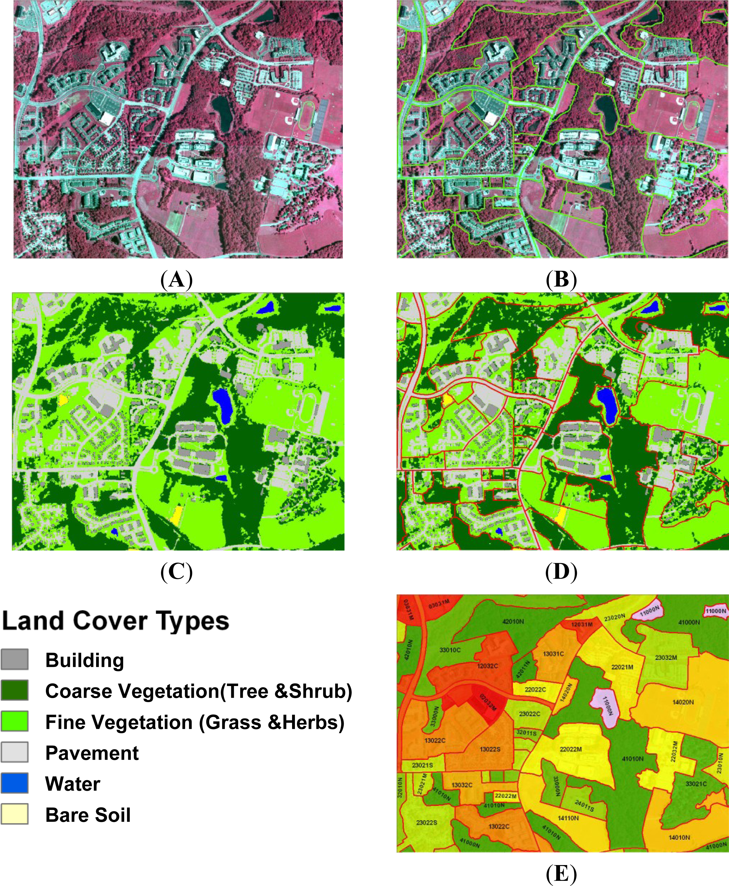
Following patch delineation, an object-based approach was used to classify those patches according to the HERCULES criteria—the six landscape elements identified above. We developed a two-level hierarchical classification system. Image objects were generated at two hierarchical scales: (1) patches (level 2, or higher level); and (2) land cover features within patches (level 1, or lower level). The delineated patches served as pre-defined boundaries for finer-scale segmentation and classification of within-patch land cover features. Classification of the five land cover features were performed first (
Figure 2, Panel C). Patches were then classified based on the within-patch, proportional cover of the five land cover features, combining building typology (
Figure 2, Panel E;
Table 2). We implemented this framework in Definiens Developer (now eCognition 8), an object-based image analysis program [
23]. Separate classifications were created for the two study years.
2.4.1. Classification of Land Cover Features
We first segmented the image into object primitives, which consisted of groups of relatively homogeneous pixels. These objects were the building blocks for subsequent classifications following the methodology discussed in more detail in a previous study [
20]. The image segmentation algorithm used in this study followed the fractal net evolution approach [
23,
24]. It is a bottom-up region merging algorithm, which is initialized with each pixel in the image as a separate segment. In subsequent steps, spatially adjacent segments are merged into a larger one if the increase in heterogeneity of the new segment compared to its component segments is less than a user-defined scale parameter [
24]. The scale parameter indirectly controls the size of objects by specifying the maximum heterogeneity that is allowed within each object: The greater the scale parameter, the larger the average size of the objects. User-defined color and shape parameters can also be set to change the relative weighting of reflectance and shape in defining segments. The process stops when there are no more possible merges given the defined scale parameter. The segmentation was conducted at a very fine scale, with a scale parameter of 20. The color criterion was given a weight of 0.9, while the shape was assigned with the remaining weight of 0.1, giving equal weights to compactness (
i.e., 0.05) and smoothness. The scale parameter of 20 and the values for the color and shape parameters were determined by visual interpretation of the image segmentation results, where objects were considered to be internally homogenous,
i.e., all pixels within an image object belonged to one land cover class [
20,
25].
Following the image segmentation, a rule-based classification,
i.e., a set of membership functions, was used to classify each of the objects into one of the five land cover features defined in HERCULES. A class hierarchy and its associated knowledge base of classification rules were developed by adapting the knowledge base created by a previous study [
20]. Here, we describe the class hierarchy, its associated features and rules, and the classification processes (
Figure 3).
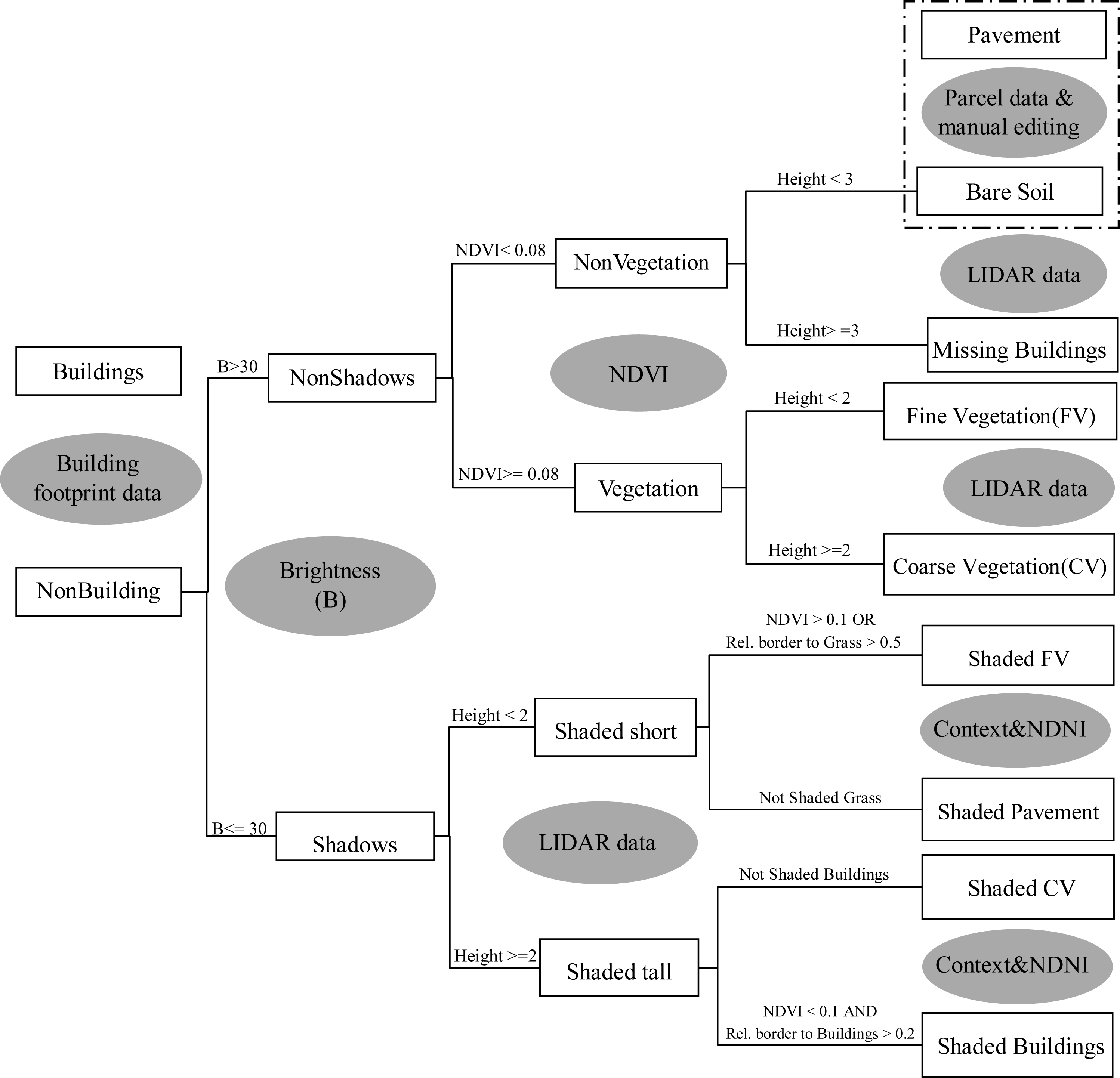
We first separated buildings from non-built areas by using the information from the thematic layer of building footprints. Then, the non-built areas were classified into areas with shadows and areas without shadows using brightness, with the threshold value of 30 determined by a histogram thresholding method [
20,
25]. The brightness was defined as the channel mean value of the three image layers,
i.e., green, red and near-infrared bands. The areas without shadows were further subdivided into vegetated areas and non-vegetated areas using Normalized Difference Vegetation Index (NDVI), which was derived from the red and near-infrared bands: Objects with NDVI values greater than 0.08 were classified as vegetation. Vegetation was further divided into coarse vegetation and fine vegetation, based on the height information obtained from the surface height model generated from LIDAR. Non-vegetated areas with height values of greater than 3 m were classified as buildings. We added the class of “missing building” to compensate for the fact that buildings built after 1997 were missing from the building footprint dataset. The parcel boundary layer contained information regarding the year of housing construction which was used to separate pavement from bare soil, as bare soil was mostly associated with new construction. Manual editing was further conducted to improve the separation of bare soil from pavement.
Before we further classified shaded objects, we performed an additional segmentation at a finer scale on the shaded objects, using the value of 5 for the scale parameter [
25]. Shaded objects were then classified into tall and short objects, using information from the surface height model. Short objects were further distinguished into shaded fine vegetation and shaded pavement using both NDVI and spatial relations to neighboring objects. Shaded fine vegetation included objects with an NDVI value greater than 0.l or whose relative “borders to fine vegetation” value was greater than 0.5. The value of “borders to fine vegetation” was defined as the ratio of an object’s border shared with neighboring fine vegetation objects to the total border length. Shaded tall objects were classified as shaded buildings if their NDVI values were less than 0.1 and their relative borders to buildings were greater than 0.2; otherwise they were classified as shaded trees.
2.4.2. Accuracy Assessment on Classification of Land Cover Features
Accuracy of the land cover classification was assessed separately for the two years. We used pixels as the assessment units [
26]. For each classification map, a stratified random sampling scheme based on the mapped land cover classes as strata was used to generate random points [
27]. A total of 350 points were sampled, with a minimum of 50 random points representing each of the five land cover features [
17,
27]. The 1999 and 2004 imagery were used as reference data. In addition, natural color orthophotos with spatial resolution of 0.3 m that were collected in 2005 were used, in cases a decision could not be made only based on the 1999 or 2004 imagery (e.g., the randomly selected checking point was under shadow). An error matrix was created for each classification map. We calculated the overall, and user’s and producer’s accuracies based on the error matrices (
Table 3). We incorporated the inclusion probabilities for the stratified design when calculating the user’s and producer’s accuracies [
26].
2.4.3. Patch Classification
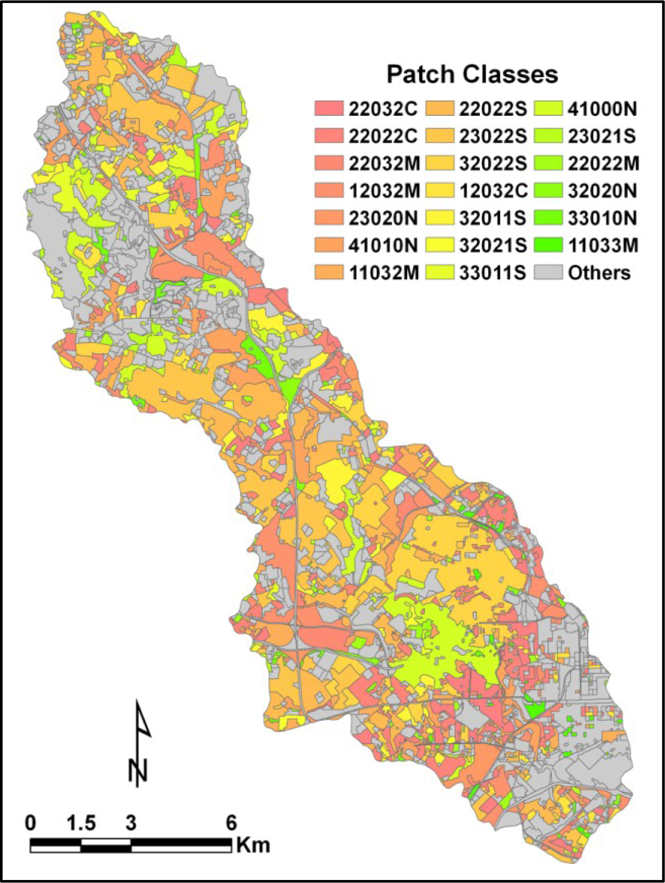
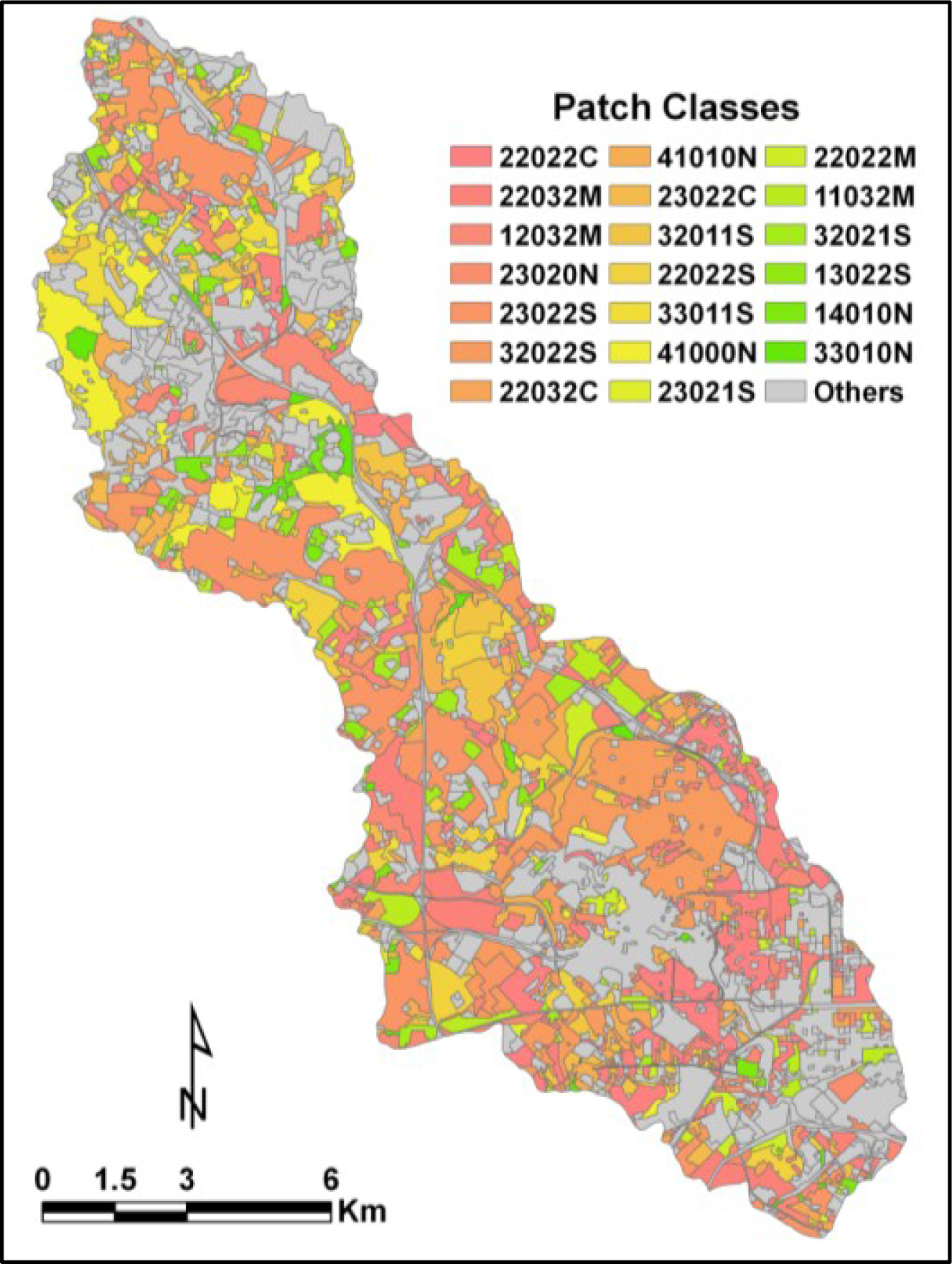
Patches, the objects at the higher level, were classified based on the within patch proportion cover of the five land cover features, combining building typology. The within-patch proportion cover of the five land cover features was obtained using the information from the sub-objects in the lower level. The proportional cover is divided into five categories: (0) absent, (1) present to 10% cover, (2) 11%–35% cover, (3) 36%–75% cover, and (4) >75% cover [
4]. Building typology was visually interpreted during the process of patch delineation. Patch classes are defined by combining the proportion cover of all the five land cover features and building typology within each patch (CV + FV + Bare Soil + Pave + Building + Building type). For example, a patch with a high proportion of coarse vegetation (>75%), medium density of single detached houses (11%–35%), little fine vegetation and pavement (present to 10%), and no bare soil, is classified as “41012S”. For an example of patches classified using HERCULES see
Table 2.
4. Discussion
Urban areas are strikingly heterogeneous. To develop an ecological understanding of urban systems, it is critical to quantify the fine-scale heterogeneity of their built and natural components. Recent availability of high-spatial resolution satellite and aerial imagery provides new opportunities to describe and quantify this fine-scale heterogeneity. However, it also calls for new approaches geared towards such data. In this study, we present an approach that combines visual interpretation and object-based image analysis to describe and quantify the fine-scale heterogeneity in urban landscapes. By integrating the strength of visual interpretation in patch delineation with an object-based approach in patch classification, this new approach provides an effective way to quantify the structure of urban landscapes that will better accommodate ecological research linking system structure to ecological processes. Our results showed that the urban landscape is very heterogeneous, characterized by extreme fine-scale patchiness and large variability in patch size.
4.1. Patch Delineation and Patch Classification: Visual Interpretation versus Digital Image Processing
Patch Delineation. Visual interpretation is superior to digital processing methods in delineating patches, even with the great recent advances made in object-based image analysis techniques [
8,
21,
22]. In fact, objects generated from image segmentation are mostly image objects without realistic ecological meaning [
19,
22]. Humans are exceptionally adept at visually recognizing and interpreting complex spatial patterns [
13,
14]. In particular, ecological knowledge can be integrated into image analysis through visual interpretation with ease, but ecological knowledge is difficult to incorporate into digital image processing techniques (Jensen 2000 [
14]; Richards and Jia 2006 [
6]; Lang 2009 [
8]). Incorporating ecological knowledge into patch delineation is critical in measuring and quantifying the fine-scale heterogeneity in urban landscapes. Therefore, incorporating ecological knowledge makes visual interpretation valuable for patch delineation, even though it is labor-intensive, and thus expensive.
Recent advances in object-based image analysis greatly enhance our capacity in urban land cover classification and feature extraction [
19,
21]. With the development of object-based image analysis, there is increasing interest in the automatic delineation of ecologically realistic objects [
8,
22,
29].
The integration of future advances in image segmentation with knowledge-based classifications may allow us to incorporate ecological knowledge with ease, allowing for the automatic delineation of ecologically meaningful objects, or patches [
8,
22].
Patch Classification. Recent advances in object-based image analysis allow an automated quantification of land cover features at fine spatial scales [
19–
21]. Our results show that an object-based approach provides an effective way for the classification of land cover features within a patch, and thus for patch classification. Therefore, an integration of the strength of visual interpretation for ecological patch delineation, and the effectiveness of an object-based approach for patch classification, provides a better way than using visual interpretation or an object-based approach alone, in quantification of fine-scale heterogeneous urban landscapes [
8,
30].
Alternatively, the within-patch proportion of land cover features can be visually estimated [
4], in case there are no resources to perform object-based classification. Visual interpretation, however, is relatively poor in quantification of the finer scale of within-patch land cover features, compared to digital processing methods such as object-based image analysis [
6,
15]). A comparison between the estimates from visual interpretation and those from object-based classification showed that estimates by visual interpretation are moderately accurate, with overall accuracies varying by land cover features [
15]. While visual interpretation does not work effectively when patches contain a mix of different types of features, accuracy increases with patches that are either dominated by a specific feature, or do not contain a specific feature [
15].
An object-based approach, however, not only provides more accurate patch classification, but also provides more flexibility in patch classification. Different classification schemes, unlike the one used for patch classification in this study, can be developed based on different research questions. For example, if research needs require more or less categorical resolution in land cover features, the classes can be easily obtained by recoding the continuous percent cover of the land cover feature(s) within a patch.
4.2. Advancing Our Understanding of Ecological Processes in Cities
In addition to describing and quantifying the fine-scale heterogeneity in urban systems, this integrative approach also provides a tool for: (1) Communicating with and collaborating with other disciplines such as social science and urban design to implement integrated socio-ecological research; (2) stratifying the landscape to assist with sampling schemes design and site selection; (3) testing hypotheses for structure-function links; and (4) exploring hierarchical patch dynamics. Integrated socio-ecological research requires a match between the spatial and categorical resolution of ecological and social datasets [
31]. For example, household level social data would be of little use to ecologists who may only be able to say something about urban land cover at the scale of the watershed and vice versa. In addition, the integration of built and non-built areas into ecologically relevant patches may also correspond to patches of social significance. For example, neighborhoods that were built at the same time will likely have similar amounts of fine vegetation, coarse vegetation, and building cover especially if they were built by the same developer. Neighborhoods with similar structure would be captured as a single HERCULES patch. This patch may also represent social organization in the community, for example, a neighborhood association, which could affect the relative proportion of cover by implementing management decisions. Classifications that do not integrate built and non-built components would not be able to capture this reciprocal relationship.
The flexibility of the classification also makes it well suited for stratifying the landscape to assist with sampling schemes design and site selection. The hierarchical nature of the classification allows patches with similar land cover proportions to be selected. For example, if a research question addressed forest patches embedded in the city, an investigator could select patches in the classification with continuous woody vegetation. Alternatively, a researcher might be interested in testing the affect of lawn age on carbon cycling. The flexibility of the classification would allow the investigator to select lawns of a different age while keeping all other factors constant (e.g., herbaceous vegetation, woody vegetation, and building cover). It also allows for the testing of gradients of land cover, for example, a researcher could select patches with three different densities of building cover while holding woody vegetation constant.
By separating ecological structure from function, this integrative approach also provides a tool for testing hypotheses of structure-function links in cities [
32,
33], a research area ripe for expansion and relevant as the Earth becomes increasingly urban. Finally, the hierarchical nature of the classification permits the exploration of patch dynamics as well as within-patch variation when temporal data are available. For example, by quantifying how much change of within-patch land cover feature will lead to changes in HERCULES patches, we can examine how changes in HERCULES patches link to those in within-patch land cover features.
5. Summary and Conclusions
Urban areas are inherently heterogeneous. To develop an ecological understanding of urban systems, it is critical to quantify the fine-scale heterogeneity of their built and natural components. This paper presents a new approach to quantify and measure the fine-scale heterogeneity in urban systems using high-spatial resolution imagery. This approach combines visual interpretation for patch delineation, or delimiting ecologically meaningful objects, with an object-based image analysis approach to quantify the land cover features within patches for patch classification. It integrates the strength of human interpretation in patch delineation and the effectiveness of an object-based approach in automated quantification of finer-scale land cover features. This approach provides a more efficient and ecologically meaningful way than either purely automated or visual methods alone to measure and quantify the structure of urban systems, using high-spatial resolution remotely sensed imagery. In addition, it also provides a useful tool for site selection, testing hypotheses linking structure of urban systems and ecosystem function, and integrated socio-ecological research.


