Abstract
Water authorities are required to have a survey of large woody debris (LWD) in river channels and to manage this aspect of the stream habitat, making decisions on removing, positioning or leaving LWD in a natural state. The main objective of this study is to develop a new methodology that assists in decision making for sustainable management of river channels by using generated low-cost, geomatic products to detect LWD. The use of low-cost photogrammetry based on the use of economical, conventional, non-metric digital cameras mounted on low-cost aircrafts, together with the use of the latest computational vision techniques and open-source geomatic tools, provides useful geomatic products. The proposed methodology, compared with conventional photogrammetry or other traditional methods, led to a cost savings of up to 45%. This work presents several contributions for the area of free and open source software related to Geographic Information System (FOSSGIS) applications to LWD management in streams, while developing a QGIS [1] plugin that characterizes the risk from the automatic calculation of geometrical parameters.
1. Introduction
Trees that grow along a stream often fall into the water course due to flooding, erosion, windfall, disease, beaver activity or natural mortality. These materials, often referred to as large woody debris (LWD), can include whole trees with the root mass and limbs attached or portions of trees with or without wads and branches. LWD significantly influences the structure and function of small headwater streams. However, what it contributes to the geomorphic function depends on where it is located relative to the stream channel and the size relative to the channel [2]. In addition, LWD can increase stream habitat heterogeneity by providing structure, altering flow patterns, enhancing sediment deposition, forming pools and retaining organic matter [3,4]. Thus, LWD removal should only be considered when there is compelling evidence that it could cause flooding of public or private infrastructure, significant stream bank erosion or could become a navigational hazard. However, one significant outcome of LWD research since the 1970s has been a more complete appreciation of fallen trees as an integral component of river and floodplain ecosystems, where they play a variety of physical and ecological roles. A complete literature review of LWD in river channels can be found in [5]. An overview of the different roles that woody debris plays in streams, in terms of pros and cons, can be found in [6,7,8,9].
The reasons for removing or relocating LWD, described by the above mentioned authors, include:
- Reduction of effective channel section, decreasing the natural capacity to transport water and increasing the risk of flooding.
- River stabilization; previously, LWD was believed to impair river stabilization by causing scouring of the river bed. However, recent research has shown that strategic placement of LWD can actually stabilize river banks and reduce erosion.
- River navigation; LWD can be hazardous to river navigation.
- Flood mitigation; LWD may hinder water flow and cause flooding in some situations (for example, where large debris dams are formed). However, in most cases, removal results in minimal improvement of channel capacity and a reduction of flooding in lowland rivers. LWD, particularly large tree trunks within the channel, was previously thought to impede water flow and result in additional flooding. We now know that a channel needs to be substantially blocked by LWD before there is any measurable effect on the water level. For example, at a particular location on the channel, the cross-sectional area of LWD needs to be at least 10% of the whole channel before a significant effect on water levels is likely [10].
- Human use; LWD in the riparian zone is often removed for firewood collection, agricultural purposes and other activities.
Water authorities are required to survey existing LWD in river channels and to make decisions on removing, repositioning or leaving LWD in their current location and position. This decision will be made considering an established management strategy. It is also important to evaluate riparian vegetation, which can play a key role in the propagation of flood waves [11].
Knowledge of channel slope, width, entrenchment, sinuosity and substrate combined with the length and diameter of the logs in the obstruction will provide a basis for determining whether the woody debris can be salvaged for creating log sills, deflectors or cover habitat or if it should be removed from the floodplain. Channel width will indicate the size of woody material that can be considered stable in the stream, and proper positioning in relation to flow can be determined.
A manual method for the LWD survey is described by Schuett-Hames et al. [12]. In this study, a methodology to automatically classify LWD depending on their level of riskiness was developed. Furthermore, along with the detection, the LWD was classified with an index as a function of their effect on the course. This index considers the LWD length, its relative position in the river course, the percentage that LWD occupies in the section of the channel and the accumulation of LWD in an area.
A remote sensing system can acquire satellite, airborne or ground-based images. The major difference among the three platforms is their viewpoint height, which dominates the spatial resolution and image field of view [13]. In the past 25 years, a considerable amount of research and development has been performed on airborne and space-borne, multispectral and hyperspectral imaging systems for use in water resource management [14]. Dunford et al. [15] analyzed the potential and constraints of using unmanned aerial vehicles (UAV) for the characterization of riparian forests. The main disadvantage of UAVs is the flying ability over narrow rivers with riverine frost and the flying regulations [16]. Additionally, UAVs are unsuitable for the area dimensions of the study case (more than 100 km) due to limitations regarding battery autonomy.
The detection of LWD in rivers requires high spatial resolution of the images obtained, as well as capturing the images on a specified date for the detection of LWD. These requirements make it difficult to find existing products in the market at an affordable cost. Marcus et al. [17] employed lower spatial resolution hyperspectral images (1 m) for mapping woody debris. In Lejot et al. [18], a set of very high resolution images in the visible spectrum were employed for river bathymetric purposes.
The main objective of this work was to develop a new methodology that assists with decision making for sustainable management of river channels by using newly generated low-cost, high-resolution geomatic products to detect LWD. The proposed methodology was evaluated through its application to a case study located in Spain, where an inventory of the LWD in a 132-km segment of the Júcar River was required.
2. Materials and Methods
A georeferenced, geometric product was used to determine the location of LWD, which was generated with aerial images of sites where LWD was detectable. Figure 1 shows an outline of the proposed methodology to obtain this type of product at a low cost. In every step, only open-source software was utilized. The process is fully described throughout the paper.
2.1. The Case Study
The case study (Figure 2) was the medium stretch of the Júcar River, downstream of the Alarcón Dam. The length covered by the experimental case was 25% of the total length of the river (132 over 512 km).
The river channel is well defined and bordered by riparian vegetation. The channel width varies between 10 and 30 m and the average slope between 0.1%–0.2%. The drainage area in this section covers an area of 6300 km2 of the 42,832 km2 of the Júcar River Basin. Its river bank is occupied by agricultural and urban uses.
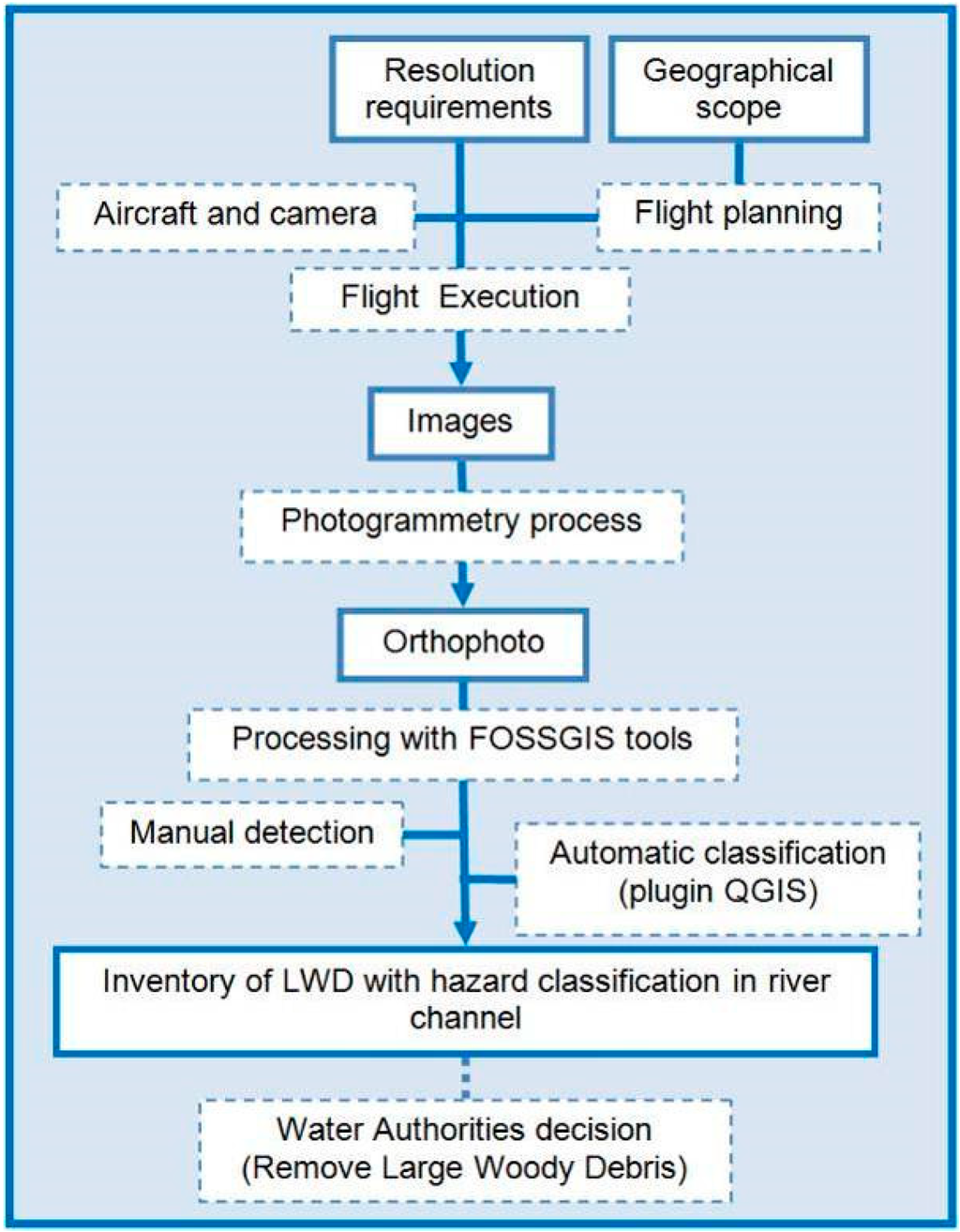
Figure 1.
Main flowchart of the proposed methodology. (Dashed line: flux or process; Continuous line: data and newly generated products).
Figure 1.
Main flowchart of the proposed methodology. (Dashed line: flux or process; Continuous line: data and newly generated products).
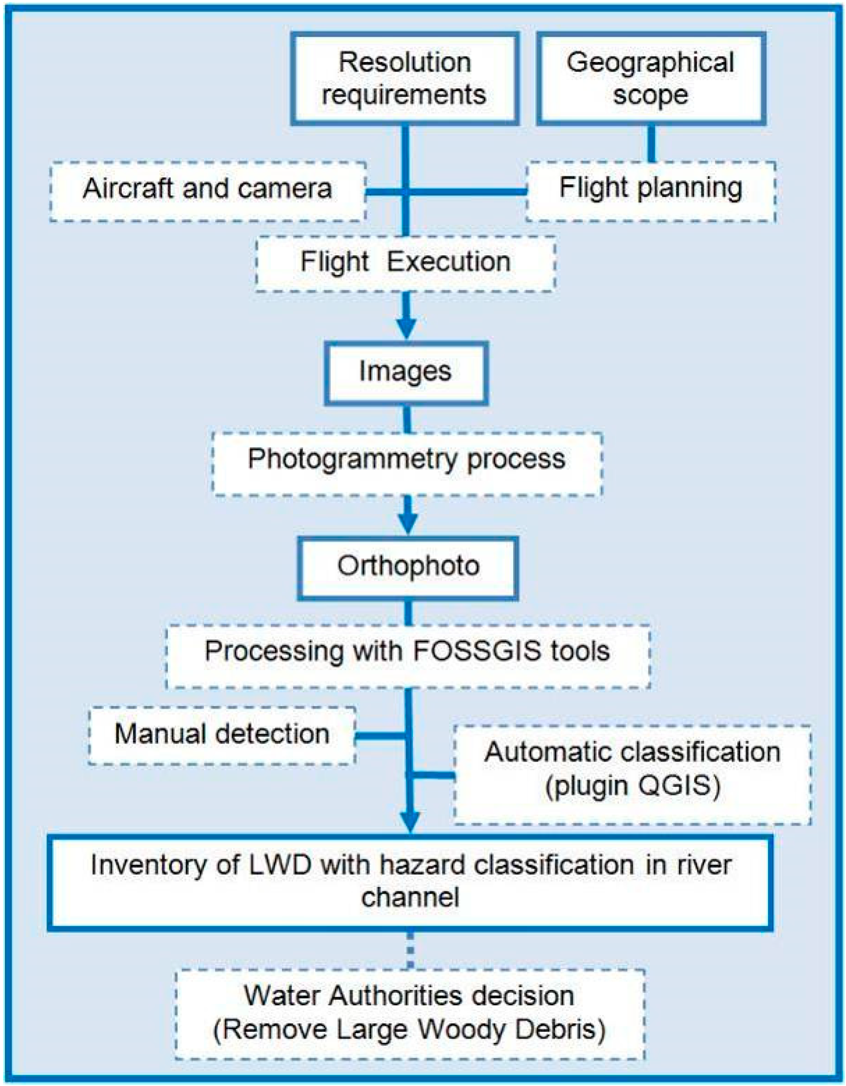
Figure 2.
Location of the case study (green area).
Figure 2.
Location of the case study (green area).

Water resource management of river basins in Spain is a duty of the Watershed Authorities (Confederaciones Hidrográficas), in this case the Júcar Watershed Authority (JWA). The JWA is responsible for assessing waterways for potential flooding. Traditionally, the JWA managed the removal or relocation of LWD when these elements were found by the field staff of JWA, as well as citizen groups, ecologists, police, etc. Once the notification was received, three operators and a skidder cleared the riparian vegetation and removed or relocated the LWD.
To avoid the risk of flooding, the JWA required the detection of LWD along 135 km and to remove or relocate it for sustainable management of the river channel. To do so, two options were initially considered: (1) ground inspection and (2) inspection by boat. The first option was rejected due to difficulty in river bank access, because riparian vegetation makes it difficult to directly detect LWD. To perform ground inspection, it would be necessary to clear out some of the riparian vegetation, which is not beneficial to river functioning and would generate a great environmental impact. The second option was rejected, because in this river, there are many artificial transversal structures. Thus, a georeferenced geomatic product with a high spatial resolution was planned for visually locating LWD, determining their position and then making decisions on the removal or relocation, with minimal disturbance to riparian vegetation.
2.2. Requirements of the Geomatic Product and Available Products
Geomatic products are characterized by their spatial, spectral, radiometric and temporal resolutions [19,20,21]. For this research, the spatial and temporal resolutions are the most important attributes. The spatial resolution was limited to ground sample distance (GSD) = 0.10 m, which is considered sufficient to detect LWD with a width of 30 cm (three times the GSD to eliminate neighbor effects [22]). Higher GSD values, to improve the spatial resolution, would not provide any additional significant benefit in LWD detection. However this overestimated spatial resolution will imply in the flight planning stripes with side overlap, which in conjunction with the sinusoidal river path, will increase processing time and final economic cost. The temporal resolution is established by considering three main aspects: (1) the images should be obtained after leaf abscission of the riparian vegetation, to facilitate detection of LWD; (2) images should be obtained close to the time the field work can be performed; and (3) the work should not be performed between March and July, the reproductive period of birds in the area, to avoid affecting bird populations when equipment is flown at low altitude. Regarding spectral resolution, the visual spectrum was selected for visually detecting LWD. Thus, the images were captured with a conventional compact camera, with a resolution of 1 byte in each of the three bands (red, green and blue). Precision in the georeferencing process is not a limiting factor, because the objective of this study was to provide workers with the location of the elements to be removed or relocated, for which a precision of 2 m is more than enough.
After performing a search for the geomatic products available for this area of interest, none fulfilled the specified requirements. Satellite-based products do not reach the required spatial resolution, with the highest resolution at 0.50 m [23]. The photogrammetric products available do not fulfill the spatial and temporal resolution. The orthoimage of the National Plan of Aerial Ortho-photography (PNOA) in Spain has a spatial resolution of 0.25 m, but the most recent product was dated July 2009, in which there was lush riparian vegetation, and the timing was far from the scheduled time for field work.
The final decision was to obtain a new orthoimage that fulfilled the requirements of this application, at a minimum possible cost. High resolution orthoimages are conventionally generated with images captured with a calibrated, photogrammetric digital camera mounted on a standard-sized airplane [24]. However, advances in computational vision and the new low-cost positioning (GNSS) and inertial movement units (IMU) make it possible to obtain low-cost orthoimages generated from images captured with an economical, non-metric digital camera mounted on a low-cost aircraft [19].
The proposed solution consists of flying a tandem minitrike upon which a camera is mounted on an auto-leveling platform. Similar solutions have been proposed in other studies [18,25,26]. By applying the photogrammetry workflow [27,28] to the images obtained using open source tools, the resulting orthoimage was georeferenced using control points of existing geomatic products. The alternative of using an unmanned aerial vehicle (UAV) was rejected, since the autonomy of this type of equipment is limited [29].
The geomatic information required for the flight planning process was freely obtained from the National Center of Geographic information in Spain [30]:
- PNOA 2009 orthoimage, with a GSD = 0.25 m and mean square error (MSE) = 0.5 m.
- Digital terrain model (DTM) with a 5-m grid and 2-m accuracy.
The final product was georeferenced considering the Coordinate Reference System (CRS) ETRS89 UTM 30 (EPSG Code 25830), which is required by Spanish law in all geomatic products. In the navigation phase, which uses a GPS, WGS84 CRS was utilized (EPSG Code 4326).
2.3. Description of the Aircraft and Payload Utilized
The aircraft was a tandem trike AIRGES minitrike (Figure 3) with the following characteristics: motor, Rotax 503 two-stroke motor; paraglider MAC PAR A Pasha 4 Trike; emergency system ballistic parachutes GRS 350; weight, 110 kg; and air velocity range 30–65 km/h.
Figure 3.
Camera mounting platform and details of the aircraft and the navigation system.
Figure 3.
Camera mounting platform and details of the aircraft and the navigation system.

The camera mounting platform (Figure 3) was similar to others described in the literature [18]. It consists of an aluminum platform with two servos that allow the operator to automatically keep the camera in a nadiral position. To do so, hardware and software were developed by the authors. The hardware consisted of an Arduino board with a 16-MHz Atmega 328 processor, which incorporated an inertial measurement unit (IMU) with the following sensors: three-axis accelerometers ADXL335 (range 3.6 g), two-axis gyroscope (x, y) LPR530AL (range ±300°∙s−1) and one-axis gyroscope (z) LY530ALH (range ±300°/s). The software developed was based on Quad1_mini V 20 software [31], with DCM (direction cosine matrix) as the management algorithm of the IMU [32]. Two FUTABA S3003 servomotors were installed to keep the camera in the nadiral position, with an accuracy of 6 DEG degrees.
The navigation system was composed of an ARMOR X10gx Rugged Tablet Computer, with a GPS Ublox EVK-6T-0 (Hybrid GPS/SBAS engine (WAAS, EGNOS, MSAS) single frequency (L1)). The GPS accuracy was 9 m on the horizontal axis and 15 m on the vertical axis for 95% of the time [33]. The GPS antenna (Trimble Bullet III) was installed on the camera platform close to the optical center of the camera (Figure 3).
In order to improve the altitudinal precision of the GPS, a DigiFly VL100 barometer was installed, obtaining an accuracy of 8 m. Thus, horizontal positioning during the flight was performed by following a track in a QGIS project file containing the shape files of the flight route and the NMEA (National Marine Electronics Association) position of the GPS system using RTKNAVI software [34]. The vertical positioning was performed by fitting the barometer readings to the planned flight. The error when fitting the flight execution to the planned flight, under favorable climate conditions, depends on the aircraft characteristics and pilot experience. In this case, this error was estimated as 5 m on both the vertical and horizontal axes. The final error considered the navigation and flight execution errors (quadratic error). The total error in the flight positioning was obtained by considering the error caused by the pilot (estimated at 5 m horizontally and vertically) and the error of the navigation system (9 m horizontally and 8 m vertically), resulting in 11 m horizontally and 10 m in altitude. This total error in the flight positioning is obtained by the quadratic composition of the mentioned error sources. The flight execution error was estimated based on previous flights comparing the planned vs. the executed flight obtained by means of the aerotriangulation process.
The camera utilized was a compact Olympus PEN EP1 camera (12.3 Megapixel Live MOS Sensor, 4032 × 3024; sensor geometric resolution, 0.0043 mm; and a wide-angle fixed focal 17-mm f2.8 lens), which has been used in other studies [35].
2.4. Flight Planning and Execution
In this case study, an area of 2657 km2 was covered. The flight planning process started with the definition of the study area described in the case study. The river axis was digitalized with a linestring using the PNOA orthoimage. This line defined the horizontal position of the aircraft. A buffer of 120 m from this line was applied to consider the whole area controlled by the JWA.
The total area of the polygon was 3240 ha. In this area, LWD was detected, as well as other characteristics of the morphology of the river banks, which could be useful in the decision making process.
Flight planning was performed by considering the relationship between the flight altitude over the DSM, the GSD and camera technical specifications. According to the characteristics of the camera, the maximum GSD required (0.1 m) and the error in altitude (10 m in this case), a flight altitude of 375 m was established with a GSD = 0.095 m. An error of 10 m in altitude positioning would lead to a GSD error of 0.003 m. Thus, in the worst scenario, GSD = 0.095 + 0.003 = 0.098 m would be obtained, which was lower than the required GSD. The 0.1-m GSD threshold does not meet a flight height of 395 m, which is larger than the conservative value for the aircraft altimetric error (Section 2.3).
Flight planning was performed considering that the camera mounting direction was coincident with the columns of the charge-coupled device (CCD) (4032 columns in this case). Thus, with GSD = 0.095 m, the length covered in each longitudinal flight was 383 m. This was more than enough to cover the required 240 m (120 m on each side of the center of the river), therefore being able to absorb the different errors from flight execution.
For obtaining an overlap of 60%, which is typical in conventional photogrammetry [24], the stereoscopic base should be 114 m. However, if the maximum nadiral positioning error is considered in two consecutive images, the base line should be decreased by 57 m (quadratic error of 40 m) to ensure this overlap value. Thus, a maximum flight speed of 14 m/s was established with a camera shooting interval of 4 s, which guaranteed a minimum overlap of 60%, adequate for the 3D process, although for the modern matching algorithms, the overlap value should reach up to 70%–80%. A shutter speed of 1/1000 s was adequate for this speed, because the equivalent terrain displacement would be 0.014 m, which is lower than 1/5 pixel, an insignificant value in photogrammetry. An ISO of 125 was used with a focal length of infinity.
The flight availability and execution was planned based on the NOAA weather models through the zyGrib software, in order to meet the weather requirements for the flight. These requirements go from a minimum wind speed, absence of rain up to the presence of turbulence resulting from thermal currents. The whole area was covered on three separate days. However, to facilitate photogrammetry post-processing, the whole set of images was divided into 82 blocks with a maximum linear length of 2400 m each. In addition, this avoids errors due to scaling factors when referencing the horizontal coordinates to the CRS 25830. The number of images per block varied between 33 and 39, and the length ranged between 1869 and 2214 m.
2.5. Photogrammetry Workflow
The first step was determining the approximate orientation of the images. The estimation of the optical center for each image was obtained with RTKLIB software [34] and GNSS information. These estimated positions were used in conjunction with the ground mean altitude to determine the overlapping images for the matching process improvement and as initial values for the bundle adjustment of the camera network.
In a conventional photogrammetry process [24], the control points must be measured with a precision higher than 1/3 of the GSD. In this case, it would require a precision of 0.03 m, which can only be obtained with GNSS-RTK techniques [36] with a high workload. However, in this case study, the required absolute precision for the georeferencing process was established at 2 m, which made it possible to measure the control points in available geomatic products. These measurements were taken with QGIS using the PNOA orthoimage and the DTM described above.
The generation of the photogrammetric model involved three different steps solved by Apero-Micmac modules [37]. Firstly, the images were matched by the SIFT algorithm [38], with 2000–2500 tie-points between image pairs. Secondly, the camera orientations were computed by the Apero Module [37] using the tie-points calculated in the previous step and the coordinates of the targets located on the ground in the flight area. Finally, a digital surface model (DSM) was obtained by means of ray intersection [24,37]. To solve this process, an SGM (semi-global matching) technique [39] was applied. Once the DSM was obtained, it was possible to generate an orthoimage for each of the images, which were combined to generate a complete mosaic.
Finally, although the precision required in this case study was lower than in conventional photogrammetry works, it was convenient to perform quality control. In this sense, the main problems of the final model were: (1) the generation of gaps in the orthoimage; (2) the generation of geometric artefacts; and (3) georeferencing errors. The first two sources of error were detected visually by using QGIS. The quality control of the georeferencing process was performed using a random cloud of 20 points in each of the 82 blocks. A set of 10 points from these 20 were selected, which were closer to the river axis. The x and y coordinates were measured in the model generated and in PNOA 25 cm, calculating the error in planimetry. Elevation tests were not performed, since these were not required in this study case.
2.6. Automatic Classification of LWD Using FOSSGIS Tools
The automatic risk parameterization of LWD was performed by developing a plugin for QGIS using the Python language. The agile QGIS cartographic editing tools of QGIS and the ability to quickly and easily extend its functionality by developing new plug-ins in the Python programming language adapted to the aims pursued justifies the adoption of this decision [16,40,41].
The implementation of the plugin required the configuration of the development environment for PyQGIS, preliminary operations and the development of the proposed feature following the Style Guide for Python Code PEP0008.
This plugin requires knowing the location and characteristics of each individual LWD. This information was manually digitalized as linestring in the generated orthoimage. In addition, it was required to digitalize the riverbanks’ limits, transversal barriers and the axis of the river channel. All of this information is stored in a SpatiaLite [42] spatial database (Figure 4).
Figure 5a,b shows an example of elements deposited in the channel from the visual inspection of the geomatic product. Figure 5c shows the common metric parameters that characterizes the level of risk of the LWD [43] on flooding, which was determined from the realization of a series of geometric calculations: (1) length of the LWD (distance AB); (2) distance of the barycenter (PM) of the LWD to the river axis (cyan line); (3) percentage that the LWD occupies of the transversal section of the river (red line); and (4) number of LWD individuals (brown lines) in the neighboring area (closer than 100 m).
After calculating these four parameters, an indicator of the riskiness of each LWD was calculated by weighting each of these parameters. The weighting coefficients were 0.2, 0.1, 0.5 and 0.2 for each of the four parameters, respectively. These weights were chosen according to the feedback of previous studies. This permitted classifying the LWD individuals regarding their level of risk and, therefore, making decisions about their removal or relocation, optimizing economic resources.
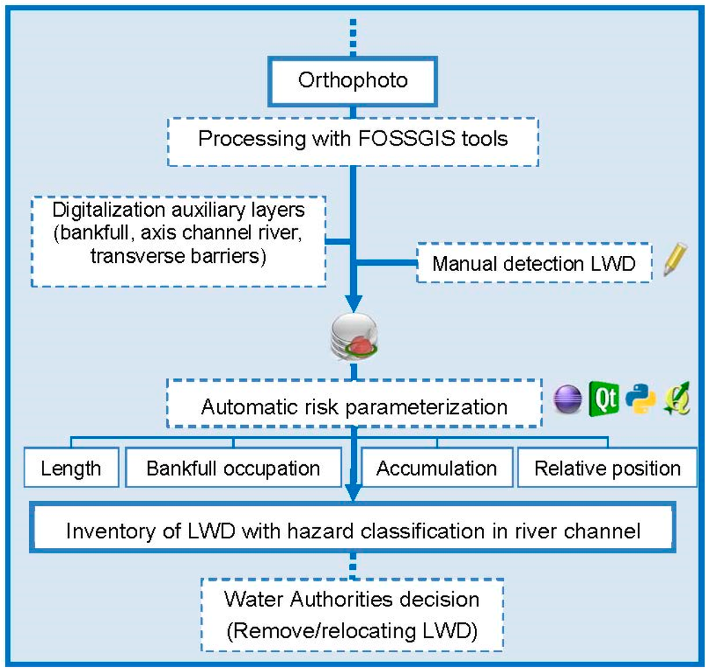
Figure 4.
Flowchart of the processing with FOSSGIS tools for obtaining an inventory of LWD with hazard classification in the river channel (dashed line: flux or process; continuous line: data and generated products).
Figure 4.
Flowchart of the processing with FOSSGIS tools for obtaining an inventory of LWD with hazard classification in the river channel (dashed line: flux or process; continuous line: data and generated products).
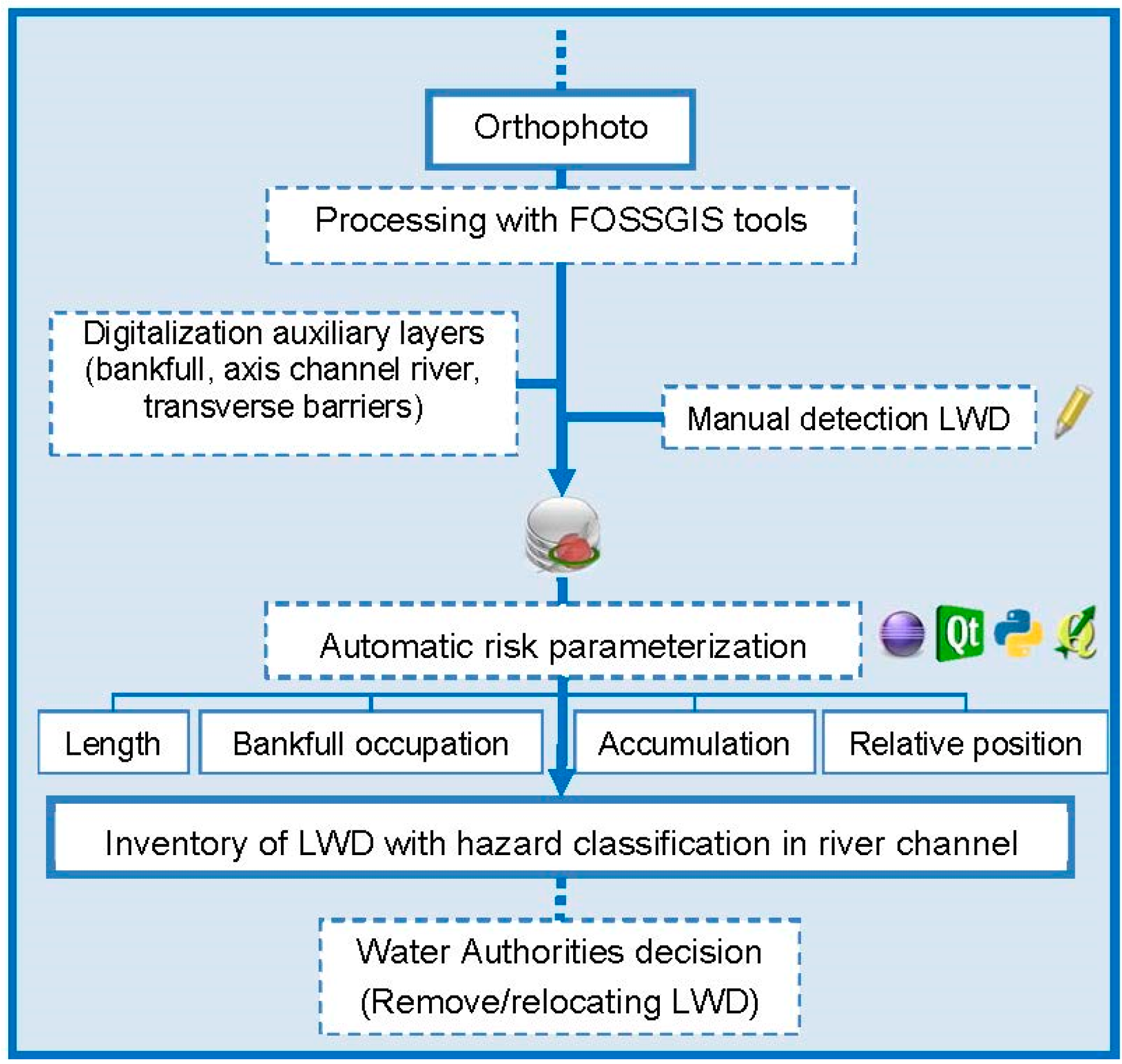
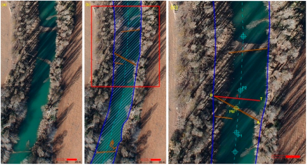
Figure 5.
(a) Section of the channel with LWD; (b) geometric characterization of the LWD and river channel; (c) metric parameters related to the risk level of the LWD.
Figure 5.
(a) Section of the channel with LWD; (b) geometric characterization of the LWD and river channel; (c) metric parameters related to the risk level of the LWD.

2.7. Economic Analysis of the Proposed Solution
To evaluate the proposed methodology from an economic point of view, three different methodologies for detecting LWD in river channels were compared with the proposed one.
- (1)
- The traditional method, consisting of removing riparian vegetation along the river to visually detect LWD. It is only applied in some problematic reaches of the river and consists of removing riparian vegetation every 50–60 m to detect LWD. Cost data from 2007 over a 4-km river segment were available.
- (2)
- Navigation by boat along the river and measuring LWD position using GPS; to evaluate the cost of this methodology, current tariffs were utilized. Based on previous experiences of JWA in similar tasks, a navigation rate of 1 km/h was considered, which therefore would require 132 h to navigate the segment analyzed. A 60 HP semi-rigid boat would be required.
- (3)
- Conventional photogrammetry, using conventional aircraft. The cost of performing this type of work was requested from different enterprises.
3. Results and Discussion
3.1. Adjustment of Flight Execution to the Flight Planning
The procedure yielded a total of 82 blocks and a total of 2960 images. The mean, maximum and minimum values of the main parameters of the flight are described in Table 1.

Table 1.
Results of the data processing.
| Parameter | Mean | Max | Min |
|---|---|---|---|
| Flight altitude (m) | 375.5 | 384.1 | 365.3 |
| GSD (m) | 0.095 | 0.097 | 0.092 |
| Base line (m) | 55.3 | 62.6 | 47.4 |
| Deviation from verticality (DEG) | 4.6 | 8.1 | 0.5 |
| Length of each block (m) | 2050.86 | 2213.13 | 1869.58 |
| Quadratic mean error in planimetry (m) | 1.46 | 1.82 | 0.61 |
For most cases, the values fit the flight planning basis. In a few cases in which the extreme values did not fulfill these bases, it was evaluated if 60% overlap was obtained, which was fulfilled in all cases. In Table 1, the deviation from verticality error represents the camera mounting platform deviation from the planned flight.
The error in the georeferencing process ranged between 0.61 and 1.82 m, fulfilling the requirement of 2 m of precision. These errors were obtained for each photogrammetric block with their corresponding orientations, employing clearly identifiable points.
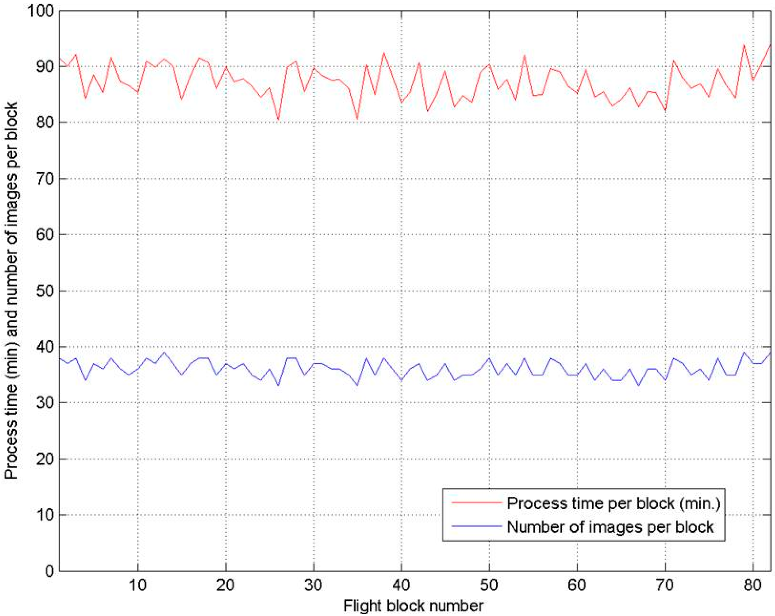
3.2. Processing Time
The processing time and the number of images processed for each block is represented in Figure 6. Obviously, the processing time is linearly related with the number of images of each block. The total time for processing all images was 120 h, using a laptop with an Intel Core i5-430M (2.26 2.52 GHz) processor and 4 GB RAM. Approximately 75% of the processing time was estimated to be automatic without requiring the supervision of the user.
Figure 6.
Process time and number of images per block.
Figure 6.
Process time and number of images per block.
3.3. Results of the Detection and Classification of LWD
With the obtained geomatic product, it is easy to detect the LWD deposited in the river channel. Additionally, using these products, it was possible to localize areas without riparian vegetation that would facilitate the access of machinery to the river to remove obstructive elements. The advantage of this procedure is the economic and environmental savings by avoiding vegetation removal. Figure 7 shows LWD detected in the orthoimage and the tree before its removal.
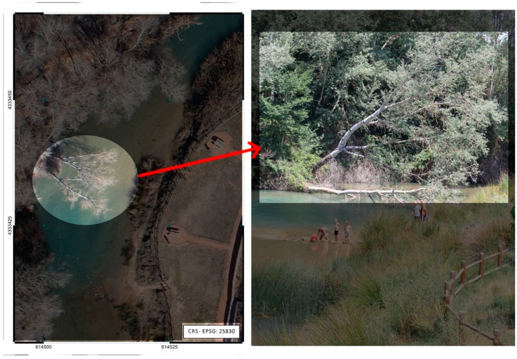
Figure 7.
LWD detected in the orthoimage and the tree before its removal.
Figure 7.
LWD detected in the orthoimage and the tree before its removal.
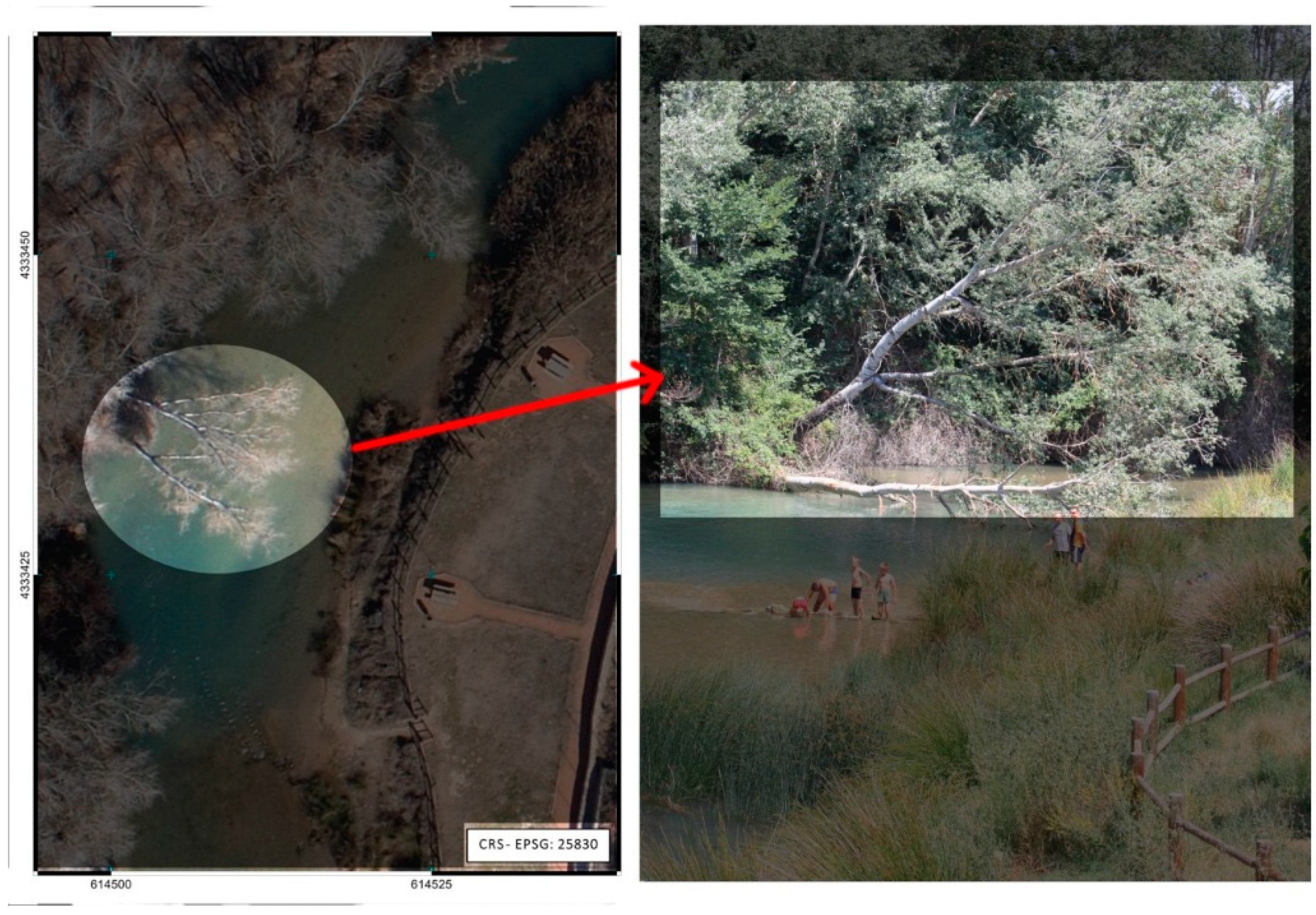
Figure 8 shows two different stretches of the Júcar River where LWD were detected. In the first reach, there was a high density of LWD detected, as well as LWD with different degrees of riskiness. However, in the other reach, the density was very low and with a low level of risk. Thus, this technique permitted detecting stretches with priorities of action (removing or relocating LWD to avoid flooding).
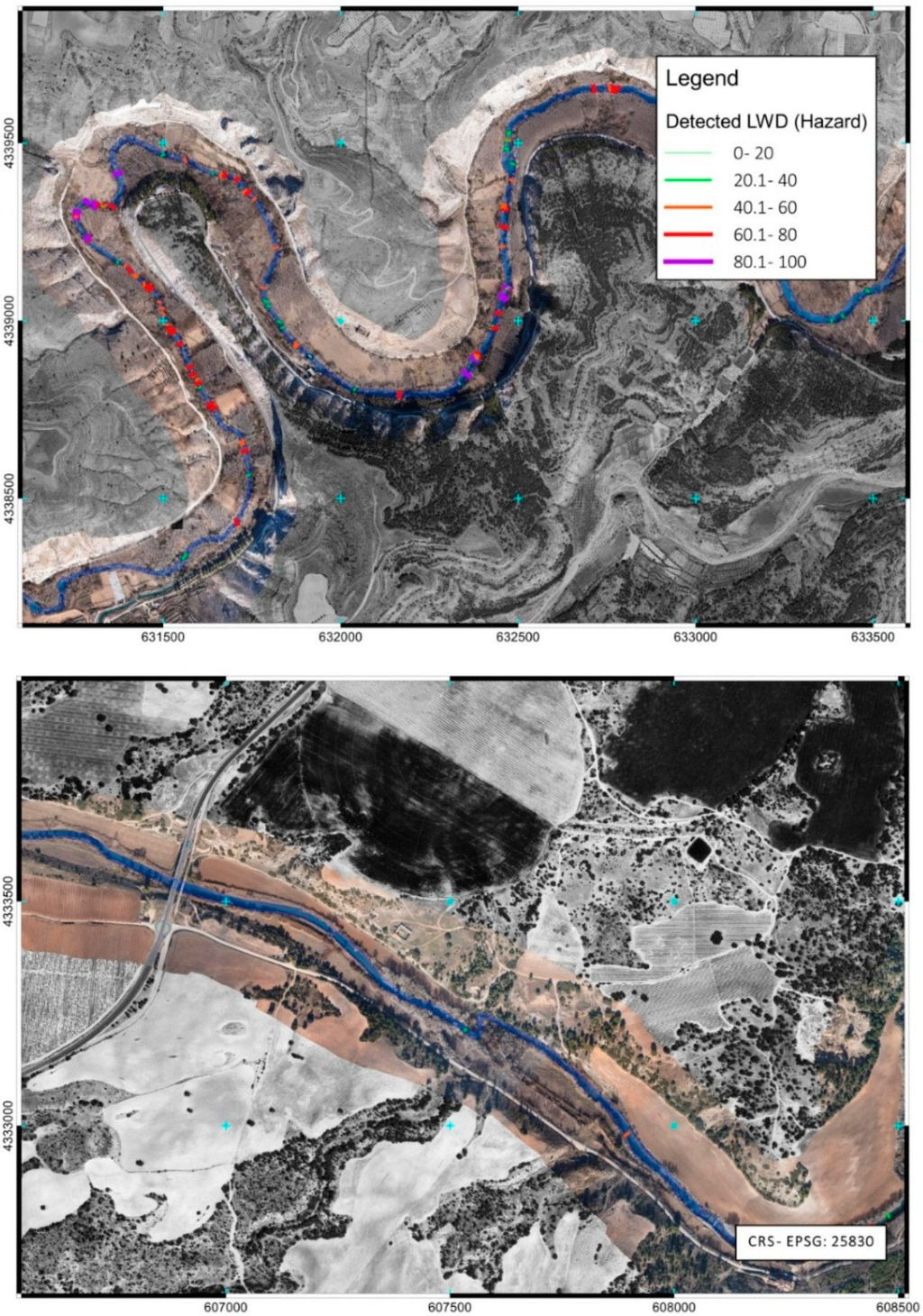
Figure 8.
Two different stretches of the Júcar River where LWD was detected, with high and low density of LWD detected.
Figure 8.
Two different stretches of the Júcar River where LWD was detected, with high and low density of LWD detected.

Once the proposed methodology was applied and the developed FOSSGIS plugin implemented, 927 individuals were detected and digitalized. Figure 9 shows the distribution function of the four parameters that determines the level of risk of the LWD in regards to flooding.
It can be observed that the distribution function of the distance of the barycenter of the LWD to the river axis (Figure 9b) and the number of LWD individuals in the neighboring area (closer to 100 m) (Figure 9d) were very asymmetric, with a tendency toward low values. However, the length of the LWD (Figure 9a) and the percentage that the LWD occupies of the transversal section of the river (Figure 9c) had a more symmetric distribution centered approximately in the average value. The higher weight of the third parameter determined the shape of the distribution function of the level of risk (Figure 10), although a slightly left-asymmetric distribution is also obtained. This information could contribute to allocating the available economic resources in those LWD individuals that actually represented a risk for flooding.
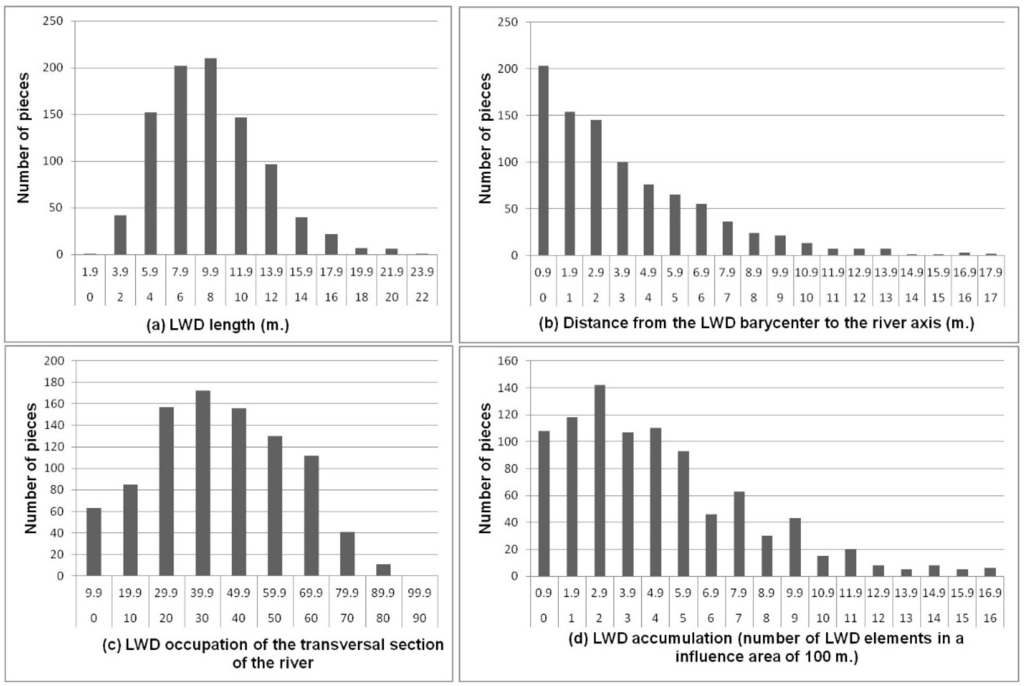
Figure 9.
Histograms of the four parameters that determine the level of risk of the LWD.
Figure 9.
Histograms of the four parameters that determine the level of risk of the LWD.

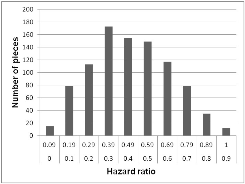
Figure 10.
Histogram of the level of hazard of the detected LWD.
Figure 10.
Histogram of the level of hazard of the detected LWD.
Many other potential applications of the obtained geomatic product were evaluated, such as an improved control of the restricted-use area of the river, development of 3D models of the river floodplain for flooding control, evaluation of the total mass of LWD, and others, which can be utilized in DSS models for river management [44,45,46]. It is also important to evaluate the temporal dynamics of wood in rivers, as well as the pattern of the riparian vegetation on time [47]. The proposed methodology also permits re-visiting the controlled area with a low cost compared with other systems, such as airplanes, and with the capacity of covering a larger area compared with unmanned aerial vehicles. Although it was not the objective of this paper, the proposed technique could be utilized to monitor riparian vegetation with the aim of performing a quantitative evaluation of funded action efficiencies and gaining a detailed understanding of vegetation pattern and dynamics [48].
For the method validation, an LWD removal action was carried out by the Watershed Authority (Figure 11). Concretely, it took place in an area limited by two transversal barriers: Maldonado Bridge and Jorquera weir. This area was selected due to its high hazards ratio, since 109 elements of the 927 identified for the 132 km of the study area were classified in 6.9 km. During the execution of these actions in specific sections, a control was carried out by the technicians to verify the presence of the LWD detected with the proposed methodology. Three different classification results were obtained:
- (a)
- LWD elements identified by the proposed method, the existence of which was verified during the removal action.
- (p)
- New LWD detected during the removal action. This is caused by:
- (1)
- Trees occluded by others trees.
- (2)
- Areas where riparian vegetation covers the whole river (gallery forest).
- (3)
- Occlusions by constructions (bridges, gauging stations, etc.).
- (c)
- LWD elements identified by the proposed method, the existence of which was not possible to verify during the removal action. This is caused by the LWD that had been moved in the interval time between the flight and the action.
The results are summarized in Table 2:
Table 2.
Summary of field verification for LWD classification.
| Field Check | |||
|---|---|---|---|
| Verified | Non-Verified | ||
| Classified | 105 | 4 | |
| Non-Classified | Occlusions by trees | 4 | - |
| Gallery forest occlusion | 2 | - | |
| Occlusions by factory works | 1 | - | |
As a result, the number of LWD was underestimated by 6%. As a methodology limitation, seven LWD elements were not detected due to occlusion in the data acquisition from the airborne platform. The non-verified LWD highlight the relevance of the temporal separation between the flight and the removal.
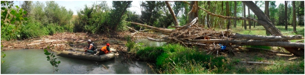
Figure 11.
LWD removal action by the water authorities.
Figure 11.
LWD removal action by the water authorities.

3.4. Economic Analysis
Three different methods were compared with the proposed one: (1) traditional method; (2) navigation method; and (3) conventional photogrammetry. Table 3 shows the total cost of the different methodologies, except the first (traditional method listed in Section 2.7), which was not comparable with the others, because it could not be applied to the 132-km segment of the river, and it was only applied in problematic stretches.
Table 3.
Total cost of the different evaluated methodologies to detect LWD in the 132-km stretch of the Júcar River.
| Methodology | Sub-Tasks | Cost, € | Cost, € |
|---|---|---|---|
| Navigation method | GPS data acquisition | 5560 | 10,945 |
| Boat renting | 1330 | ||
| Boat operator | 3540 | ||
| SIG edition and final report | 515 | ||
| Conventional photogrammetry | GNSS stations measurements | 1350 | 9960 |
| Aircraft planning and flight | 6500 | ||
| Quick orthoimage generation | 700 | ||
| GIS digitization | 400 | ||
| Plugin development for hazard assessment | 1000 | ||
| Proposed methodology | Flight operator (>5 years’ experience) | 600 | 6000 |
| Minitrike renting | 1050 | ||
| Flight insurance and displacement | 150 | ||
| Measurement of the control points | 400 | ||
| Photogrammetric workflow | 2390 | ||
| GIS digitization | 400 | ||
| Plugin development for hazard assessment | 1000 |
The navigation method would be 45.2% more expensive than the proposed method. In addition, with the navigation method, it was not possible to locate the relative position of LWD over the river edge, because the presence of very dense riparian vegetation would hinder the GPS signal reception. An additional disadvantage would be the existence of numerous transverse barriers (40 weirs, dams, etc.) along the river. Furthermore, the decision on the classification of the elements would be performed by the operator on board, who typically does not have the capability to make this decision.
The cost of conventional photogrammetry with regular aircraft would be 39.8% more expensive than the proposed method. In addition, there would be a high uncertainty about the timing of the flight, because it depends on the availability of the company that performs this type of work. Additionally, the flight regulations for a minitrike are more flexible than for aircraft. However, the alternative photogrammetric platforms should also meet some weather requirements of flight, among which is that the wind does not exceed a certain threshold. In the case of the mini-trike, this is recommended as <15 km/h. Although the spatial resolution could be even better than with the proposed methodology, reaching in some cases a GSD value of 8 cm, the riparian vegetation could hide part of the river channel due to the high flight altitude and perspective issues. An alternative aerial platform could be a helicopter, but the hourly cost (1500–2000 €/h) is much higher than a minitrike (300 €/h). Helicopter flight time would be around 3–4 h for higher flight height, but the main inconvenience would be the environmental effect on birdlife, because of noise.
It is worth highlighting that the flexibility of the minitrike during flight permits coping with river sinuosity (Figure 8), while for the UAV and aircraft platforms, this will severely increase the flight time and execution costs.
To compare the traditional method with the proposed methodology, the necessity and cost of removing riparian vegetation was evaluated. In 2007, the traditional methodology was applied to detect LWD along 4 km of the river. Removing riparian vegetation to visually detect LWD in the river channel cost 5245 € (71 openings in the riparian vegetation corresponding with 2737 m2). With the proposed methodology, riparian vegetation was removed only where LWD was detected. In this case, only 370 m2 of riparian vegetation had to be removed, with a total cost of 709 €. In addition, the environmental impact was much lower. Typically, the economic impact of high resolution remote sensing techniques is not evaluated in the literature, but it is a key factor in determining the suitability of these techniques [49].
The main disadvantages of the proposed methodology could be summed up as the weather forecast (maximum wind speed, non-rain conditions, thermal current turbulences) and pilot availability for the platform employed. Regarding the LWD detection, the photogrammetry approaches are affected by the vegetation canopy, so the final number of LWD elements are underestimated (Table 2). The alternative approaches and light equipment that would allow the targeting of LWD on sight could be adequate for small river portions without the presence of barriers (natural or artificial), dense riparian vegetation and gallery forest.
4. Conclusions
This study describes a successful methodology that assists in decision making for sustainable management of river channels by generating a low-cost geomatic product to detect the presence and positioning of large woody debris (LWD) as a non-intrusive method. The results showed that the use of low-cost photogrammetry using economical, conventional, non-metric digital cameras mounted on low-cost aircrafts, together with the use of the developed FOSSGIS and open-source geomatic tools, produced useful geomatic products to detect, classify and manage LWD in rivers. In this case study, the geomatic product was used to successfully detect and classify almost 1000 elements of LWD in a 132-km segment of the Júcar River. The classification of the LWD individuals based on the level of risk indicators contributed to allocating the available economic resources in those LWD individuals that actually represented a risk of flooding. The proposed methodology, compared with conventional photogrammetry or other traditional methods (removing vegetation to visually detect LWD or navigation by boat), led to a cost savings of up to 45%. In the validation carried out, the LWD elements were underestimated due to vegetation canopy occlusion. In addition, this approach led to reduced environmental impact on riparian vegetation. Many other potential applications of the obtained geomatic product are being evaluated, such as 3D modelling of the river channel and the temporal pattern of the riparian vegetation, among others.
Acknowledgments
The authors would like to thank Luis Garijo-Alonso, Departmental Head of the Júcar Watershed Authority, for his valuable collaboration and assistance.
Author Contributions
All authors contributed extensively to the work presented in this paper, except for the plugin for automatic LWD classification using FOSSGIS tools, which was developed entirely by Damian Ortega-Terol.
Conflicts of Interest
The authors declare no conflict of interest.
References
- QGIS. Available online: http://www.qgis.org (accessed on 1 October 2014).
- Jones, T.A.; Daniels, L.D.; Powell, S.R. Abundance and function of large woody debris in small, headwater streams in the Rocky Mountain foothills of Alberta, Canada. River Res. Appl. 2011, 27, 297–311. [Google Scholar] [CrossRef]
- Kail, J. Influence of large woody debris on the morphology of six central European streams. Geomorphology 2003, 51, 207–223. [Google Scholar] [CrossRef]
- Cordova, J.M.; Rosi-Marshall, E.J.; Yamamuro, A.M.; Lamberti, G.A. Quantity, controls and functions of large woody debris in Midwestern USA streams. River Res. Appl. 2007, 23, 21–33. [Google Scholar] [CrossRef]
- Máčka, Z.; Krejčí, L.; Loučková, B.; Peterková, L. A critical review of field techniques employed in the survey of large woody debris in river corridors: A central European perspective. Environ. Monit. Assess. 2011, 181, 291–316. [Google Scholar] [CrossRef] [PubMed]
- Gregory, K.J.; Davis, R.J. Coarse woody debris in stream channels in relation to river channel management in woodland areas. Regul. Rivers Res. Manag. 1992, 7, 117–136. [Google Scholar] [CrossRef]
- Gurnell, A.M.; Gregory, K.J.; Petts, G.E. The role of coarse woody debris in forest aquatic habitats: Implications for management. Aquat. Conserv. Mar. Freshw. Ecosyst. 1995, 5, 143–166. [Google Scholar] [CrossRef]
- Piégay, H.; Gurnell, A.M. Large woody debris and river geomorphological pattern: Examples from SE France and S. England. Geomorphology 1997, 19, 99–116. [Google Scholar] [CrossRef]
- Chin, A.; Laurencio, L.R.; Daniels, M.D.; Wohl, E.; Urban, M.A.; Boyer, K.L.; Butt, A.; Piegay, H.; Gregory, K.J. The significance of perceptions and feedbacks for effectively managing wood in rivers. River Res. Appl. 2014, 30, 98–111. [Google Scholar] [CrossRef]
- Trayler, K. WN9—Water Notes; Water and Rivers Commission: Perth, Western Australia, Australia, 2000. [Google Scholar]
- Anderson, B.G.; Rutherfurd, I.D.; Western, A.W. An analysis of the influence of riparian vegetation on the propagation of flood waves. Environ. Model. Softw. 2006, 21, 1290–1296. [Google Scholar] [CrossRef]
- Schuett-Hames, D.; Plues, A.E.; Ward, J.; Fox, M.; Light, J. TFW Monitoring Program Method Manual for the Large Woody Debris Survey; NW Indian Fisheries Commission, Timber, Fish & Wildlife: Olympia, WA, USA, 1999. [Google Scholar]
- Kise, M.; Zhang, Q. Creating a panoramic field image using multi-spectral stereovision system. Comput. Electron. Agric. 2008, 60, 67–75. [Google Scholar] [CrossRef]
- Herwitz, S.R.; Johnson, L.F.; Dunagan, S.E.; Higgins, R.G.; Sullivan, D.V.; Zheng, J.; Lobitz, B.M.; Leung, J.G.; Gallmeyer, B.A.; Aoyagi, M.; et al. Imaging from an unmanned aerial vehicle: Agricultural surveillance and decision support. Comput. Electron. Agric. 2004, 44, 49–61. [Google Scholar] [CrossRef]
- Dunford, R.; Michel, K.; Gagnage, M.; Piégay, H.; Trémelo, M.L. Potential and constraints of Unmanned Aerial Vehicle technology for the characterization of Mediterranean riparian forest. Int. J. Remote Sens. 2009, 30, 4915–4935. [Google Scholar] [CrossRef]
- Watts, A.; Perry, J.H.; Smith, S.E.; Burgess, M.A.; Wilkinson, B.E.; Szantoi, Z.; Ifju, P.G.; Percival, H.F. Small unmanned aircraft systems for low-altitude aerial surveys. J. Wildl. Manag. 2010, 74, 1614–1619. [Google Scholar] [CrossRef]
- Marcus, W.A.; Legleiter, C.J.; Aspinall, R.J.; Boardman, J.W.; Crabtree, R.L. High spatial resolution hyperspectral mapping of in-stream habitats, depths, and woody debris in mountain streams. Geomorphology 2003, 55, 363–380. [Google Scholar] [CrossRef]
- Lejot, J.; Delacourt, C.; Piégay, H.; Fournier, T.; Trémélo, M.L.; Allemand, P. Very high spatial resolution imagery for channel bathymetry and topography from an unmanned mapping controlled platform. Earth Surf. Process. Landf. 2007, 32, 1705–1725. [Google Scholar] [CrossRef]
- Aber, J.S.; Marzolff, I.; Ries, J. Small-Format Aerial Photography: Principles, Techniques and Applications; Elsevier: Amsterdam, The Netherlands, 2010. [Google Scholar]
- Olsen, R.C. Remote Sensing from Air and Space; SPIE Press: Bellingham, WA, USA, 2007; Volume 162. [Google Scholar]
- Szantoi, Z.; Malone, S.; Escobedo, F.; Misas, O.; Smith, S.; Dewitt, B. A tool for rapid post-hurricane urban tree debris estimates using high resolution aerial imagery. Int. J. Appl. Earth Observ. Geoinf. 2012, 18, 548–556. [Google Scholar] [CrossRef]
- Del Pozo, S.; Rodríguez-Gonzálvez, P.; Hernández-López, D.; Felipe-García, B. Vicarious radiometric calibration of a multispectral camera on board an unmanned aerial system. Remote Sens. 2014, 6, 1918–1937. [Google Scholar] [CrossRef]
- GeoEye. Available online: http://www.digitalglobe.com/sites/default/files/DG_GeoEye1_Update2014_DS.pdf (accessed on 14 July 2014).
- Kraus, K. Photogrammetry: Geometry from Images and Laser Scans; Walter De Gruyter: Berlin, Germany, 2007. [Google Scholar]
- Kemper, G. New airborne sensors and platforms for solving specific tasks in remote sensing. Int. Arch. Photogramm. Remote Sens. Spat. Inf. Sci. 2012, XXXIX-B5, 351–356. [Google Scholar]
- Li, C.; Li, H.; Kemper, G. Monitoring urban development of small Chinese cities using innovative aerial surveying technologies. Int. Arch. Photogramm. Remote Sens. Spat. Inf. Sci. 2008, XXXVII, 1667–1674. [Google Scholar]
- Küng, O.; Strecha, C.; Beyeler, A.; Zufferey, J.C.; Floreano, D.; Fua, P.; Gervaix, F. The accuracy of automatic photogrammetric techniques on ultra-light UAV imagery. In Proceedings of the International Conference on Unmanned Aerial Vehicle in Geomatics (UAV-g), Zurich, Switzerland, 14–16 September 2011; pp. 14–16.
- Vallet, J.; Panissod, F.; Strecha, C.; Tracol, M. Photogrammetric performance of an ultra light weight swinglet “UAV”. In Proceedings of the International Conference on Unmanned Aerial Vehicle in Geomatics (UAV-g), Zurich, Switzerland, 14–16 September 2011; pp. 253–258.
- Smith, S.; Szantoi, Z.; Perry, J.; Percival, F.; Evers, B. Design considerations for remote sensing payloads on inexpensive unmanned autonomous aerial vehicles. Surv. Land Inf. Sci. 2010, 70, 131–137. [Google Scholar]
- CNIG. Available online: http://centrodedescargas.cnig.es/CentroDescargas (accessed on 14 July 2014).
- DIY Drones. Available online: http://diydrones.com/profiles/blogs/arduimu-quadcopter-part-ii (accessed on 14 July 2014).
- Premerlani, W.; Bizard, P. Direction Cosine Matrix IMU: Theory. Available online: http://gentlenav.googlecode.com/files/DCMDraft2.pdf (accessed on 14 July 2014).
- NavCen. Global Positioning System Standard Positioning Service Performance Standard, 4th ed.; US Department of Defense: Position, Navigation, and Timing Executive Committee: Washington, DC, USA, 2008. [Google Scholar]
- Takasu, T. RTKLIB: Open source program package for RTK-GPS. In Proceedings of the FOSS4G 2009, Tokyo, Japan, 1–2 November 2009.
- Sauerbier, M.; Siegrist, E.; Eisenbeiss, H.; Demir, N. The practical application of UAV-based photogrammetry under economic aspects. In Proceedings of the International Conference on Unmanned Aerial Vehicle in Geomatics (UAV-g), Zurich, Switzerland, 14–16 September 2011; pp. 45–50.
- El-Rabbany, A. Introduction to GPS: The Global Positioning System; Artech House: Boston, MA, USA, 2002. [Google Scholar]
- Pierrot-Deseilligny, M.; Clery, I. Apero, an open source bundle adjusment software for automatic calibration and orientation of set of images. Int. Arch. Photogramm. Remote Sens. Spat. Inf. Sci. 2011, XXXVIII-5/W16, 269–276. [Google Scholar]
- Lowe, D.G. Distinctive image features from scale-invariant keypoints. Int. J. Comput. Vis. 2004, 60, 91–110. [Google Scholar] [CrossRef]
- Hirschmuller, H. Stereo processing by semiglobal matching and mutual information. IEEE Trans. Pattern Anal. Mach. Intell. 2008, 30, 328–341. [Google Scholar] [CrossRef] [PubMed]
- Chen, D.; Shams, S.; Carmona-Moreno, C.; Leone, A. Assessment of open source GIS software for water resources management in developing countries. J. Hydro-Environ. Res. 2010, 4, 253–264. [Google Scholar] [CrossRef]
- Teodoro, A.C.; Duarte, L. Forest fire risk maps: A GIS open source application—A case study in Norwest of Portugal. Int. J. Geogr. Inf. Sci. 2012, 27, 699–720. [Google Scholar] [CrossRef]
- Gaia-SINS. Available online: http://www.gaia-gis.it/gaia-sins/ (accessed on 14 July 2014).
- Wohl, E.; Cenderelli, D.A.; Dwire, K.A.; Ryan-Burkett, S.E.; Young, M.K.; Fausch, K.D. Large in-stream wood studies: A call for common metrics. Earth Surf. Process. Landf. 2010, 35, 618–625. [Google Scholar]
- Gichamo, T.Z.; Popescu, I.; Jonoski, A.; Solomatine, D. River cross-section extraction from the ASTER global DEM for flood modeling. Environ. Model. Softw. 2012, 31, 37–46. [Google Scholar] [CrossRef]
- Lacroix, M.P.; Martz, L.W.; Kite, G.W.; Garbrecht, J. Using digital terrain analysis modeling techniques for the parameterization of a hydrologic model. Environ. Model. Softw. 2002, 17, 125–134. [Google Scholar] [CrossRef]
- Lautenbach, S.; Jürgen, B.; Graf, N.; Seppelt, R.; Matthies, M. Scenario analysis and management options for sustainable river basin management: Application of the Elbe DSS. Environ. Model. Softw. 2009, 24, 26–43. [Google Scholar] [CrossRef]
- MacVicar, B.J.; Piégay, H.; Henderson, A.; Comiti, F.; Oberlin, C.; Pecorari, E. Quantifying the temporal dynamics of wood in large rivers: Field trials of wood surveying, dating, tracking, and monitoring techniques. Earth Surf. Process. Landf. 2009, 34, 2031–2046. [Google Scholar] [CrossRef]
- Dufour, S.; Bernez, I.; Betbeder, J.; Corgne, S.; Hubert-Moy, L.; Nabucet, J.; Rapinel, S.; Sawtschuk, J.; Trollé, C. Monitoring restored riparian vegetation: How can recent developments in remote sensing sciences help? Knowl. Manag. Aquat. Ecosyst. 2013. [Google Scholar] [CrossRef]
- Zhang, C.; Kovacs, J. The application of small unmanned aerial systems for precision agriculture: A review. Precis. Agric. 2012, 13, 693–712. [Google Scholar] [CrossRef]
© 2014 by the authors; licensee MDPI, Basel, Switzerland. This article is an open access article distributed under the terms and conditions of the Creative Commons Attribution license (http://creativecommons.org/licenses/by/4.0/).