Analysis of MERIS Reflectance Algorithms for Estimating Chlorophyll-a Concentration in a Brazilian Reservoir

Abstract

Chlorophyll-a (chl-a) is a central water quality parameter that has been estimated through remote sensing bio-optical models. This work evaluated the performance of three well established reflectance based bio-optical algorithms to retrieve chl-a from in situ hyperspectral remote sensing reflectance datasets collected during three field campaigns in the Funil reservoir (Rio de Janeiro, Brazil). A Monte Carlo simulation was applied for all the algorithms to achieve the best calibration. The Normalized Difference Chlorophyll Index (NDCI) got the lowest error (17.85%). The in situ hyperspectral dataset was used to simulate the Ocean Land Color Instrument (OLCI) spectral bands by applying its spectral response function. Therefore, we evaluated its applicability to monitor water quality in tropical turbid inland waters using algorithms developed for MEdium Resolution Imaging Spectrometer (MERIS) data. The application of OLCI simulated spectral bands to the algorithms generated results similar to the in situ hyperspectral: an error of 17.64% was found for NDCI. Thus, OLCI data will be suitable for inland water quality monitoring using MERIS reflectance based bio-optical algorithms.

1. Introduction

Water resources managers are committed to assuring the availability of water in adequate quantity and quality for its multiple mankind uses. They are also committed to maintaining the recreational and ecological amenities of the environment [1]. For that, it is essential to monitor the quality of inland waters, mainly the water supply aquatic systems. One of the most important aspects for water quality management is the level of phytoplankton activity within the water body [2], which is usually represented by phytoplankton biomass.

Phytoplankton is also frequently used as a bioindicator of water quality. This is possiblly because it is one of the water quality parameters that responds most quickly to environmental changes [3]. Its response can be monitored using remotely sensed data through the observations of the optical changes in the reflected light at specific wavelengths. Therefore, these changes can be related to the concentration of phytoplankton’s main and major pigment: Chlorophyll-a (chl-a). This ubiquitous phytoplankton pigment exhibits a unique spectral absorption signature with two marked peaks: one in the blue region of the spectrum (~433 nm); and another one in the red region of the spectrum (~686 nm) [4,5,6]. Its main reflectance peak is in the green channel, around 550 nm [5,7], with a secondary peak around 715 nm, associated with high scattering by the phytoplankton cells [5]. Because of these specific signatures, the estimation of chl-a concentration by remote sensing has been possible [8,9,10,11,12]. Furthermore, it can be an effective tool for environmental managers since it can provide synoptic and repetitive quantitative information about the aquatic systems.

A wide range of algorithms have been developed for retrieving chl-a [3,8,9,10,11,12,13]. Two comprehensive reviews of algorithms for retrieving a variety of parameters from remote sensing including the estimation of chl-a can be found in Matthews [14] and Odermatt et al. [15]. The success of these algorithms depends on the biogeochemical characteristics of the water body. In marine optics, much progress has been made in the retrieval of this pigment from blue-to-green ratios of remote sensing reflectance [16,17,18]. The ratio of these two spectral channels worked well in ocean waters since phytoplankton is usually their predominant constituent and the concentrations of suspended solids (SS) and dissolved organic matter (DOM) correlate with it. Problems have arisen for coastal and inland waters where SS and DOM have higher values and their concentrations do not always correlate with chl-a. Thus, all constituents that are present in these waters affect their optical properties.

The overlapping and uncorrelated absorptions by DOM and non-algal particles (NAP) in the blue region of the spectrum, renders the blue-to-green ratio inaccurate for estimating chl-a concentration in waters where these components are not correlated to phytoplankton [18,19]. Hence, for retrieving chl-a, reflectance based algorithms focus on the spectral properties of chl-a in the red and near infrared (NIR) channels.

Bio-optical models are parameterized to fit satellite bandwidth so they can be repetitively used for retrieving biogeochemical concentration over the world. One of the satellite sensor most used for aquatic studies was the MEdium Resolution Imaging Spectrometer (MERIS). MERIS was a sensor whose spectral bands were positioned aiming to capture the spectral features of the different components in the water [20]. In 2012, 10 years after its launch, this sensor stopped sending data to Earth, but the continuity of MERIS measurement capability is particularly important for water bodies (including water quality) and climate monitoring applications [21]. For this purpose, its successor will be send into space onboard of the two Sentinel 3 satellites which will image Earth in constellation: the Ocean and Land Color Instrument (OLCI). However, new sensors have to be tested using in situ radiometric measurements. Therefore, the main goal of this study was to evaluate the use of MERIS reflectance based chl-a algorithms using in situ hyperspectral data and OLCI simulate bands.

2. Material and Methods

2.1. Study Area

The study area was the Funil Hydroelectric Reservoir (44º55′W; 21º05′S, see Figure 1) located in Itatiaia, Rio de Janeiro state, Brazil. Formed by the damming of Paraíba do Sul River in its medium course, it has a flooded area of 40 km² with maximum depth of 70 m and average depth of 20 m [22]. The catch basin covers almost entirely the São Paulo portion of the Paraíba Valley which is one of the most industrialized axes of Brazil with intense economic activity. Thus, the number of large industries with high pollution potential is significant [23].

Figure 1. (A) Location of Funil Hydroelectric Reservoir. Sampling points from: (B) May 2012, (C) September 2012; and (D) April 2013. Color Composite TM-Landsat5 R3G2B1. Orbit/Point: 218/76. Date of Passage: 5 September 2011.

Figure 1. (A) Location of Funil Hydroelectric Reservoir. Sampling points from: (B) May 2012, (C) September 2012; and (D) April 2013. Color Composite TM-Landsat5 R3G2B1. Orbit/Point: 218/76. Date of Passage: 5 September 2011.

Industrial development and urban expansion contributed to enhance degradation which lead to a mischaracterization of basin environmental conditions. Waters drained from these industrial areas are the main source of water pollution in Funil. Domestic sewage, industrial effluents and sand extraction in the river contribute to increase turbidity and siltation on the reservoir. Therefore, these factors collaborate to the loss of water quality in this water body [24].

For the regions downstream the reservoir, Funil dam acts as a barrier to the São Paulo State pollution. It accumulates nutrients; toxic substances; and sediment drained by Paraíba do Sul River. As a result, several studies have already demonstrated the constant presence of high values of phytoplankton biomass [25,26,27,28]. It constantly undergoes high primary productivity with reduced transparency and frequent occurrences of algal blooms that reduce the dissolved oxygen, which can lead to fish mortality.

2.2. Datasets

Datasets were collected during three field campaigns held in 20–22 May 2012, 2–4 September 2012, and 2–5 April 2013. In the May and April campaigns the hydrological period was high-water, which occurs right after the rainy season (austral summer). In September, the reservoir was operating at low capacity, after a long period of drought (austral winter), with a lowering of the water level of more than 10 meters. Sampling points were distributed homogeneously along the reservoir for the May and September campaigns (Figure 1B,C). For the April campaign (Figure 1D) we only collected the data from the river inlet. In all sampling points we collected water samples for limnological analysis at the same time we collected the radiometric data.

2.2.1. Remote Sensing Reflectance

Two submersible radiometers (TriOS RAMSES-Oldenburg, Germany) were used for in situ radiometric measurements during the three field campaigns. Spectral measurements of upwelling radiance (L_u) just below the air-water interface; and downwelling plane irradiance (E_d) right above the air-water interface; were collected using RAMSES-ARC-UV/VIS and RAMSES-ACC-UV/VIS, respectively.

These instruments were mounted on a frame in which their optical axes were aligned parallel to each other. Depth and inclination measurements were acquired by a pressure and tilt sensor integrated into the RAMSES-ACC-UV/VIS. Each sensor has 190 useable channels from 320 nm to 950 nm with the spectral sampling interval of 3.3 nm and 0.3 nm of accuracy [29].

The radiometric measurements were collected at a distance of 1.5 meter from the boat, reducing any shading effects. All measurements were made simultaneously following the acquisition protocol from Hooker [30] and Mobley [31]. The Remote Sensing Reflectance (R_RS) above the water surface was then calculated based on Mobley [31] as described in Equation 1.

$$R_{RS}=\frac{t\bullet L_u}{n^2\bullet E_d}$$

(1)

where, t is the transmittance at the air-water interface (0.98); and n is the refractive index of water (1.34).

We used Mobley’s [31] equation to achieve R_RS because the underwater measurement of L_u is not influenced by sky reflection or sun glint, but it can only be performed at single stations and has to be extrapolated to the water surface [32] using equations and in the conditions stated by Mobley [31].

For each sampling point, ten measurements of both irradiance and radiance were acquired and the average spectrum was calculated to achieve R_RS. The R_RS spectra were resampled to 1 nm using linear interpolation. A synthetic dataset was created by applying the OLCI spectral response function to the R_RS spectra.

2.2.2. Chl-a

Water samples for chl-a determination were collected at all sampling stations on the surface of Funil Hydroelectric Reservoir (about 10 cm deep) at the same time the radiometric data was being acquired. These samples were kept on ice until the arrival on land where the filtering procedure with 0.7 mm Whatman GF/F was conducted. The filters were then frozen until they were delivered to the laboratory for the extraction of the chl-a pigment using acetone and measuring its absorbance in a Varian Cary 50 Conc UV-VIS spectrophotometer (Agilent Technologies, Santa Clara, CA, USA) following Nush [33] method. Some of the samples were collected at duplicates and the chl-a concentrations were calculated from the absorbance data using the equations from Lorenzen [34].

Table 1 and Figure 2 show the summary of chl-a data for the three campaigns. The datasets collected are representative for a large range of chl-a concentrations. The analysis of the standard deviation in Table 1 shows low values for May and April with higher value for September. We also observed the discrepancy between Average and Median values. In May and April they are cohesive, but in September they are distinct, which can be explained by the small number of high concentration values of chl-a in September. Those values influence the average, making it larger than the median as shown in Figure 2.

Table 1. Summary statistics for chl-a (concentrations in µg∙L⁻¹) at each campaign.

	Maximum	Minimum	Range	Average	Median	Standard Deviation
May 2012	32.96	2.33	30.63	8.59	4.88	7.81
September 2012	306.03	4.37	301.67	67.08	14.82	90.80
April 2013	52.78	4.92	47.86	19.49	12.89	15.28

Table 1. Summary statistics for chl-a (concentrations in µg∙L⁻¹) at each campaign.

	Maximum	Minimum	Range	Average	Median	Standard Deviation
May 2012	32.96	2.33	30.63	8.59	4.88	7.81
September 2012	306.03	4.37	301.67	67.08	14.82	90.80
April 2013	52.78	4.92	47.86	19.49	12.89	15.28

Figure 2. Box-plots with the summary statistics for chl-a (concentrations in µg∙L⁻¹) at each campaign.

Figure 2. Box-plots with the summary statistics for chl-a (concentrations in µg∙L⁻¹) at each campaign.

2.3. Chl-a MERIS Bio-Optical Models

Three bio-optical models were evaluated in this study to estimate the chl-a concentration based on the RED-NIR relationship. The chosen models were already parameterized for inland waters and fitted to MERIS spectral bands. The use of the RED-NIR relationship is a strategy to reduce the interference in the signal of other components in the water column [12,35], although variations of specific absorption coefficient of chl-a can be a limitation [19]. The analysis of these specific models parameterized for MERIS addresses their applicability to the OLCI sensor. Table 2 summarizes the models.

Table 2. Summary of R_RS based bio-optical models to retrieve chl-a concentration. Where: Chl-a is the chlorophyll-a concentration; and R_RS is the Remote Sensing Reflectance obtained by Equation (1) at specific wavelengths.

Abbreviation	Reference	Model
2BDA	19	$Chl-a\approx \frac{R_{RS}(709)}{R_{RS}(665)}$
3BDA	36	$Chl-a\approx (R_{RS}{\left(665\right)}^{-1}-R_{RS}{\left(709\right)}^{-1})\bullet R_{RS}(753)$
NDCI	12	$Chl-a\approx \frac{R_{RS}(709)-R_{RS}(665)}{R_{RS}\left(709\right)+R_{RS}(665)}$

Table 2. Summary of R_RS based bio-optical models to retrieve chl-a concentration. Where: Chl-a is the chlorophyll-a concentration; and R_RS is the Remote Sensing Reflectance obtained by Equation (1) at specific wavelengths.

Abbreviation	Reference	Model
2BDA	19	$Chl-a\approx \frac{R_{RS}(709)}{R_{RS}(665)}$
3BDA	36	$Chl-a\approx (R_{RS}{\left(665\right)}^{-1}-R_{RS}{\left(709\right)}^{-1})\bullet R_{RS}(753)$
NDCI	12	$Chl-a\approx \frac{R_{RS}(709)-R_{RS}(665)}{R_{RS}\left(709\right)+R_{RS}(665)}$

Gitelson et al. [36] proposed an algorithm to retrieve chl-a in higher plant leaves. Later, Dall’Olmo and Gitelson [19] applied this model (3BDA) and presented its special case (2BDA) for turbid productive waters. Gitelson et al. [8] estimated chl-a concentration using these two models with datasets collected from lakes and reservoirs in Nebraska (sandpit lakes and reservoirs in Eastern Nebraska), Iowa (Lake Okoboji), Minnesota (Lake Minnetonka) and Maryland (Choptank River–Chesapeake Bay). They found a chl-a range from 1.2 to 236 µg·L⁻¹ and found a R² equal 0.94 and 0.93 for 3BDA and 2BDA, respectively.

Mishra and Mishra [12] based on the Normalized Difference Vegetation Index (NDVI) proposed the Normalized Difference Chlorophyll Index (NDCI) to predict chl-a concentration from MERIS images in estuarine and coastal turbid productive waters. Their results indicate that the NDCI was successful in predicting chl-a concentration in the range from 0.9 to 28.1 µg∙L⁻¹ with R² of 0.9. They applied this model to several study sites: Chesapeake Bay, Delaware Bay, Mobile Bay, and the Mississippi River delta region in the northern Gulf of Mexico, USA.

2.4. Calibration and Validation

The radiometric and limnological data acquired in all field campaigns were merged in unique dataset and used to calibrate the algorithms listed in Table 2. We joined all field data from the three campaigns, separated the extreme data, split the remaining data into quartiles and used three samples of each quartile for validation. As a result, we ended up with 28 samples for calibration and 12 for validation.

We considered extreme data the chl-a concentrations higher than 20 µg∙L⁻¹. The use of this limit is justified because the dataset was composed of a major number of data below this value (40 samples) and the other samples were mainly concentrated above 100 µg∙L⁻¹. We split the extreme samples (12 values) from the dataset, as it is not representative for the normal behavior of the reservoir. These samples were obtained during bloom condition, with optical characteristics of phytoplankton dominance [37], which is not the natural behavior for most of the time of the year.

To assure this difference between bloom and non-bloom conditions, we also calibrated and validated all models with all data available. Eight samples with extreme values were included in calibration, leaving the other four for validation. We then had 36 samples for calibration and 16 for validation. The comparison of these results with the calibration using only data with chl-a values under 20 µg∙L⁻¹ was conducted to enhance the need to split the dataset.

To conduct models calibration, we used a Monte Carlo simulation (Figure 3): eight samples were randomly selected and used to calibrate the algorithms with a linear trend between model values and chl-a concentrations. This process was repeated 100,000 times. The resulting values of slope, intercept and determination coefficient (R²) were recorded for each iteration.

Figure 3. Scheme of Monte Carlo simulation to calibrate the models.

Figure 3. Scheme of Monte Carlo simulation to calibrate the models.

The R² histogram was a decision tool to find the equations which had this parameter in its most frequent range. Within this range of R², we plotted the corresponding slope versus intercept of the equations and determined their mode and standard deviations. We selected only the equations that had both slope and intercept in a range based on their mode (mode ± standard deviation). From this group, we selected the equations that had the best R² and validated them using the 12 validation samples. The equation with the lower error estimator was selected as the best. Figure 4 shows a summary scheme of this calibration/validation process.

Figure 4. Calibration/validation scheme.

Figure 4. Calibration/validation scheme.

The error estimators used in this study were: Bias; Root Mean Square Error (RMSE); and Normalized Root Mean Square Error in percentage (NRMSE%). They were calculated according to Table 3. The error estimator used to choose the best equation was NRMSE%. We also generated scatterplots between estimated and measured chl-a concentration to see how close to 1:1 these models are capable to estimate.

Table 3. Summary of the error estimators used. Where: y_i and x_i are the predicted and the measured chl-a concentration respectively in each i sample.

$$Bias=\frac{1}{n}{\displaystyle \sum }_{i=1}^n(y_i-x_i)$$	$RMSE=\sqrt{MSE}$
$$MSE=\frac{1}{n}{\displaystyle \sum }_{i=1}^n{(y_i-x_i)}^2$$	$$NRMSE\%=\frac{RMSE}{∆Chl-a}\bullet 100$$

Table 3. Summary of the error estimators used. Where: y_i and x_i are the predicted and the measured chl-a concentration respectively in each i sample.

$$Bias=\frac{1}{n}{\displaystyle \sum }_{i=1}^n(y_i-x_i)$$	$RMSE=\sqrt{MSE}$
$$MSE=\frac{1}{n}{\displaystyle \sum }_{i=1}^n{(y_i-x_i)}^2$$	$$NRMSE\%=\frac{RMSE}{∆Chl-a}\bullet 100$$

2.5. OLCI Simulated Bands

R_RS hyperspectral dataset was applied to OLCI response function resampled to 1 nm spectral resolution. Each wavelength of R_RS data was multiplied by its response and the results were added and an average response was obtained for each band. The goal was to simulate an approximation of OLCI’ spectral bands and then apply MERIS bio-optical model on them to retrieve chl-a concentration. With OLCI simulated data we performed the calibration/validation using the same processes and models applied to the in situ hyperspectral dataset with chl-a concentration values below 20 µg∙L⁻¹.

3. Results and Discussion

3.1. Remote Sensing Reflectance Behavior

Figure 5 shows all R_RS data from field campaigns. It can be noted a substantial reflectance peak around 550 nm, which can be attributed to phytoplankton spectral behavior. The spectral troughs near 620 nm and around 685 nm appear due to phycocyanin strong absorption (representative cyanobacterial pigment) and chl-a, respectively [19,38]. The R_RS feature at the beginning of the near infrared region of the spectrum (700 nm) is also recorded shifting to longer wavelengths with the increase in chl-a concentration following the results of Gitelson [5].

Figure 5. R_RS spectra from Funil reservoir in: (A) May 2012; (B) September 2012 and (C) April 2013.

Figure 5. R_RS spectra from Funil reservoir in: (A) May 2012; (B) September 2012 and (C) April 2013.

3.2. Bio-Optical Models

The models listed in Table 2 were evaluated in the following sections for three conditions: in situ hyperspectral data with chl-a bellow 20 µg∙L⁻¹; all in situ hyperspectral data with no chl-a concentration limit; and OLCI simulated data with chl-a bellow 20 µg∙L⁻¹.

3.2.1. Calibration and Validation of the Hyperespectral Data with chl-a Concentration bellow 20 µg∙L⁻¹

Table 4 shows the results from Monte Carlo analysis. It is clear that the only negative value of the intercept was found for 2BDA. A negative value in the intercept represents the case when there is no chl-a in the water. In this case, the model would produce a value because of the interference of other constituents. On the other hand, a positive intercept means that, at a given concentration of chl-a, the models would have no response, which could mean that the spectral signatures are masked or the model have a limit concentration below what it does not respond. This is not a response expected for a chl-a model.

Table 4. Coefficients derived from model calibrations applied to samples with chl-a concentration bellow 20 µg∙L⁻¹. Hyperspectral data.

	Slope	Intercept	R²
2BDA	41.8	−15.0	0.90
3BDA	581.1	25.5	0.90
NDCI	54.0	23.8	0.90

Table 4. Coefficients derived from model calibrations applied to samples with chl-a concentration bellow 20 µg∙L⁻¹. Hyperspectral data.

	Slope	Intercept	R²
2BDA	41.8	−15.0	0.90
3BDA	581.1	25.5	0.90
NDCI	54.0	23.8	0.90

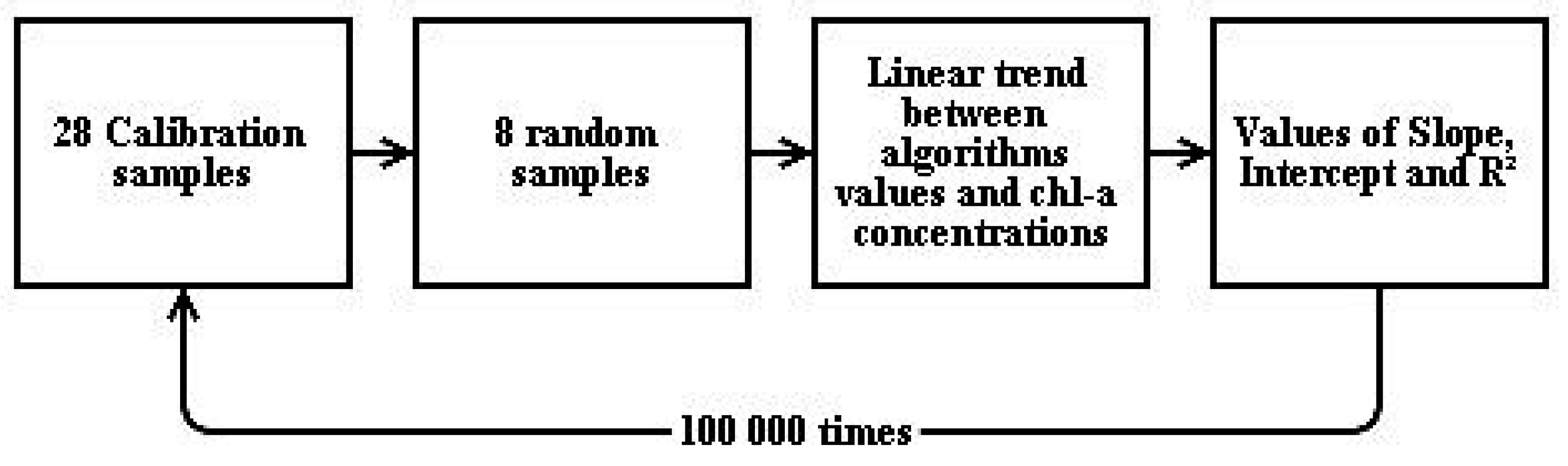
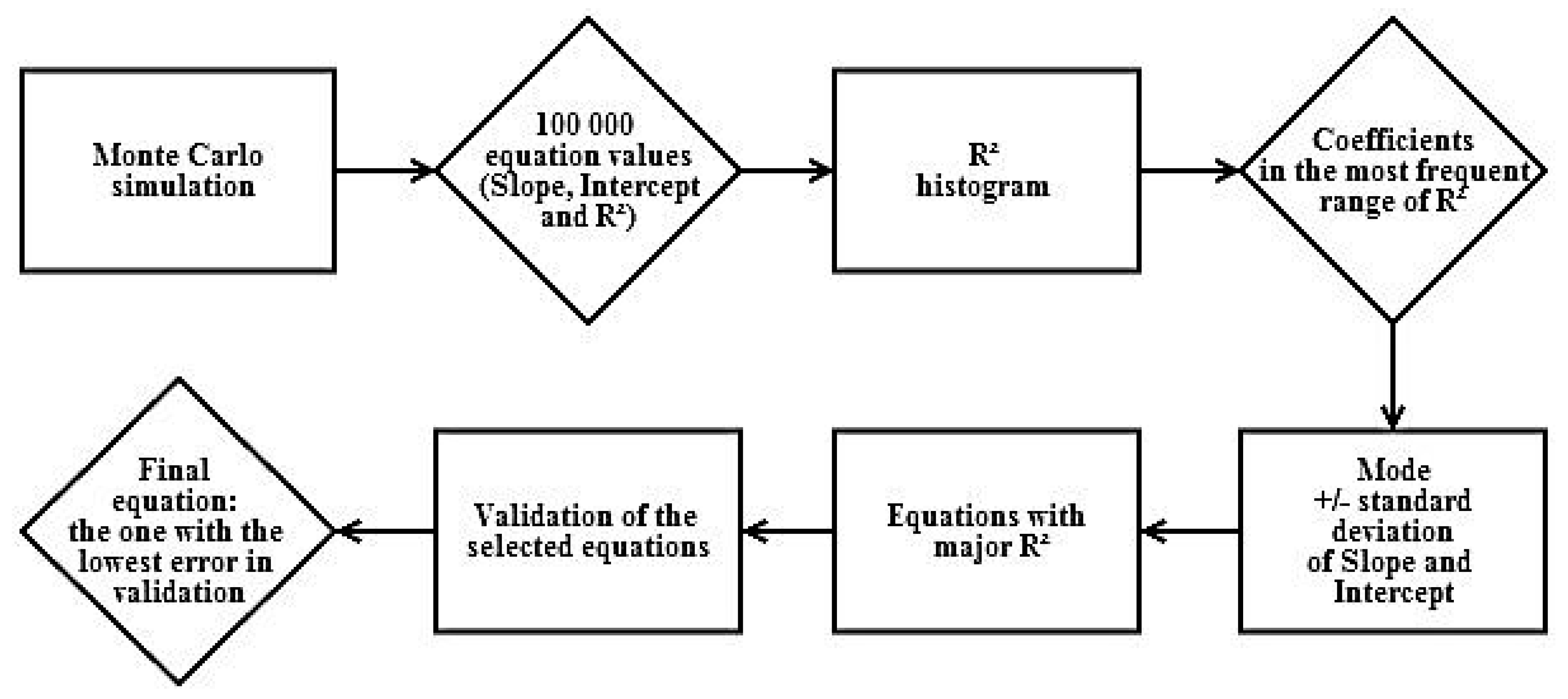
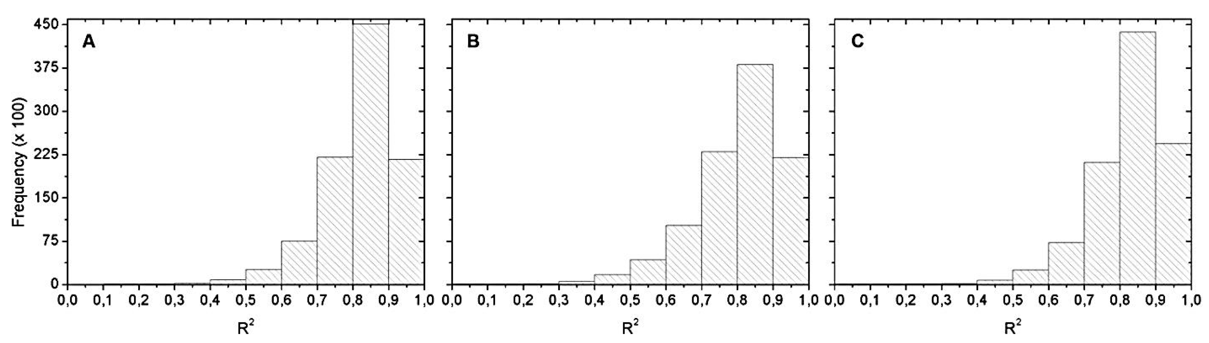
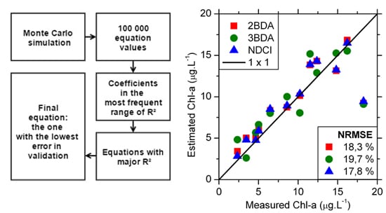
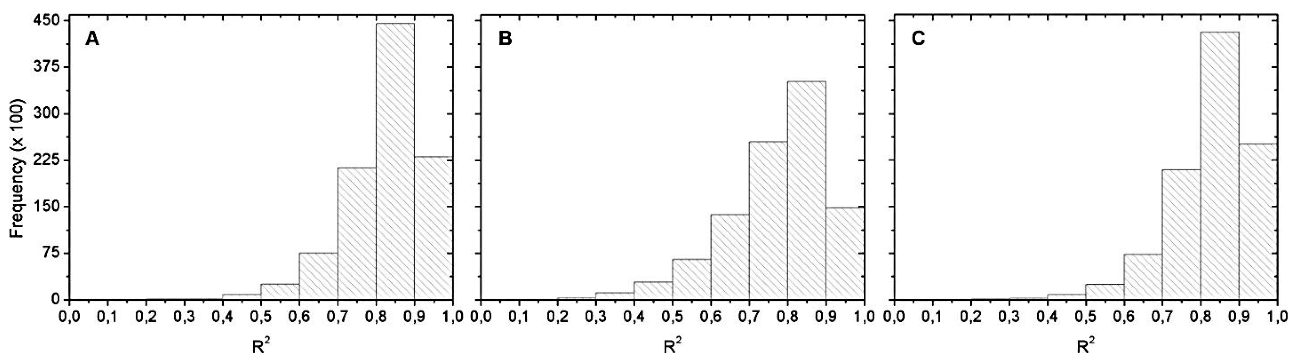
Figure 6 shows the R² histograms from Monte Carlo simulation. The most frequent R² range was between 0.8 and 0.9. Within this range, we chose the best equation of the validation with the maximum R². That is why Table 4 only exhibits R² equals 0.9.

Figure 6. Histograms of the R² distribution for: (A) May 2012; (B) September 2012; and (C) April 2013. Hyperspectral data with chl-a values below 20 µg∙L⁻¹.

Figure 6. Histograms of the R² distribution for: (A) May 2012; (B) September 2012; and (C) April 2013. Hyperspectral data with chl-a values below 20 µg∙L⁻¹.

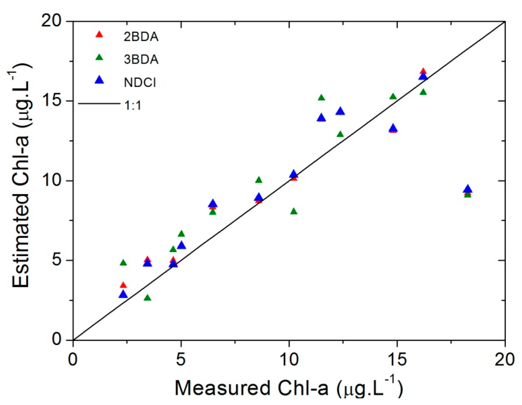
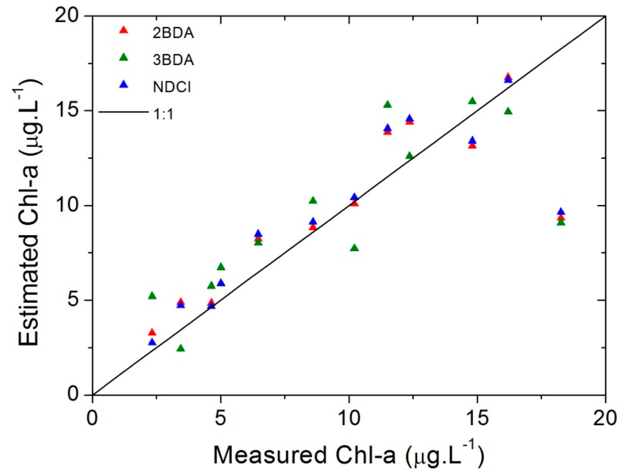
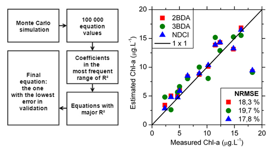
Table 5 shows the error analysis. The lowest errors estimators were achieved with NDCI, with NRMSE% of 17.85%. It is observed from Table 5 and the scatterplot on Figure 7 that NDCI and 2BDA had the best performance. In Figure 7 these are the models that come closer to 1:1 line. Even so, all models diverge from 1:1 line as the chl-a concentration increase to 20 µg∙L⁻¹. This indicates that the parameterization found for these models can only be applied to restricted ranges of chl-a concentrations. Besides that, based on the p value showed in Table 5 obtained by t test, no significant difference between the estimated and the measured chl-a concentration was found for all algorithms for a significance level of 5%.

Table 5. Summary results for validation process using in situ hyperspectral data with chl-a values below 20 µg∙L⁻¹.

	Bias (µg∙L−1)	RMSE (µg∙L−1)	NRMSE%	p Value
2BDA	0.01	2.92	18.32	0.987
3BDA	−0.01	3.14	19.68	0.993
NDCI	−0.03	2.84	17.85	0.970

Table 5. Summary results for validation process using in situ hyperspectral data with chl-a values below 20 µg∙L⁻¹.

	Bias (µg∙L−1)	RMSE (µg∙L−1)	NRMSE%	p Value
2BDA	0.01	2.92	18.32	0.987
3BDA	−0.01	3.14	19.68	0.993
NDCI	−0.03	2.84	17.85	0.970

Figure 7. Scatterplots of the Measured vs. Estimated chl-a for each model using in situ hyperspectral data with chl-a values below 20 µg∙L⁻¹.

Figure 7. Scatterplots of the Measured vs. Estimated chl-a for each model using in situ hyperspectral data with chl-a values below 20 µg∙L⁻¹.

3.2.2. Calibration of All in situ Hyperspectral Data

All samples were calibrated/validated without restraining the chl-a concentration. The results in Table 6 are for calibration and they aren’t conclusive without analyzing the error estimators showed in Table 7. Figure 8 show the R² histograms obtained. The most frequent R² range was between 0.8 and 0.9.

Table 6. Coefficients derived from calibration applied to all in situ hyperspectral data.

	Slope	Intercept	R2
2BDA	47.3	−17.9	0.9
3BDA	714.3	28.9	0.9
NDCI	67.6	28.0	0.9

Table 6. Coefficients derived from calibration applied to all in situ hyperspectral data.

	Slope	Intercept	R2
2BDA	47.3	−17.9	0.9
3BDA	714.3	28.9	0.9
NDCI	67.6	28.0	0.9

Table 7. Summary results for validation process applied to all samples using the hyperspectral data.

	Bias (µg∙L−1)	RMSE (µg∙L−1)	NRMSE%	p Value
2BDA	−1.02	9.65	4.74	0.493
3BDA	11.34	32.90	16.17	0.175
NDCI	−17.88	44.24	21.74	0.180

Table 7. Summary results for validation process applied to all samples using the hyperspectral data.

	Bias (µg∙L−1)	RMSE (µg∙L−1)	NRMSE%	p Value
2BDA	−1.02	9.65	4.74	0.493
3BDA	11.34	32.90	16.17	0.175
NDCI	−17.88	44.24	21.74	0.180

Figure 8. Histograms of the R² distribution for: (A) May 2012; (B) September 2012 and (C) April 2013. All hyperspectral data.

Figure 8. Histograms of the R² distribution for: (A) May 2012; (B) September 2012 and (C) April 2013. All hyperspectral data.

Bias and RMSE in Table 7 are larger than those in Table 5. The NRMSE% in Table 7 is smaller than those in Table 5. However this is a consequence of the increase of the chl-a range, which is a divisor term in NRMSE% formula (Table 3). Therefore, it does not represent a real decrease in the algorithms error. The RMSE increased more than 300%, 1000% and 1500% for 2BDA, 3BDA and NDCI, respectively. This indicates that applying the same algorithm under normal and bloom conditions can increase the errors of the chl-a estimation. Unfortunately, we do not possess a significant amount of samples in bloom condition to adequately parameterize these models. With these results we can conclude that this reservoir should be handled in two different ways: with models parameterized for bloom conditions; and models parameterized for non-bloom conditions. Besides the growth of the error, 2BDA had a better performance proved by its lowest errors when compared to the two other algorithms; and the lowest increase in the RMSE. Still, no significant difference between the estimated and the measured chl-a concentration was found for 2BDA algorithm only (based on p value showed in Table 7 obtained by t test for a significance level of 5%).

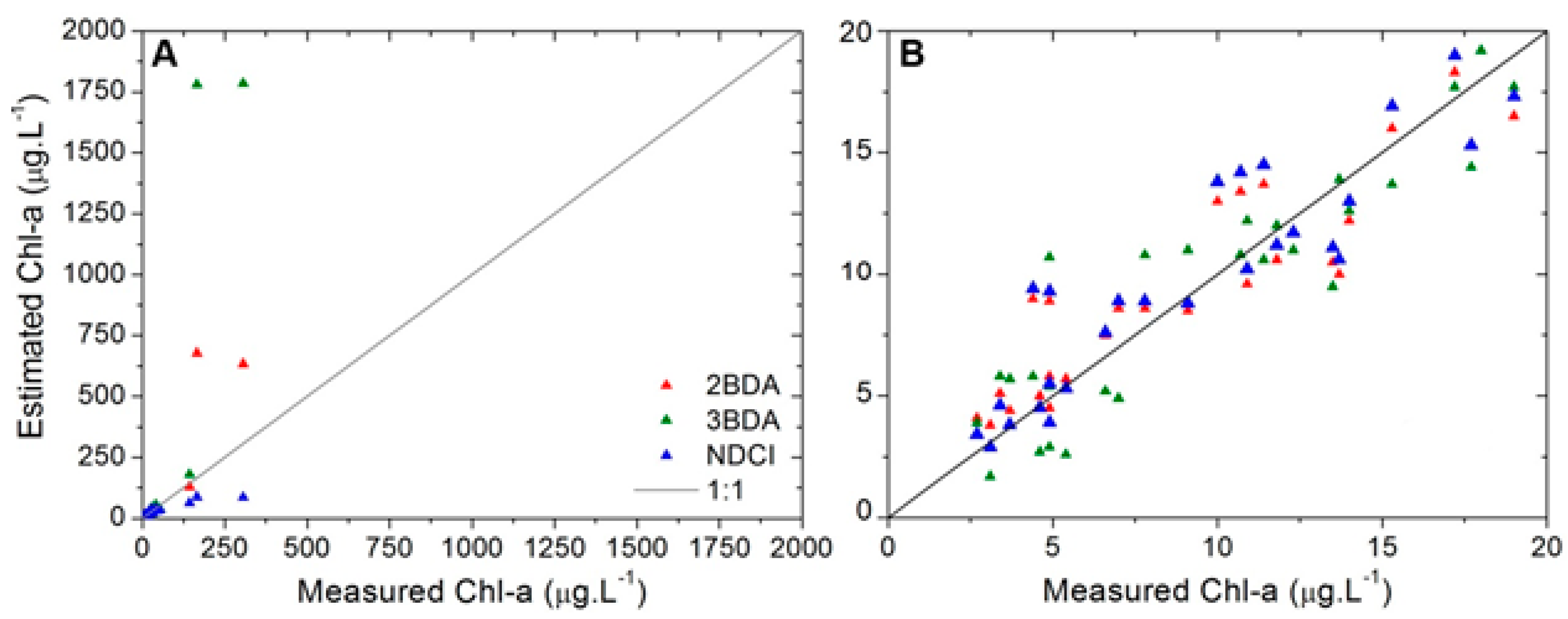
The scatterplot on Figure 9 shows that all algorithms diverge from 1:1 line and the error became greater as the chl-a concentration increases. This indicates that the parameterization found for these models using the whole range of chl-a concentrations can lead to inaccurate estimations of this parameter.

Figure 9. Scatterplots of the measured vs. estimated chl-a for each model using all in situ hyperspectral data. (A) All chl-a range; (B) Limiting the range to clarify the analysis.

Figure 9. Scatterplots of the measured vs. estimated chl-a for each model using all in situ hyperspectral data. (A) All chl-a range; (B) Limiting the range to clarify the analysis.

3.2.3. Calibration and Validation of OLCI Simulated Data

We simulated OLCI bands for the 28 samples with chl-a values under 20 µg∙L⁻¹. With these simulated bands, we repeated the calibration/validation process. Table 8 shows the calibration results for OLCI simulated bands. Analyzing the coefficients we notice the same pattern from hyperspectral calibration: the only model that had a negative intercept was 2BDA.

Table 8. Coefficients derived from model calibrations applied to OLCI simulated bands.

	Slope	Intercept	R²
2BDA	45.4	−16.3	0.90
3BDA	646.8	27.1	0.90
NDCI	57.7	25.7	0.90

Table 8. Coefficients derived from model calibrations applied to OLCI simulated bands.

	Slope	Intercept	R²
2BDA	45.4	−16.3	0.90
3BDA	646.8	27.1	0.90
NDCI	57.7	25.7	0.90

Figure 10 shows the histograms of the R² distribution obtained from Monte Carlo simulation. Again, the most frequent R² range was between 0.8 and 0.9. Among this range, we chose the best equation in validation.

Figure 10. Histograms of the R² distribution for: (A) May 2012; (B) September 2012; and (C) April 2013. OLCI simulated data with no chl-a below 20 µg∙L⁻¹.

Figure 10. Histograms of the R² distribution for: (A) May 2012; (B) September 2012; and (C) April 2013. OLCI simulated data with no chl-a below 20 µg∙L⁻¹.

The equations in Table 8 were validated and the results are in Table 9. NDCI had the best validation performance, with NRMSE% of 17.64%. This value is lower than what we found for NDCI using in situ hyperspectral data (17.85%, Table 5). This may be due to the band response as the positions of the chl-a features may shift and this may affect the in situ hyperspectral results. Based on the p value in Table 9 obtained by t test, no significant difference between the estimated and the measured chl-a concentration was found for all algorithms for a significance level of 5%.

Table 9. Summary results for validation process applied to OLCI simulated bands.

	Bias (µg∙L−1)	RMSE (µg∙L−1)	NRMSE%	p Value
2BDA	−0.02	2.88	18.07	0.982
3BDA	−0.03	3.23	20.27	0.978
NDCI	0.05	2.81	17.64	0.957

Table 9. Summary results for validation process applied to OLCI simulated bands.

	Bias (µg∙L−1)	RMSE (µg∙L−1)	NRMSE%	p Value
2BDA	−0.02	2.88	18.07	0.982
3BDA	−0.03	3.23	20.27	0.978
NDCI	0.05	2.81	17.64	0.957

The scatterplot showed in Figure 11 represents the measured chl-a concentrations versus the estimated ones. From it and the results in Table 9 it is evident that the best results were one more time obtained by NDCI and 2BDA models.

Figure 11. Scatterplots of the measured vs. estimated chl-a using OLCI simulated bands.

Figure 11. Scatterplots of the measured vs. estimated chl-a using OLCI simulated bands.

For 2BDA and 3BDA, the results shown in this paper contrast with the ones found for Gitelson et al. [8]. The authors observed that 2BDA is suitable for chl-a estimation in waters with chl-a values greater than 20 µg∙L⁻¹. In this paper, we observed that 2BDA is adequate for chl-a estimation in Funil reservoir with samples under 20 µg∙L⁻¹.

The reduced efficiency of 3BDA compared with 2BDA may be explained by its third band. This third band centered in 753 nm is minimally affected by chl-a, NAP and DOM absorption. Therefore, the total absorption at this wavelength is a measure of the absorption by water, i.e., the absorption at this wavelength is greater than the backscattering [8] which makes it responsible for minimizing the backscattering effect by NAP. The 2BDA model is a special case of 3BDA conceptual model when the absorption by chl-a is greater than the backscattering and also greater than the sum of NAP and DOM absorptions [8,19]. Matching these provisions, the explanation for 2BDA better performance may be that the inorganic suspended sediments (ISS) are negligible; and the organic suspended sediment (OSS) is correlated to chl-a.

Analyzing the SS field data, we observed that ISS are solely not negligible when we reach the river inlet, where we had a gradient of ISS in the inlet declining towards the dam. In addition, if we analyze the chl-a relationship with OSS excluding the sampling points located in the river inlet, which are mostly influenced by the river influx, we observed that they are correlated, with R² equals 0.86. These may be the reasons why the 2BDA performed better than the 3BDA for Funil reservoir.

Another explanation relies on the assumption of the spectral uniformity of backscattering coefficient over the wavelengths. Such assumption may not be true for inland turbid waters [39,40]. This would affect the accuracy of 3BDA at low chl-a concentrations as the third 3BDA band should remove the effects of particulate backscattering.

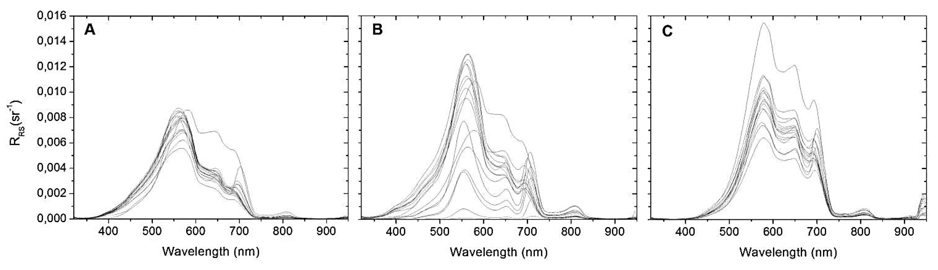
NDCI had the better performance probably due its structure: the difference between the chl-a absorption peak and chl-a reflectance peak, normalized by its sum. Based on the spectral architecture of this model, and the fact that its results are normalized, it is clear that it is sensitive to the difference between R_RS (709 nm) and R_RS (665 nm). As observed in Figure 2, these features are well marked in all data, which makes this model also suitable for Funil reservoir.

3.3. Comparison with Other Studies

Table 10 [8,9,12,41] shows different values of slope and intercept found on other studies. It is clear that the values diverge from each other with the change of study area. This was expected due to the empirical structure of the algorithms and the regional differences found among all study sites. The majority of studies available were performed in lakes and reservoirs located in temperate zones. Algorithms validation should be performed in other tropical inland waters to be able to compare the results found in this study. The spread of these studies will contribute to the ongoing development of algorithms adequate for tropical inland waters.

Table 10. Comparison of Slope and Intercept values from other studies.

Model	Reference	Location	Slope	Intercept
2BDA	This study	Funil reservoir	41.8	−15
	Mishra and Mishra [12]	Chesapeake Bay and Delaware Bay	20.96	−8.88
	Moses et al. [9]	Azov Sea	0.00002	0.61
	Gitelson et al. [8]	Nebraska and Iowa Reservoirs	0.95	4.55
	Gitelson et al. [8]	Nebraska Reservoirs	0.94	12.1
	Gitelson et al. [8]	Lake Minnetonka	0.94	6.82
	Gitelson et al. [8]	Choptank River	0.98	11.91
	Huang et al. [41]	5 Lakes in China	64.01	−46.19
3BDA	This study	Funil reservoir	581.1	25.5
	Mishra and Mishra [12]	Chesapeake Bay and Delaware Bay	136.13	11.52
	Gitelson et al. [8]	Nebraska and Iowa Reservoirs	0.89	2.84
	Gitelson et al. [8]	Nebraska Reservoirs	0.95	4.57
	Gitelson et al. [8]	Lake Minnetonka	1.07	-2.39
	Gitelson et al. [8]	Choptank River	0.96	3.33
	Huang et al. [41]	5 Lakes in China	90.05	19.63
NDCI	This study	Funil reservoir	54	23.8
	Mishra and Mishra [12]	Chesapeake Bay and Delaware Bay	87.99	13.55

Table 10. Comparison of Slope and Intercept values from other studies.

Model	Reference	Location	Slope	Intercept
2BDA	This study	Funil reservoir	41.8	−15
	Mishra and Mishra [12]	Chesapeake Bay and Delaware Bay	20.96	−8.88
	Moses et al. [9]	Azov Sea	0.00002	0.61
	Gitelson et al. [8]	Nebraska and Iowa Reservoirs	0.95	4.55
	Gitelson et al. [8]	Nebraska Reservoirs	0.94	12.1
	Gitelson et al. [8]	Lake Minnetonka	0.94	6.82
	Gitelson et al. [8]	Choptank River	0.98	11.91
	Huang et al. [41]	5 Lakes in China	64.01	−46.19
3BDA	This study	Funil reservoir	581.1	25.5
	Mishra and Mishra [12]	Chesapeake Bay and Delaware Bay	136.13	11.52
	Gitelson et al. [8]	Nebraska and Iowa Reservoirs	0.89	2.84
	Gitelson et al. [8]	Nebraska Reservoirs	0.95	4.57
	Gitelson et al. [8]	Lake Minnetonka	1.07	-2.39
	Gitelson et al. [8]	Choptank River	0.96	3.33
	Huang et al. [41]	5 Lakes in China	90.05	19.63
NDCI	This study	Funil reservoir	54	23.8
	Mishra and Mishra [12]	Chesapeake Bay and Delaware Bay	87.99	13.55

Table 11 [8,12,41,42,43] contains the comparison of the errors found in other studies. Analyzing the RMSE and the NRMSE we can see that the errors found in this study are coherent to other studies and in average lower than most of them. The NRMSE (or relative RMSE) is the most adequate error indicator to conduct a comparison, since it is normalized within the range of data from each study site. Nevertheless, it is not a very common error measure, which is why some studies lack this information.

Table 11. Comparison of error estimators values from other studies.

Model	Reference	Location	RMSE	NRMSE
2BDA	This study	Funil	2.92	18.32
	Mishra and Mishra [12]	Chesapeake Bay and Delaware Bay	2.82
	Moses et al. [42]	Azov Sea	6.04
	Gitelson et al. [8]	Nebraska and Iowa Reservoirs	10.2	36.2
	Gitelson et al. [8]	Nebraska Reservoirs	14.8	57.3
	Gitelson et al. [8]	Lake Minnetonka	6.15	25.3
	Gitelson et al. [8]	Choptank River	10.7	15.2
	Huang et al. [41]	5 Lakes in China	13.17	53.59
3BDA	This study	Funil	3.14	19.68
	Mishra and Mishra [12]	Chesapeake Bay and Delaware Bay	2.69
	Moses et al. [42]	Azov Sea	6.68
	Gitelson et al. [8]	Nebraska and Iowa Reservoirs	8.7	52.6
	Gitelson et al. [8]	Nebraska Reservoirs	11.2	46
	Gitelson et al. [8]	Lake Minnetonka	4.2	20.7
	Gitelson et al. [8]	Choptank River	6	47.9
	Huang et al. [41]	5 Lakes in China	12.58	51.19
NDCI	This study	Funil	2.84	17.85
	Mishra and Mishra [12]	Chesapeake Bay and Delaware Bay	1.43
	Zhang et al. [43]	Lake Taihu	6.48
	Zhang et al. [43]	Lake Taihu	22.53
	Zhang et al. [43]	Lake Taihu	5.73

Table 11. Comparison of error estimators values from other studies.

Model	Reference	Location	RMSE	NRMSE
2BDA	This study	Funil	2.92	18.32
	Mishra and Mishra [12]	Chesapeake Bay and Delaware Bay	2.82
	Moses et al. [42]	Azov Sea	6.04
	Gitelson et al. [8]	Nebraska and Iowa Reservoirs	10.2	36.2
	Gitelson et al. [8]	Nebraska Reservoirs	14.8	57.3
	Gitelson et al. [8]	Lake Minnetonka	6.15	25.3
	Gitelson et al. [8]	Choptank River	10.7	15.2
	Huang et al. [41]	5 Lakes in China	13.17	53.59
3BDA	This study	Funil	3.14	19.68
	Mishra and Mishra [12]	Chesapeake Bay and Delaware Bay	2.69
	Moses et al. [42]	Azov Sea	6.68
	Gitelson et al. [8]	Nebraska and Iowa Reservoirs	8.7	52.6
	Gitelson et al. [8]	Nebraska Reservoirs	11.2	46
	Gitelson et al. [8]	Lake Minnetonka	4.2	20.7
	Gitelson et al. [8]	Choptank River	6	47.9
	Huang et al. [41]	5 Lakes in China	12.58	51.19
NDCI	This study	Funil	2.84	17.85
	Mishra and Mishra [12]	Chesapeake Bay and Delaware Bay	1.43
	Zhang et al. [43]	Lake Taihu	6.48
	Zhang et al. [43]	Lake Taihu	22.53
	Zhang et al. [43]	Lake Taihu	5.73

3.4. MERIS Models Applied to OLCI Simulated Dataset

As a summary of the results, both 2BDA and NDCI showed adequate performance for chl-a concentration below 20µg∙L⁻¹: 2BDA had low NRMSE% (18.07%) and a negative intercept (−16.3); and NDCI had the lowest NRMSE% (17.64%). These results showed that OLCI will continue MERIS’ water quality monitoring legacy through previously published MERIS bio-optical models. This continuity is important for ongoing studies. The biggest problem of this sensor will be its spatial resolution, which will be the same as MERIS (300 m). This restricts the use of such data to water bodies with larger surface area. However, water quality monitoring by this sensor will be better because of the constellation structure of Sentinel 3 satellites which will improve the temporal resolution of their sensors and the extra bands which will provide improved models.

4. Conclusions

This study aimed to test the performance of the MEdium Resolution Imaging Spectrometer (MERIS) chlorophyll-a bio-optical models applied to in situ hyperspectral data and to the Ocean Land Color Instrument (OLCI) simulated data. We analyzed the performance of three published reflectance based algorithms to retrieve chlorophyll-a concentration already parameterized to fit MERIS bands. The models were evaluated for three conditions: i. hyperspectral data collected in situ with chlorophyll-a bellow 20 µg∙L⁻¹; ii. all hyperspectral data with no chlorophyll-a concentration limit; and iii. OLCI simulated data with chlorophyll -a bellow 20 µg∙L⁻¹.

Using chlorophyll-a concentration and hyperspectral data with concentration below 20 µg∙L⁻¹, the two band model (2BDA) proposed by Gitelson [19] had a low Normalized Root Mean Square Error in percentage (NRMSE% = 18.32%) and a negative intercept; and the Normalized Difference Chlorophyll Index (NDCI) proposed by Mishra and Mishra [12] had the lowest NRMSE% (17.85%).

Without restraining chl-a concentration, the Root Mean Square Error (RMSE) increased more than 300%, 1000% and 1500% for 2BDA, 3BDA (three band model proposed by Gitelson et al. [36]) and NDCI, respectively. This indicates that applying the same algorithm for a dataset with normal and bloom conditions can increase the errors of the chlorophyll-a estimation.

We also applied the hyperspectral data with concentration below 20 µg∙L⁻¹ to OLCI response function to test it using MERIS reflectance based bio-optical models. We found the same pattern showed for the hyperspectral data: 2BDA had a low NRMSE% (18.07%) and a negative intercept; and NDCI had the lowest NRMSE% among all (17.64%).

References

1. Tundisi, J.G.; Matsumura-Tundisi, T.; Tundisi, J.E.M. Reservoirs and human wellbeing: New challenges for evaluating impacts and benefits in the neotropics. Braz. J. Biol. 2008, 68, 1133–1135. [Google Scholar] [CrossRef] [PubMed]
2. Campbell, G.; Phinn, S.R.; Dekker, A.G.; Brando, V.E. Remote sensing of water quality in an Australian tropical freshwater impoundment using matrix inversion and MERIS images. Remote Sens. Environ. 2011, 115, 2402–2414. [Google Scholar] [CrossRef] [Green Version]
3. Gons, H.J.; Auer, M.T.; Effler, S.W. MERIS satellite chlorophyll mapping of oligotrophic and eutrophic waters in the Laurentian Great Lakes. Remote Sens. Environ. 2008, 112, 4098–4106. [Google Scholar] [CrossRef]
4. Kirk, J.T.O. Light and Photosynthesis in Aquatic Ecosystems; Cambridge University Press: Cambridge, UK, 1994. [Google Scholar]
5. Gitelson, A.A. The peak near 700 nm on radiance spectra of algae and water: Relationships of its magnitude and position with chlorophyll concentration. Int. J. Remote Sens. 1992, 13, 3367–3373. [Google Scholar] [CrossRef]
6. Richardson, L.L. Remote Sensing of algal bloom dynamics: New research fuses remote sensing of aquatic ecosystems with algal accessory pigment analysis. BioScience 1996, 46, 492–501. [Google Scholar] [CrossRef]
7. Mobley, C.D. Light and Water: Radiative Transfer in Natural Waters; Academic Press: San Diego, CA, USA, 1994. [Google Scholar]
8. Gitelson, A.A.; Dall’Olmo, G.; Moses, W.; Rundquist, D.C.; Barrow, T.; Fisher, T.R.; Gurlin, D.; Holz, J. A simple semi-analytical model for remote estimation of chlorophyll-a in turbid waters: Validation. Remote Sens. Environ. 2008, 112, 3582–3593. [Google Scholar] [CrossRef]
9. Moses, W.J.; Gitelson, A.A.; Berdnikov, S.; Povazhnyy, V. Estimation of chlorophyll-a concentration in case II waters using MODIS and MERIS data—Successes and challenges. Environ. Res. Lett. 2009, 4, 045005–045013. [Google Scholar] [CrossRef]
10. Le, C.; Li, Y.; Zha, Y.; Sun, D.; Huang, C.; Lu, H. A four-band semi-analytical model for estimating chlorophyll a in highly turbid lakes: The case of Taihu Lake, China. Remote Sens. Environ. 2009, 113, 1175–1182. [Google Scholar] [CrossRef]
11. Shen, F.; Zhou, Y.-X.; Li, D.-J.; Zhu, W.-J. Suhyb Salama, M. Medium resolution imaging spectrometer (MERIS) estimation of chlorophyll-a concentration in the turbid sediment-laden waters of the Changjiang (Yangtze) Estuary. Int. J. Remote Sens. 2010, 31, 4635–4650. [Google Scholar] [CrossRef]
12. Mishra, S.; Mishra, D.R. Normalized difference chlorophyll index: A novel model for remote estimation of chlorophyll-a concentration in turbid productive waters. Remote Sens. Environ. 2012, 117, 394–406. [Google Scholar] [CrossRef]
13. Matthews, M.W.; Bernard, S.; Robertson, L. An algorithm for detecting trophic status (chlorophyll-a), cyanobacterial dominance, surface scums and floating vegetation in inland and coastal waters. Remote Sens. Environ. 2012, 124, 637–652. [Google Scholar] [CrossRef]
14. Matthews, M.W. A current review of empirical procedures of remote sensing in inland and near-coastal transitional waters. Int. J. Remote Sens. 2011, 32, 6855–6899. [Google Scholar] [CrossRef]
15. Odermatt, D.; Gitelson, A.; Brando, V.E.; Schaepman, M. Review of constituent retrieval in optically deep and complex waters from satellite imagery. Remote Sens. Environ. 2012, 118, 116–126. [Google Scholar] [CrossRef] [Green Version]
16. Gordon, H.R.; Morel, A. Remote assessment of ocean color for interpretation of satellite visible imagery. In Lecture Notes on Coastal and Estuarine Studies; Barber, R.T., Mooers, C.N.K., Bowman, M.J., Zeitzschel, B., Eds.; Springer: New York, NY, USA, 1983; p. 114. [Google Scholar]
17. O’Reilly, J.E.; Maritorena, S.; Mitchell, B.G.; Siegel, D.A.; Carder, K.L.; Garver, S.A.; Kahru, M.; McClain, C. Ocean color chlorophyll algorithms for SeaWiFS. J. Geophys. Res. 1998, 103, 24937–24953. [Google Scholar] [CrossRef]
18. Campbell, J.; Antoine, D.; Armstrong, R.; Arrigo, K.; Balch, W.; Barber, R.; Behrenfeld, M.; Bidigare, R.; Bishop, J.; Carr, M.-E.; et al. Comparison of algorithms for estimating ocean primary production from surface chlorophyll, temperature, and irradiance. Global Biogeochem. Cycle. 2002. [Google Scholar] [CrossRef]
19. Dall’Olmo, G.; Gitelson, A.A. Effect of bio-optical parameter variability on the remote estimation of chlorophyll-a concentration in turbid productive waters: Experimental results. Appl. Opt. 2005, 44, 412–422. [Google Scholar] [PubMed]
20. MERIS. Product Handbook; European Space Agency (ESA): Paris, France, 2006. [Google Scholar]
21. Donlon, C.; Berruti, B.; Buongiorno, A.; Ferreira, M.-H.; Féménias, P.; Frerick, J.; Goryl, P.; Klein, U.; Laur, H.; Mavrocordatos, C.; et al. The global monitoring for environment and security (GMES) sentinel-3 mission. Remote Sens. Environ. 2012, 120, 37–57. [Google Scholar] [CrossRef]
22. Furnas. Sistema Furnas de Geração e Transmissão. Available online: http://www.furnas.com.br/hotsites/sistemafurnas/usina_hidr_funil.asp (accessed on 28 February 2013).
23. Primo, A.R.R. Avaliação da influência do reservatório de Funil na qualidade da água do rio Paraíba do Sul. Master’s Thesis, Universidade de São Paulo, Paulo, Brazil, 2006. [Google Scholar]
24. Instituto Estadual do Ambiente (INEA). Avaliação ambiental do Rio Paraíba do Sul; INEA: Rio de Janeiro, Brazil, 2010. [Google Scholar]
25. Bobeda, C. Isolamento, Purificação e Caracterização de Microcistinas (Hepta-Peptídeos Tóxicos) Encontrados em uma Floração de Cianobactérias Ocorrida no Reservatório do Funil. Master’s Thesis, Universidade Federal do Rio de Janeiro, Rio de Janeiro, Brazil, 1983. [Google Scholar]
26. Governo do Estado do Rio de Janeiro. Programa Estadual de Investimentos da Bacia do Rio Paraíba do Sul-RJ; Diagnóstico Ambiental; Fundação Superintendência Estadual de Rios e Lagoas (SERLA), Secretaria de Estado de Meio Ambiente: Rio de Janeiro, Brasil, 1997.
27. Rocha, M.I.A.; Branco, C.W.C.; Sampaio, G.F.; Gômara, G.A.; De Filippo, R. Spatial and temporal variation of limnological features, Microcystis aeruginosa and zooplankton in a eutrophic reservoir (Funil Reservoir, Rio de Janeiro). Acta Limnol. Brasil. 2002, 14, 73–76. [Google Scholar]
28. Novo, E.; Stech, J.; Alcântara, E.H.; Londe, L.; Assireu, A.; Barbosa, C. Integração de dados do Sistema de Monitoramento Automático de Variáveis Ambientais (SIMA) e de imagens orbitais na avaliação do estado trófico do reservatório da UHE funil. Geografia 2010, 35, 641–660. (in Portuguese). [Google Scholar]
29. TriOS. RAMSES Hyperspectral Radiometer Manual; TriOS Optical Sensor: Rastede, Germany, 2010. [Google Scholar]
30. Hooker, S.; Lazin, G.; Zibord, G.; McLean, S. An evaluation of above- and in-water methods for determining water-leaving radiances. J. Atmos. Ocean. Technol. 2002, 19, 486–515. [Google Scholar] [CrossRef]
31. Mobley, C.D. Estimation of the remote-sensing reflectance from above-surface measurements. Appl. Opt. 1999, 38, 7442–7455. [Google Scholar] [CrossRef]
32. Ohde, T.; Siegel, H. Derivation of immersion factors for the hyperspectral TriOS radiance sensor. J. Opt. A: Pure Appl. Opt. 2003, 5, L12–L14. [Google Scholar] [CrossRef]
33. Nush, E.A. Comparison of different methods for chlorophyll and phaeopigment determination. Arch. Hydrobiol. Beih. Ergebn. Limnol. 1980, 14, 14–36. [Google Scholar]
34. Lorenzen, C.J. Determination of chlorophyll and pheo-pigments: Spectrophotometric equations. Limnol. Oceanogr. 1967, 12, 343–346. [Google Scholar] [CrossRef]
35. Gons, H.J. Optical teledetection of chlorophyll a in turbid inland waters. Environ. Sci. Technol. 1999, 33, 1127–1132. [Google Scholar] [CrossRef]
36. Gitelson, A.A.; Gritz, U.; Merzlyak, M.N. Relationships between leaf chlorophyll content and spectral reflectance and algorithms for non-destructive chlorophyll assessment in higher plant leaves. J. Plant Physiol. 2003, 160, 271–282. [Google Scholar] [CrossRef] [PubMed]
37. Wynne, T.T.; Stumpf, R.P.; Tomlinson, M.C.; Warner, R.A.; Tester, P.A.; Dyble, J.; Fahnenstiel, G.L. Relating spectral shape to cyanobacterial blooms in the Laurentian Great Lakes. Int. J. Remote Sens. 2008, 29, 3665–3672. [Google Scholar] [CrossRef]
38. Schalles, J.F.; Yacobi, Y.Z. Remote detection and seasonal patterns of phycocyanin, carotenoid, and chlorophyll pigments in eutrophic waters. Arch. Hydrobiol. 2000, 55, 153–168. [Google Scholar]
39. Yacobi, Y.Z.; Moses, W.J.; Kaganovsky, S.; Sulimani, B.; Leavitt, B.C.; Gitelson, A.A. NIR-red reflectance-based algorithms for chlorophyll-a estimation in mesotrophic inland and coastal waters: Lake Kinneret case study. Water Res. 2011, 45, 2428–2436. [Google Scholar] [CrossRef] [PubMed]
40. Aas, E.; Høkedal, J.; Sørensen, K. Spectral backscattering coefficient in coastal waters. Int. J. Remote Sens. 2005, 26, 331–343. [Google Scholar] [CrossRef]
41. Huang, C.; Zou, J.; Li, Y.; Yang, H.; Shi, K.; Li, J.; Wang, Y.; Chena, X.; Zheng, F. Assessment of NIR-red algorithms for observation of chlorophyll-a in highly turbid inland waters in China. ISPRS J. Photogramm. Remote Sens. 2014, 93, 29–39. [Google Scholar] [CrossRef]
42. Moses, W.J.; Gitelson, A.A.; Berdnikov, S.; Saprygin, V.; Povazhnyi, V. Operational MERIS-based NIR-red algorithms for estimating chlorophyll-a concentrations in coastal waters—The Azov Sea case study. Remote Sens. Environ. 2012, 121, 118–124. [Google Scholar] [CrossRef]
43. Zhang, Y.; Ma, R.; Duan, H.; Loiselle, S.; Xu, J. A spectral decomposition algorithm for estimating chlorophyll-a concentrations in Lake Taihu, China. Remote Sens. 2014, 6, 5090–5106. [Google Scholar] [CrossRef]