From Remotely Sensed Vegetation Onset to Sowing Dates: Aggregating Pixel-Level Detections into Village-Level Sowing Probabilities

Abstract

Monitoring the start of the crop season in Sahel provides decision makers with valuable information for an early assessment of potential production and food security threats. Presently, the most common method for the estimation of sowing dates in West African countries consists of applying given thresholds on rainfall estimations. However, the coarse spatial resolution and the possible inaccuracy of these estimations are limiting factors. In this context, the remote sensing approach, which consists of deriving green-up onset dates from satellite remote sensing data, appears as an interesting alternative. It builds upon a novel statistic model that translates vegetation onset detections derived from MODIS time series into sowing probabilities at the village level. Results for Niger show that this approach outperforms the standard method adopted in the region based on rainfall thresholds.

1. Introduction

In Sahel, agricultural yields rely, among other factors, on the length of the crop season. Given millet photosensitivity and the limited variability of rainy season ending dates, late sowing is usually associated with shorter seasons [1] and consequently with lower crop yields [2,3,4]. Monitoring the start of the crop season provides decision makers with valuable information for an early assessment of potential production and food security threats. In such drought-prone regions, characterized by erratic early rainfalls, several systems to report or estimate crop progress stages (i.e., sowing dates) are operational, though often limited in their capacity to cover large areas with suitable precision and accuracy. Satellite imagery contributes to fill this gap since it potentially provides a periodical spatial overview of vegetation conditions and offers means for the estimation of phenological stages (see [5] for a review of the methods).

Presently, the most common method for the estimation of sowing dates in West African countries consists in applying given thresholds on rainfall quantity which is the main, even the only climatic factor affecting vegetation growth in Sahel. Following this agrometeorological approach, the assumption is that successful sowing occurs when rainfall exceeds 20 mm in a dekad (10-day period) and adds up to at least 20 mm in the following two dekads [2,6]. The rationale of this rule is that it fairly corresponds to the behavior of farmers who usually sow after the first important rainfall event, but have to sow again if a dry spell jeopardizes crops at their early stages. However, two important drawbacks should be stressed: (i) the discrepancy between the spatial resolution of rainfall data (8 km) and the spatial micro-variability that characterizes rainfall in Sahel [7], and (ii) the possible inaccuracy of rainfall estimations [8,9,10]. The limited reliability of this method is evidenced by the substantial effort the government still puts into in loco assessments of sowing dates in 10,557 villages (out of 27,897 villages censed in the country).

In this context, the remote sensing approach that consists in deriving green-up onset dates from vegetation indices, e.g., the Normalized Difference Vegetation Index (NDVI) and the enhanced vegetation index (EVI), appears as an interesting alternative. Two advantages can be put forward: (i) a higher spatial resolution and (ii) the fact it integrates vegetation responses to various factors, including farmers decisions, and not only rainfall.

However, the use of vegetation indices also has its shortcomings [5,11,12,13,14]. Their sensitivity to soil background is a major concern [13] in arid and semi-arid regions with low sowing densities. Indeed, bare soils often have spectral characteristics that induce NDVI values similar to sparse vegetation ones [15,16]. Moreover, NDVI suffers from noise induced by atmospheric conditions [17,18,19] and from uncorrected directional viewing effects. The use of the middle-infrared (MIR) wavelength as a complement to the red and NIR can guarantee a more robust and reliable image-independent discrimination between vegetation and non-vegetation surface types [16]. Indeed, the MIR spectral band is sensitive to water content in the soil and vegetation [20] and therefore improves the discrimination between vegetation and surrounding bare soils that are usually drier. To deal with this, Pekel, et al. [21] propose an innovative multi-temporal and multi-spectral image analysis method based on the red, NIR and MIR channels, that guarantees a more robust and reliable discrimination between vegetated and non-vegetated surfaces. The approach offers a good basis to identify the transition from bare soils to vegetation covers at an early stage.

A plethora of methods have been proposed in the literature for the estimation of the start of the season (SOS) from satellite based phenology [22,23,24,25,26,27,28]. Heuristics for the detection of SOS include the use of thresholds on remote sensing derived rainfall [24], on the ratio between NDVI increase and NDVI maximum on smoothed seasonal observations [25] and on fitted functional forms [26]. Curve fitting approaches also use the minimal point [27] or curvature-change [23,28] as a proxy for the SOS. However, few studies tried to explicitly tie phenological information from remotely sensed time series to actual sowing dates. Brown and de Beurs [22] propose a phenological model tuned specifically to the semi-arid, monsoonal ecosystem of West African Sahel to identify the start of the season and validate the results with sowing dates from field observations. The highest correlation (R² > 0.8) between the derived SOS dates and the field observations were obtained with NDVI data aggregated at a spatial resolution of 8 km/pixel. The approach was however less efficient at a higher spatial resolution necessary for an assessment at the village level. Moreover, no model has been proposed to explicitly link satellite based phenology to ground data at the early stage of the season. Indeed, in the existing literature, the start of the season can only be determined when the season is completed, because fitting quadratic models (or other functional forms) requires observations in the growing phase as well as in the senescent phase, which is a major drawback for early warning assessments.

This study proposes an innovative statistical model that attributes sowing probabilities to villages based on surrounding green-ups as soon as they are detected. The sowing probabilities at a given date inform on the effective start of the crop-growing season and are updated throughout the season. The model maximizes the likelihood of observing the number of villages having sown per dekad at the department level, as officially reported by the Ministry of Agricultural Development of Niger (see next section). The originality of the approach consists in linking pixel level information with ground data aggregated at the department level in a sound theoretical framework. The identification of vegetation onsets follows the methodology described in [21] applied to the Moderate Resolution Imaging Spectroradiometer (MODIS) time series at 250 m. Years 2008 and 2009 are used for estimation and cross validation purposes. Results are compared to sowing dates obtained by applying the agrometeorological approach proposed by Sivakumar [1] to the rainfall estimates (RFE2) of the Climate Prediction Center/Famine Early Warning System (FEWS NET) [29].

2. Material and Methods

2.1. Data

In an effort towards a comprehensive assessment of the agricultural season, the Ministry of Agricultural Development (Ministère du Développement Agricole) of Niger periodically performs, all over the country, field visits for crop development monitoring. Information on rainfall, sowing dates, phenological development, planted and harvested areas as well as on yields is thus collected by agricultural extension officers and reported during the agricultural season. The collection of dekadal information on the number of villages having sown in each of the departments of the country (there are 36 departments in Niger with a median size of 7987 km²) takes place every year from April to July. The data is corrected for missed sowings due to consecutive dry-spells during subsequent field visits. Table 1 gives an overview of this data for the 2008 crop season, aggregated into seven regions for the sake of simplicity. Please notice the distinction between regions, the aggregation unit on Table 1, and departments, the aggregation unit at which data is available and is the basis for the analysis. We take it as ground truth and use the information at the department level for both the calibration of the statistical model and the cross validation procedure. Although recognizing the limitations of this dataset for validation purposes, we believe that one of the main contributions of this work is to propose an innovative statistical framework (see Subsection 2.4) that ties information at different scales −250 m pixels, 5 km buffer around villages and department—in a sound theoretical framework.

Table 1 shows the high heterogeneity in planting dates within regions, regardless of their size. Heterogeneity of similar amplitude is observed at our level of analysis (departments): in 2008, in Matameye (the smallest department in the country with less than 2500 km²) 23% of the villages had sown at the beginning of May while the last 20% of the villages had to wait until the first dekad of July in order to have a successful planting.

Table 1. Cumulated number of villages having sown per dekad and per region in 2008. The data is from [30].

Region	Total	April			May			June			July
		Dek1	Dek2	Dek3	Dek1	Dek2	Dek3	Dek1	Dek2	Dek3	Dek1	Dek2	Dek3
Diffa	600	0	0	0	0	0	0	0	0	170	450	600	600
Dosso	1448	0	0	6	60	337	744	798	1073	1442	1448	1448	1448
Maradi	2181	7	7	7	7	229	563	966	1391	1766	2091	2181	2181
Niamey	34	0	0	0	0	0	17	17	30	34	34	34	34
Tahoua	1495	0	0	0	1	42	224	387	673	1078	1380	1493	1495
Tillabery	1849	0	0	0	3	73	279	710	1184	1783	1830	1849	1849
Zinder	2950	0	0	22	35	87	187	406	585	2077	2847	2932	2950
Niger a	10557	7	7	35	106	768	2014	3284	4936	8350	10080	10537	10557

^a except Agadez.

Table 1. Cumulated number of villages having sown per dekad and per region in 2008. The data is from [30].

Region	Total	April			May			June			July
		Dek1	Dek2	Dek3	Dek1	Dek2	Dek3	Dek1	Dek2	Dek3	Dek1	Dek2	Dek3
Diffa	600	0	0	0	0	0	0	0	0	170	450	600	600
Dosso	1448	0	0	6	60	337	744	798	1073	1442	1448	1448	1448
Maradi	2181	7	7	7	7	229	563	966	1391	1766	2091	2181	2181
Niamey	34	0	0	0	0	0	17	17	30	34	34	34	34
Tahoua	1495	0	0	0	1	42	224	387	673	1078	1380	1493	1495
Tillabery	1849	0	0	0	3	73	279	710	1184	1783	1830	1849	1849
Zinder	2950	0	0	22	35	87	187	406	585	2077	2847	2932	2950
Niger a	10557	7	7	35	106	768	2014	3284	4936	8350	10080	10537	10557

^a except Agadez.

From the remote sensing side, two datasets have been used: RFE 2.0 and four MODIS daily products from Aqua and Terra sensors. The first is a dekadal rainfall estimate at 8 km resolution available at the Climate Prediction Center/Famine Early Warning System. The second are the daily MODIS products (version 5, L2G), processed in order to maximize the number of cloud-free observations: the 250 m products (MYD09GQ and MOD09GQ) for the Red and the NIR bands, and the 500 m products (MYD09GA and MOD09GA) for the middle infrared (MIR) which is then resampled to 250 m.

In addition, the location of the Nigerien villages comes from the 2001 national census (Troisième Recensement Général de la Population et de l’Habitat, INS, Niger) during which most villages of the country have been georeferenced. The data provided by the National Institute of the Statistics (INS) of Niger was collected between the 20th May 2001 and the 10th June 2001 and covers the whole territory. The census lists up to 27,897 villages of which 83% are georeferenced. The georeferenced villages cover 94% of the total censed population of 11,060,291 inhabitants.

Finally, while sowing dates derived from rainfall estimates are directly attributed to the villages inside each 8 km pixel, vegetation onset detections are considered in buffers surrounding each village. In order to avoid the over-parameterization of the model, the optimal buffer has been defined a priori as the one that maximizes the agreement between the resulting village buffer mask (VBM; see Subsection 2.2 for details) and a reference crop mask (CM) [31]. The CM spatially combines the cropland classes with more than 30% of crops from the Cropland Use Intensity dataset (USGS, 1988) and the irrigated agriculture and plantation classes from the Land Use-Land Cover dataset (LULC, 2000), both resampled at 250 m.

2.2. Village Buffer Mask

As previously discussed, given the spatial variability of the sowing dates in Niger, the 250 m resolution of vegetation onsets derived from MODIS imagery (see next section) appears as an alternative to the coarse resolution of RFE 2.0 rainfall data. However, the plots of the same village are generally covered by several MODIS pixels so that a single MODIS pixel cannot encompass the dynamics of sowing in the village. The question is then how large is the area around each village where detected vegetation onsets carry information on the agricultural activities of the villagers. Instead of selecting the buffer size such as to maximize the performance of the statistical model or selecting a buffer size based on a subjective belief (e.g., “the plots are situated at a walking distance of maximum 1 h”), we have decided to rationalize the choice of the buffer by maximizing its agreement with a reference crop mask. This choice has the advantage of being objective while minimizing the risk of over-parameterization of the model, given the only two years of data available on sowing dates. The identification of the optimal buffer size has four steps:

• Exclusion of the villages outside the agricultural and agro-pastoral zones as defined by FEWS NET’s Niger Livelihood Profiles since sowing is not expected to happen in those;
• Generation of buffers of radius r in {1, 2, 3, …, 8} km around the villages located in the agricultural and agro-pastoral zones;
• Individual village buffers are merged in order to create eight so called village buffer masks (VBM), each one corresponding to a different buffer size;
• Computing the area covered by the crop mask, by each of the VBMs and the intersections between the crop mask and the VBMs.

We define agreement as the difference between (i) the percentage of the crop mask covered by the VBM and (ii) the percentage of the VBM not covered by the crop mask (i.e., the commission errors). The first component expresses the capacity of the VBM to cover agricultural areas and should be maximized. The second component, which should be as low as possible, measures the occurrence of non-agricultural areas among pixels later included in the analysis. Both components have, by definition, a positive, but not strictly positive, derivative with respect to the buffer size. Moreover, since agriculture has a higher likelihood to develop in the surroundings of the villages, for small/large buffers the percentage of the crop mask covered by them is expected to increase faster/slower with the buffer size than percentage of the VBM not covered by the crop mask. In other words, the difference between the two curves, or agreement, is a concave function that reaches its maximum at the optimal buffer size. The stylized Figure 1 summarizes this idea. This approach is based on an elegant formulation and has the advantage of providing a rational and objective criterion for the definition of an optimal buffer. Furthermore, this is a general approach and could also be used in other contexts and applications.

Figure 1. Stylized representation of the expected relationship between the buffer size around villages and (i) the surface of the crop mask covered by the resulting village buffer mask (green line) and (ii) the surface of the VBM not covered by the crop mask (orange line). The optimal buffer size maximizes the difference between the two curves and is represented by the point B^*.

Figure 1. Stylized representation of the expected relationship between the buffer size around villages and (i) the surface of the crop mask covered by the resulting village buffer mask (green line) and (ii) the surface of the VBM not covered by the crop mask (orange line). The optimal buffer size maximizes the difference between the two curves and is represented by the point B^*.

2.3. Onset Detections Derived from MODIS

Here we define the green-up onset stage as the transition from a bare surface to a vegetation surface. The main challenge for the identification of this transition is the automatic discrimination between non-vegetated and vegetated surfaces at an early stage of development (i.e., very low vegetation density). The possible confusion between bare soils and vegetation in arid and semi-arid areas, gives rise to the need for a qualitative index based on MIR, NIR, and red spectral bands. Moreover, the index should ideally identify green vegetation consistently and independently from observation conditions (atmosphere and acquisition geometry), and of its intrinsic variations (the phenological stage). Pekel, et al. [21] proposes such an index by using a colorimetric approach of the signal. This index, called hereafter Hue index, represents the Hue component after a color transformation of the RGB space (with the MIR wavelength in the R channel, the NIR in the G channel, and the Red in the B channel) into the Hue-Saturation-Value (HSV) system. The onset vegetation detection is based on the combination of this new index and the NDVI. In this two-dimensional space, the empirical discriminant lines have been identified based on a set of thresholds derived from a large sampling of pixels spread both in time and space in vegetated and non-vegetated areas (respectively 1,910,597 and 21,413,604 pixels). The approach presents four advantages that justifies its use for the dekadal detection of vegetation in our methodology: (i) it exploits the multi-spectral information and consequently avoids usual confusions between bare soils and vegetation, (ii) it synthetizes the multi-spectral information in one value, and (iii) it reduces the noise due to the observation conditions and (iv) it allows the identification of the transition from bare soils to vegetation covers at an early stage.

The processing chain applied on the daily MODIS images includes 5 steps. (i) For each sensor (i.e., Aqua and Terra), the compositing of daily images on a 10-day basis using the mean compositing strategy [32]. (ii) The resampling to 250 m of the MIR channel (nearest-neighbor resampling). (iii) The computation of two vegetation indices: the NDVI and the Hue index, using three reflectance bands, i.e., MIR, NIR, and red [21]. (iv) The detection of vegetation based on a set of thresholds using jointly the Hue and the NDVI indices [21]. (v) The identification of the green-up onset dates based on the vegetation detections. As several vegetation onsets may be detected for the same pixel during a single crop season, only the last detection, interpreted as the successful planting, is used in the analysis, while previous detections are considered as failed plantings (e.g., due to a dry spell at an early stages of crop development). The analysis covers the period between 1 April and 20 August and later detections are neglected.

As a concluding remark, it is worth motivating the processing of daily images (the first step of the processing chain). First, it allows for the adaptation of the length of the compositing period to the user needs and location in order to optimize the number of cloud-free observations. In our study, the preparation of the 10-day composites was necessary because field data was also collected at a 10-day frequency. Second, we demonstrate the possibility to start from the daily data instead of the already packaged composites, a useful approach in the period of increased computing capacity, including online processing solutions like the one offered by Google Earth Engine. Finally, the MC presents some advantages compared to algorithms used in the standard products [32] such as the Nadir BRDF-Adjusted Reflectance (NBAR) MODIS products: (i) the mean reduces the BRDF effects and also the possible perturbations remaining after atmospheric correction and cloud removal, (ii) less cloud-free observations are needed, a significant advantage as the vegetation starts at the cloudiest season, and (iii) the higher spatial resolution (250 m instead of 500 m).

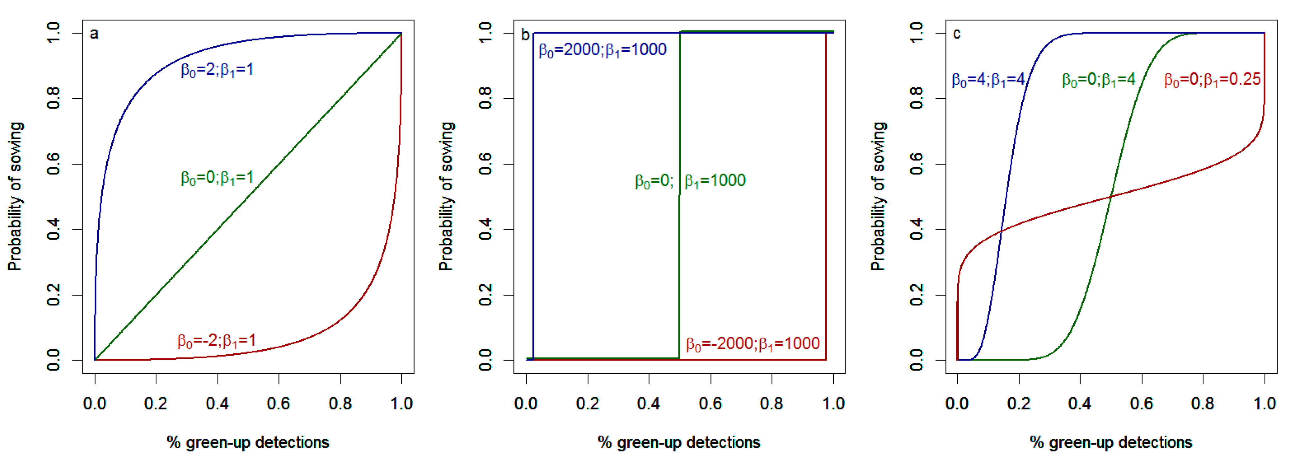
2.4. Statistical Framework

Once detected at the pixel level, vegetation onsets are to be translated into sowing dates. The task presents two major challenges: (i) how to efficiently aggregate the information at 250 m resolution into the predefined village buffers and (ii) how vegetation onset detections relate in time with sowing dates. The statistical framework hereafter described has been specifically designed to address these problems under the constraint of the validation data which informs about the number of villages having sown by dekad in each of the 36 departments. First, sowing is assessed as a probability (Equation (1)) that is proportional to the percentage of detected pixels around villages (Equations (2) and (3)). The function that links the percentage of detected pixels to a probability of sowing is general enough to accommodate a plethora of functional forms with the estimation of only two parameters (Figure 2). Finally, we define the resulting distribution of the number of villages having sown in a department as a function of the probabilities of sowing in the villages within it (Equation (5)) and we derive the corresponding log-likelihood function to be maximized (Equation (9)). This flexible but parsimonious specification guarantees that detections are efficiently translated into a probability of sowing over dekads.

Let us assume that the binary sowing variable s_i,k,t follows a Bernoulli process that equals 1 if the village i in department k has sown at or before time t; and 0 otherwise:

$$S_{i,k,t}~Be(P_{i,k,t})$$

(1)

where the parameter p_i,k,t, the probability of a sowing having taken place, is a function of V_i,k,t, the percentage of pixels where a vegetation onset has been detected at or before time t in the buffer surrounding the village i from department k:

$$p_{i,k,t}=Ф({\beta }_0+{\beta }_1{V^{\prime }}_{i,k,t})$$

(2)

with

$${V^{\prime }}_{i,k,t}={\varphi }^{-1}(V_{i,k,t})$$

(3)

where Ф and Ф⁻¹ have been respectively defined as the cumulative density function of a normal distribution and its inverse. Note that Equation 3 translates the percentage V_i,k,t from the interval [0,1] to the interval [−∞,∞], before being introduced in Equation (2). Conversely, Equation (2) translates V’_i,k,t back into a probability interval [0,1] after the coefficients to be estimated β₀ and β₁ come into play. This specification accommodates a vast diversity of relationships between the percentage of detected pixels and the probability of sowing (Figure 2).

Then, under independence of sowing assessments between villages:

$$S_{i,k,t}\perp S_{j,k,t}$$

(4)

Let us now define Y_k,t the total number of villages in the department k having sown at or before time t, following a Poison-Binomial distribution [33] with probabilities coming from Equation 2:

$$Y_{k,t}~PoBi(P_{i,k,t})$$

(5)

It follows that:

$${\mu }_{k,t}=\text{E}\left(Y_{k,t}\right)={\displaystyle \sum _{i=1}^{n^k}{p}_{i,k,t}}$$

(6)

is the expected value of Y_k,t and its variance is given by:

$${\sigma }_{k,t}^2={\displaystyle \sum _{i=1}^{n^k}{p}_{i,k,t}(1-p_{i,k,t})}$$

(7)

with n^k being the total number of villages in the department k. Since the condition of Lyapunov is fulfilled for a sum of independent Bernoulli trials, the central limit theorem can be generalized to the case of not identically distributed variables and Y_k,t converges in distribution to a normal distribution when n^k goes to infinity:

$$Y_{k,t}\stackrel{d}{\to }N({\mu }_{k,t},{\sigma }_{k,t}^2)$$

(8)

In our case, n ranging from 38 (Abalak) to 1850 (Miria), the Normal distribution has been used as a proxy for the Poisson-Binomial distribution (due to computational limitations) and parameters β₀ and β₁ can be found by maximizing the following log-likelihood function:

$$\underset{{\beta }_0,{\beta }_1}{\max }{\displaystyle \sum _{k=1}^d{\displaystyle \sum _{t=1}^T(-\frac{1}{2}\ln ({\sigma }_{k,t}^2)-\frac{{(Y_{k,t}-{\mu }_{k,t})}^2}{2{\sigma }_{k,t}^2})}}$$

(9)

As final remarks, the motivation for the statistical framework is twofold. First, it is a formal representation of the random process generating the available data on sowing dates: extension officers assess if “the village” has sown with a probability of yes that is proportional to the share of fields in the surroundings where a successful sowing took place (Equation (1)); this information is then aggregated and reported at the department level (Equations (5) and (6)).

Figure 2. Potential functional forms between the percentage of pixels for which a vegetation onset has been detected and the probability of a successful sowing. A high diversity of functional forms can be obtained with only two parameters. i.e., β₀ and β₁ in Equation (2). Linear, strictly positive and strictly negatives second derivatives with β₁ = 1 (a); threshold with β₁→∞ (b); and change in concavity with β₁ ≠ 1 (c). Only positive values of β₁ are considered.

Figure 2. Potential functional forms between the percentage of pixels for which a vegetation onset has been detected and the probability of a successful sowing. A high diversity of functional forms can be obtained with only two parameters. i.e., β₀ and β₁ in Equation (2). Linear, strictly positive and strictly negatives second derivatives with β₁ = 1 (a); threshold with β₁→∞ (b); and change in concavity with β₁ ≠ 1 (c). Only positive values of β₁ are considered.

Second, as the functional form that ties a percentage of fields with a probability of declaring the sowing is unknown, we proposed a generic framework where a plethora of relationships between the two variables can potentially be accommodated with the estimation of only two parameters. Figure 2 illustrates some of the cases. The first box (a) shows that, holding β₁ = 1, the concavity of the relationship varies with the sign and the magnitude of β₀. Then, in the second box (b) we see that high values of β₁ generate a threshold approach, where sowing is declared with 100% chance when the percentage of fields having sown exceed a given level. Note that it can be demonstrated analytically that the threshold equals Ф (β₀/β₁). Finally, the specification is flexible enough to model relationships with a change in concavity, both from positive to negative second derivatives (β₁ > 1) and from negative to positive second derivatives (β₁ < 1) as illustrated in the third box (c).

2.5. Rainfall Estimate for Sowing Dates

The most common method for estimating sowing dates in Sahel is the one proposed by [1]. The rationale of the method is that it fairly corresponds to the behavior of farmers who usually sow after the first important rainfall event occurring from May onwards. On a per pixel basis (8 km), a rainfall threshold criterion is applied to dekadal rainfall estimates (RFE 2.0) values. The assumption is that sowing happens in the first dekad (from May onwards) with at least 20 mm of rainfall. Moreover, a sowing is successful if and only if the aggregated rainfall during the next two dekads equals or exceeds 20 mm; otherwise, it is considered as a failure and the method searches for a new sowing. The last point implies that a sowing that takes place in dekad t is reported as successful two dekads later.

3. Results

3.1. Village Buffer Mask

Table 2 summarizes the results of the analysis detailed in Subsection 2.2. It shows for a series of buffer radius around villages (i) the percentage of the crop mask (CM) covered by village buffer mask (VBM), (ii) the percentage of VBM not covered by CM and (iii) the difference between both. The buffer that maximizes the last indicator is retained in the next steps of the analysis. As expected, for small buffers the percentage of CM covered by VBM increases faster than the percentage of VBM not covered by CM, and the opposite holds for large ones. The percentage of CM covered by VBM reaches values higher than 90% and for buffers superior to 5 km, a plateau zone appears, with increases inferior to 1%. In contrast, the increase of the percentage of VBM not covered by the CM is rather steady and never superior to 5%. As a result, the difference between both curves is a concave function and it reaches its maximum for buffers of around 5 km.

Indeed, in Niger, the vast majority of the plots are within a radius of four to five kilometers from the village. In addition, a buffer of 5 km corresponds to a 1-hour walking distance, which seems to be a relevant choice. Farther fields are usually not cultivated. We consequently adopt the 5 km buffers as a benchmark for the vegetation onset detection around villages. The resulting VBM covers 97.6% of the CM while 59.6% of it is not covered by the CM. This apparently large commission error can be the due to large agricultural areas that were not included in the CM either (i) because of the difficulty of visual interpretation when applied to arid and semi-arid areas where natural vegetation and/or fallow fields are usually highly mixed with and within crop fields or (ii) because the CM was created using outdated Landsat images (1988). It is worth noting that natural vegetation associated with crops can improve the scope of the use of green-up onset detections for the estimation of sowing dates in Sahel given the steeper reaction to moisture of the former and the low planting densities of the later. Early detections are then more likely to be successful.

Table 2. Overlaps and no-overlaps between the crop mask and village buffers mask for buffer sizes between 1 km and 8 km.

Variable		Buffer Size around Villages
		1 km	2 km	3 km	4 km	5 km	6 km	7 km	8 km
%CM Covered by the VBM	29.3		68.6	87.5	94.8	97.6	98.8	99.4	99.6
%VBM not Covered by the CM	42.8		47.7	53.1	57.0	59.6	61.2	62.4	63.3
Difference	−13.5		20.8	34.5	37.9	38.0	37.6	37.0	36.3

Table 2. Overlaps and no-overlaps between the crop mask and village buffers mask for buffer sizes between 1 km and 8 km.

Variable		Buffer Size around Villages
		1 km	2 km	3 km	4 km	5 km	6 km	7 km	8 km
%CM Covered by the VBM	29.3		68.6	87.5	94.8	97.6	98.8	99.4	99.6
%VBM not Covered by the CM	42.8		47.7	53.1	57.0	59.6	61.2	62.4	63.3
Difference	−13.5		20.8	34.5	37.9	38.0	37.6	37.0	36.3

3.2. Vegetation Onset Detections and Rainfall Thresholds

Figure 3 shows the results of the green-up onset dates derived from MODIS using the hue index and the estimated sowing dates derived from RFE for the two years, i.e., 2008 and 2009 respectively on the left and right hand side. As expected, the main differences between the two products are: (i) a delay between the RFE based sowing dates and the timing of vegetation onset detections, since the latter is the response of the vegetation to the first rains; (ii) the spatial resolution of the products, i.e., 8 km for RFE as opposed to 250 m for MODIS.

Figure 3. The dekad of the last green-up detection derived from MODIS for the whole country (a1) for 2008 and (a2) for 2009, and a zoom over Maradi region (see location box in a1) (a1’) for 2008 and (a2’) for 2009. The estimated sowing dekad derived from RFE for the whole country (b1) for 2008 and (b2) for 2009, and a zoom over Maradi region (b1’) for 2008 and (b2’) for 2009. The color white represents the areas where crops never started before 20 August. The black dots represent the villages.

Figure 3. The dekad of the last green-up detection derived from MODIS for the whole country (a1) for 2008 and (a2) for 2009, and a zoom over Maradi region (see location box in a1) (a1’) for 2008 and (a2’) for 2009. The estimated sowing dekad derived from RFE for the whole country (b1) for 2008 and (b2) for 2009, and a zoom over Maradi region (b1’) for 2008 and (b2’) for 2009. The color white represents the areas where crops never started before 20 August. The black dots represent the villages.

More importantly, images at the national scale (Figure 3a1,a2,b1,b2) show that the differences are not limited to a systematic delay of the vegetation onset detections, but that the spatial dynamics of the methods are also different. In some areas (south-west) vegetation green-up detections happened before the rainfall conditions have triggered. Interesting enough, it may happen both in the drier regions of the north and in the relatively more humid areas of the south (see the Western Dakoro in 2009 and Southern Gaya 2008). Clearly enough, the two methods do not provide the same information and that regardless the systematic delay and the spatial scale. Conclusions drawn from the first may substantially differ from the one coming from the second. Consequently, it is crucial to assess their respective performances.

Figure 3 zooms in Maradi (a1’, a2’, b1’, b2’), one of the most important regions for cereal production in the country. With the additional display of the village layer (black dots) in these images, the spatial discrepancy of the information on sowing dates at the village level that each product brings becomes evident. For instance, in the Aguié department, the RFE product almost entirely misses in both years the spatial variations of sowing dates captured by the vegetation onset product based on MODIS imagery. At this stage, it is impossible to determine if the problem is on the coarseness and inaccuracy of RFE data or if the spatial heterogeneity of MODIS-based green-up detections is simply an artifact that does not relate to the sowing practices on the ground. The next section aims at shading light on this question by using the number of villages that have sown at the department level for the calibration of the model. The MODIS-based green-up detections are then translated into actual (expected) sowing dates to be compared with the sowing dates derived from the 20 mm-rule.

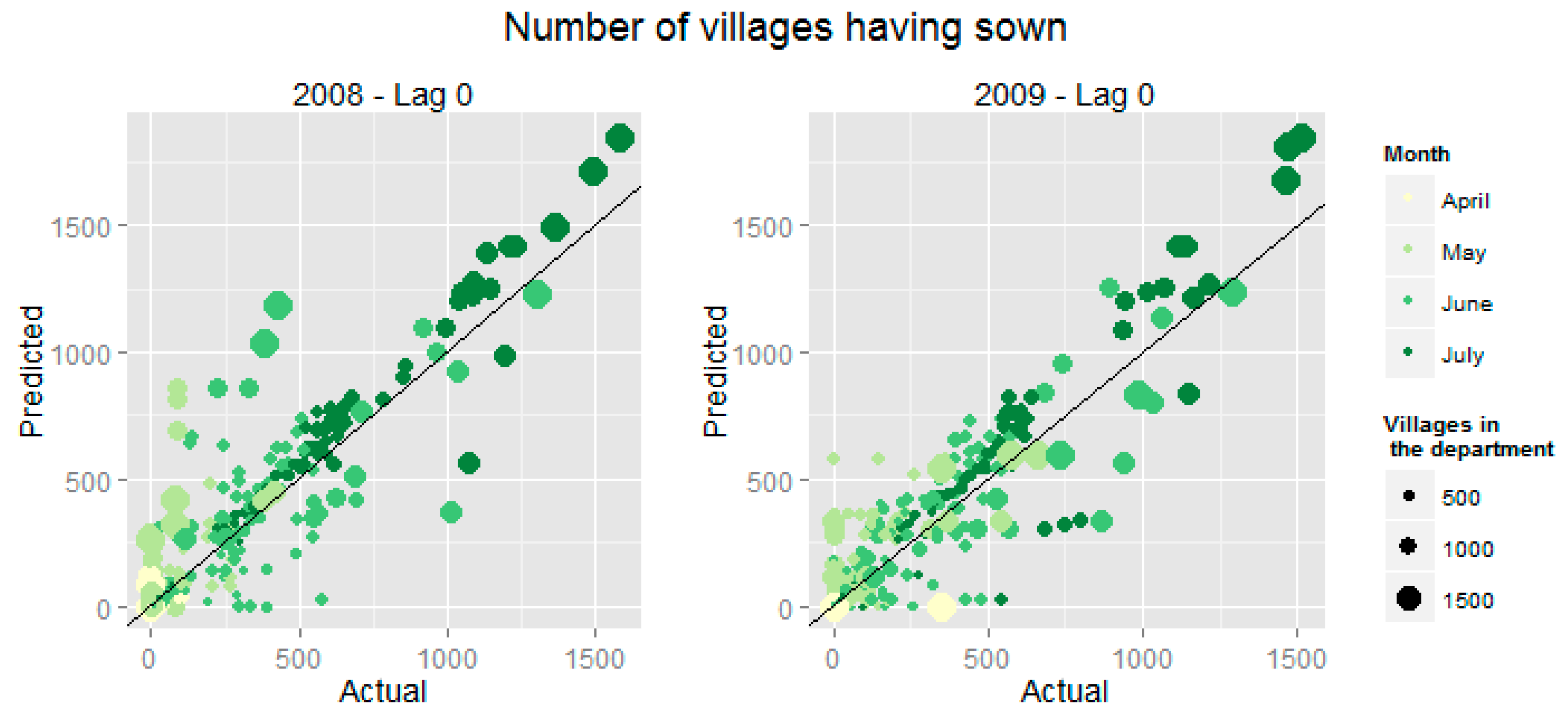
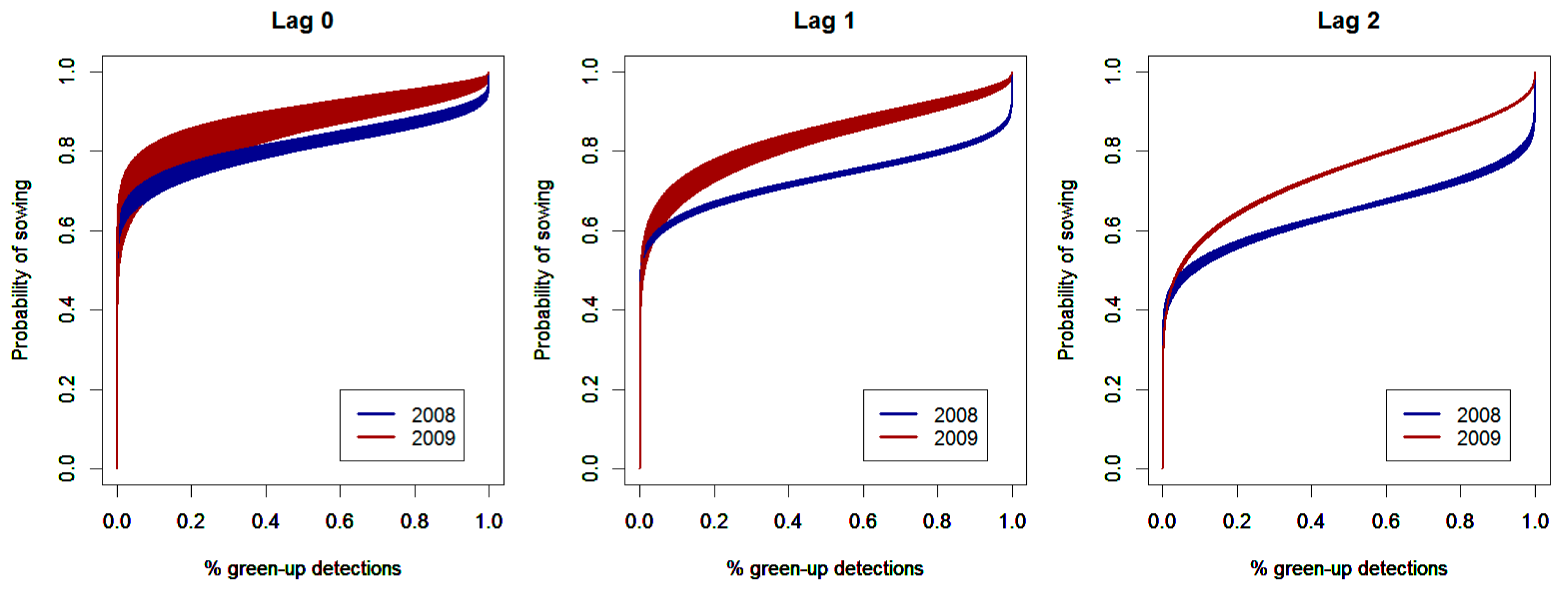
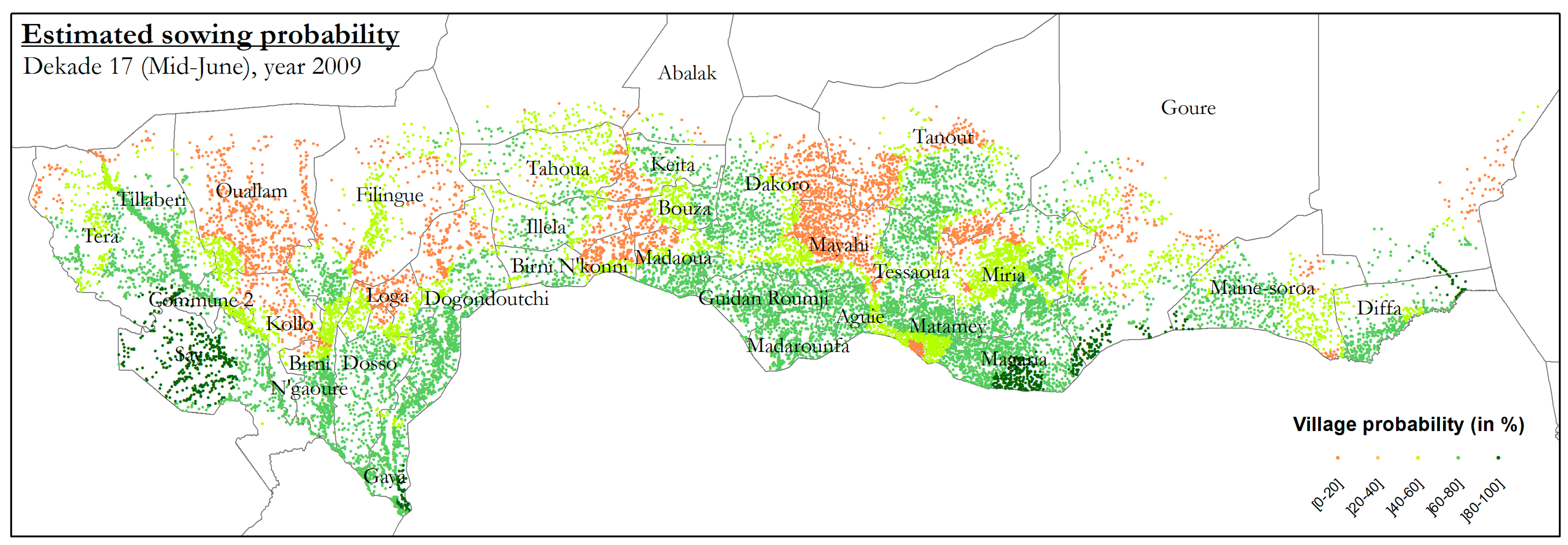
3.3. From Vegetation Onset to Sowing Dates

The relationship between remotely sensed vegetation onsets and the moment of a successful sowing is not trivial. First because of the natural delay of few dekads from the sowing to the first detectable signals of vegetation emergence. Second, at the 250 m scale there is a non-negligible contribution of trees and shrubs on the signal. Note that non-agricultural areas are not excluded from the village buffer mask. However, since the statistical procedure translates percentages of detected pixels into sowing probabilities, no further changes in the methodology would be needed in order to accommodate the exclusion of non-agricultural pixels. The decision to not do so is motivated by the relative unreliability of available crop masks in some regions and by the general principle of parsimony in the modeling procedure. Third, sowing decisions are household specific and may substantially vary within a village. Forth, from the previous point follows that the statement “sowing took (or not) place in a village” relies on undetermined area/household/plot thresholds. The problem of deriving accurately the planting or start-of-the-season dates from satellite imagery remains challenging although the phenological methods have substantially improved [26,34]. However, we believe that the statistical method exposed in Subsection 2.4 is the way to deal with this task. The natural delay is taken into account by testing alternative specifications with lagged detections. It is worth noting that no tested lag is higher than the two dekads that the rainfall-threshold-based method requires before being able to declare that a sowing took place. Consequently, as long as timing is concerned, the tested lags are at worst as good as what one obtains from the rainfall method and at best two dekads sooner. Moreover, in the context of our approach, the contribution of tree and shrubs to the signal may become a solution rather than a problem since they usually react to humidity faster than crops allowing early detections of favorable conditions for successful sowings. Finally, the sowing probabilities derived from the percentage of the pixels around a village where a green-up could be detected can be interpreted as the probability that an agricultural technician asserts an effective sowing in this village given the area, the number of plots or households having sown.

A remaining issue is the fact that the relationship between sowing probabilities and remote sensed vegetation onsets may vary over years. Yearly variations could result from different reactions of natural vegetation (present in mixed pixels) and crops to rainfall temporal distribution and from household sowing strategies. If they are significant, the parameters to be used in the current year are unknown and the model would be unsuitable for operational applications. To test the model stability we cross validate the parameters of one year using the information available for the other year and assess the variations on the performance of the model.

Table 3 summarizes the estimation of the parameters β₀ and β₁ from Equation (2). It shows the relationship between the number of villages having sown at the department level in a given dekad and green-up onsets detected around villages at the same dekad (Lag0) and on the following two dekads (Lag1 and Lag2). Yearly differences have been tested by running the estimation separately for 2008 and 2009. Jackknifed standard deviations of both parameters are also presented. In order to compare the results obtained from the use of vegetation onset detections and the agrometereological approach, two model performance measures are reported: the traditional R-squared and the root mean aggregated squared errors (RMASE) that is defined by Equation (10). The parallelism between the RMASE and the root mean square error (RMSE) is straightforward. In order to get a national level measure, in the RMASE formula the sum of squared errors is divided only by the number of dekads before being square-rooted, while in the RMSE the sum of squared errors is divided by both the number of dekads and the number of departments:

$$RMASE=\sqrt{\frac{1}{T}{\displaystyle \sum _{k=1}^d{\displaystyle \sum _{t=1}^T{(Y_{k,t}-{\widehat{Y}}_{k,t})}^2}}}$$

(10)

where T is the number of dekads (12 in our study case), d is the number of departments (34) and Y_k,t and Ŷ_k,t respectively are the actual and the estimated number of villages having sown in department k at or before dekad t.

Results show that the vegetation onset detection outperforms the rainfall-based approach for all tested lags and on the two considered years. R-squared jumps from 0.74 to [0.81–0.82] in 2008 and from 0.73 to [0.79–0.86] in 2009 meaning a relative improvement from the RFE methodology ranging from 8.22% for Lag2 to 17.81% for Lag0, both in 2009. Higher improvements are observed on the RMASE. It decreases 17.23% when detections 2 dekads lags are used in 2009 and 29.01% with no time-lag for the same year. At this point, it is worth mentioning the parsimony of the statistical approach. The results are obtained with the estimation of only two parameters for the whole Niger and may be improved with no over-fitting issues with the stratification of the villages in two or three groups (estimation of 4 or 6 parameters). Figure 4 shows two scatter plots of the actual number of villages having sown per dekad and department and the model’s predictions for the Lag0 specification in 2008 and 2009.

Table 3. Estimation of the number of villages having sown per dekad and department based on green-up onset detection (Lag columns) versus rainfall method (RFE) for 2008 and 2009. Statistics followed by “cross” refer to predictions for one year based on the parameters estimated for the other year.

Parameter	2008				2009
	Lag0	Lag1	Lag2	RFE	Lag0	Lag1	Lag2	RFE
β0	0.9106	0.6286	0.3836	-	1.2020	1.0316	0.7223	-
sd(β0)	0.0280	0.0088	0.0057	-	0.0836	0.0394	0.0050	-
β1	0.2721	0.2375	0.2640	-	0.3787	0.4173	0.4246	-
sd(β1)	0.0129	0.0030	0.0159	-	0.0260	0.0134	0.0030	-
R2	0.82	0.82	0.81	0.74	0.86	0.83	0.79	0.73
RMASE	869	860	876	1112	783	827	917	1132
R2-cross	0.82	0.82	0.81	-	0.85	0.81	0.77	-
RMASE-cross	860	867	884	-	831	913	1023	-

Table 3. Estimation of the number of villages having sown per dekad and department based on green-up onset detection (Lag columns) versus rainfall method (RFE) for 2008 and 2009. Statistics followed by “cross” refer to predictions for one year based on the parameters estimated for the other year.

Parameter	2008				2009
	Lag0	Lag1	Lag2	RFE	Lag0	Lag1	Lag2	RFE
β0	0.9106	0.6286	0.3836	-	1.2020	1.0316	0.7223	-
sd(β0)	0.0280	0.0088	0.0057	-	0.0836	0.0394	0.0050	-
β1	0.2721	0.2375	0.2640	-	0.3787	0.4173	0.4246	-
sd(β1)	0.0129	0.0030	0.0159	-	0.0260	0.0134	0.0030	-
R2	0.82	0.82	0.81	0.74	0.86	0.83	0.79	0.73
RMASE	869	860	876	1112	783	827	917	1132
R2-cross	0.82	0.82	0.81	-	0.85	0.81	0.77	-
RMASE-cross	860	867	884	-	831	913	1023	-

Figure 4. Actual versus predicted (Lag0 specification) number of villages having sown by department and by dekad. Points’ size are proportional to the total number of villages within a department and months are in shades of green. Number of observations: 34 departments multiplied by 12 periods equals 408 observations for each year.

Figure 4. Actual versus predicted (Lag0 specification) number of villages having sown by department and by dekad. Points’ size are proportional to the total number of villages within a department and months are in shades of green. Number of observations: 34 departments multiplied by 12 periods equals 408 observations for each year.

Both the intercept and the slope are statistically different from zero for all tested specifications. More importantly, the results reject several functional forms between probability of sowing and the fraction of vegetated pixel. First, linear, strictly concave and strictly convex forms are unlikely since β₁ is significantly different from 1. Second, low estimated values of β₁ discard threshold forms. Third, functional forms with change in concavity from concave upward to concave downward can be excluded by the fact that, given the data, β₁ is likely to be smaller than 1. The model consistently selects, for all tested lags and both years, a functional form that changes concavity from downward to upward (Figure 5). The meaning of this robust result is that a sowing is likely to have occurred at the very first signs of vegetation onset. In the Lag0 specification for 2008, there is a 60% probability (62% for 2009) for a sowing to be declared in a village if green-ups are detected in 1% of the pixels. As expected, these probabilities are lower, but still high, for the Lag2 specification: 41% for 2008 and 40% for 2009. From this point on, the probability of sowing increases at a slower pace to reach 82% and 88% (Lag0; 2008 and 2009 respectively) and 65% and 76% (Lag2; 2008 and 2009 respectively) for a green-up detected in 50% of the pixels. Interesting enough, note that the higher is the lag and the more detected pixels are needed for the same sowing probability.

Figure 5. Probability of sowing at the village level as a function of the percentage of pixels within a 5 km buffer where a vegetation onset has been detected, for the three tested lags and 2 years of data. The color surface reproduces the estimated variability (95% confidence intervals) of β₀ and β₁.

Figure 5. Probability of sowing at the village level as a function of the percentage of pixels within a 5 km buffer where a vegetation onset has been detected, for the three tested lags and 2 years of data. The color surface reproduces the estimated variability (95% confidence intervals) of β₀ and β₁.

An important point of concern is that, for the 3 lags, the parameters are significantly different between the two years. As discussed, this raises the issue of the suitability of the method for early warning in years where the parameters are unknown. In order to measure the impact of this difference on the prediction power of the model, results have been cross-validated for each year using the parameters estimated for the other one. The last two rows of Table 3 show cross-validated R-squares and RMASEs. Variations of the overall model performance are small enough to be neglected for 2008 predictions using parameters estimated for 2009. From the other way round, even if a performance decrease of higher magnitude is observed, the model based on green-up onset detection still outperforms the approach based on rainfall thresholds. This being said, the inter-annual parameter variability should be further explored by including new years of data.

Sowing probabilities at the village level can then be periodically (every dekad) produced by replacing the percentage of pixels in the buffer surrounding each village (V_i,k,t) in Equation (2), after Equation (3) conversion. Figure 6 shows an example where villages in the rainfed agricultural and agro-pastoral zones are depicted with their associated sowing probabilities for the 17th dekad of 2009.

Figure 6. Estimated sowing probabilities at the village level for the 17th dekad of 2009 from the 2009 model with Lag0 and 20 pixels buffer.

Figure 6. Estimated sowing probabilities at the village level for the 17th dekad of 2009 from the 2009 model with Lag0 and 20 pixels buffer.

4. Conclusions

To better monitor the start of the crop season in Sahel and provide decision makers with valuable information for an early assessment of yearly crop production, this study proposes an innovative approach that derives sowing probabilities at the village level from satellite imagery. The approach sequentially deals with three issues that cripple the use of vegetation indices for the estimation of sowing dates. First, in order to overcome the limitations in deriving green-up onset dates from remotely sensed vegetation indices, this study relies on a multi-spectral image analysis originally designed for the monitoring of the desert locust habitat. The method guarantees an early, robust and reliable discrimination between vegetated and non-vegetated surfaces, in accordance with the needs for the detection of sowings in Sahel. Second, in order to avoid over-parameterization of the system, the buffer through which green-up detections are associated to a given village is defined a priori such as to include most of the cropped land around the village without including non-cultivated land farther from the village. Third, an original and sound theoretical statistical framework bridges the gap between vegetation onset detections around villages and sowing probabilities. Its strength relies on the fact that the estimation of the parameters is possible with the information on the villages having sown even if aggregated over administrative units, as usually is the case in the Sahelian countries.

Cross-validated results show that by the estimation of only two parameters for the whole country the model outperforms, both in terms of accuracy (RMASE) and in terms of timing, the method based on rainfall thresholds which is presently used to monitor the agricultural season in Sahel.

This study opens new possibilities for the use of satellite remote sensing data for food security monitoring in the region. In operational terms, it has the advantage of providing information early in the season compared to other phenology-based methods that need longer periods of observations to derive the start-of-season dates. However, further experiments should test the methodology for a lager set of years and other countries in the Sub-Saharan window. Finally, other approaches to detect the green-up onset should be investigated in order to improve the performance of predicting sowing dates.

References

1. Sivakumar, M.V.K. Predicting rainy season potential from the onset of rains in Southern Sahelian and Sudanian climatic zones of West Africa. Agric. For. Meteorol. 1988, 42, 295–305. [Google Scholar]
2. Sivakumar, M.V.K. Exploiting rainy season potential from the onset of rains in the Sahelian zone of West Africa. Agric. For. Meteorol. 1990, 51, 321–332. [Google Scholar]
3. Akponikpe, P.B.I. Millet Response to Water and Soil Fertility Management in the Sahelian Niger: Experiments and Modeling. Available online: http://dial.academielouvain.be/downloader/downloader.py?pid=boreal:19624&datastream=PDF_01 (accessed on 3 June 2014).
4. Bacci, L.; Cantini, C.; Pierini, F.; Maracchi, G.; Reyniers, F.N. Effects of sowing date and nitrogen fertilization on growth, development and yield of a short day cultivar of millet (Pennisetum glaucum L.) in Mali. Eur. J. Agron. 1999, 10, 9–21. [Google Scholar]
5. De Beurs, K.M.; Henebry, G.M. Spatio-Temporal statistical methods for modelling land surface phenology. In Phenological Research; Hudson, I.L., Keatley, M.R., Eds.; Springer Netherlands: Berlin, Germany, 2010; pp. 177–208. [Google Scholar]
6. AGRHYMET. Méthodologie De Suivi Des Zones À Risque; AGRHYMET FLASH, Bulletin de Suivi de la Campagne Agricole au Sahel, Centre Regional AGRHYMET: Niamey, Niger, 1996; Volume 2, No. 0/96. [Google Scholar]
7. Graef, F.; Haigis, J. Spatial and temporal rainfall variability in the Sahel and its effects on farmers’ management strategies. J. Arid Environ. 2001, 48, 221–231. [Google Scholar]
8. Dinku, T.; Chidzambwa, S.; Ceccato, P.; Connor, S.J.; Ropelewski, C.F. Validation of high-resolution satellite rainfall products over complex terrain. Int. J. Remote Sens. 2008, 29, 4097–4110. [Google Scholar]
9. Dinku, T.; Ceccato, P.; Cressman, K.; Connor, S.J. Evaluating detection skills of satellite rainfall estimates over desert locust recession regions. J. Appl. Meteorol. Climatol. 2010, 49, 1322–1332. [Google Scholar]
10. Dinku, T.; Ceccato, P.; Connor, S.J. Challenges of satellite rainfall estimation over mountainous and arid parts of east Africa. Int. J. Remote Sens. 2011, 32, 5965–5979. [Google Scholar]
11. Holben, B.N. Characteristics of maximum-value composite images from temporal AVHRR data. Int. J. Remote Sens. 1986, 7, 1417–1434. [Google Scholar]
12. Lillesaeter, O. Spectral reflectance of partly transmitting leaves: Laboratory measurements and mathematical modeling. Remote Sens. Environ. 1982, 12, 247–254. [Google Scholar]
13. Huete, A.R. Soil influence in remote sensed vegetation-canopy spectra. In Introduction to the Physics and Techniques of Remote Sensing; Wiley-Interscience: New York, NY, USA, 1987; pp. 107–141. [Google Scholar]
14. Gutman, G.G. On the use of long-term global data of land reflectances and vegetation indices derived from the advanced very high resolution radiometer. J. Geophys. Res. Atmos. 1999, 104, 6241–6255. [Google Scholar]
15. Despland, E.; Rosenberg, J.; Simpson, S.J. Landscape structure and locust swarming: A satellite’s eye view. Ecography 2004, 27, 381–391. [Google Scholar]
16. Ceccato, P.N. Operational early warning system using SPOT-VGT and TERRA-MODIS to predict desert locust outbreaks. In Proceedings of the 2nd VEGETATION International Users Conference: 1998–2004: 6 Years of Operational Activities; European Commission: Brussels, Belgium, 2005; pp. 65–76. [Google Scholar]
17. Moulin, S.; Kergoat, L.; Viovy, N.; Dedieu, G. Global-Scale assessment of vegetation phenology using NOAA/AVHRR satellite measurements. J. Climate 1997, 10, 1154–1170. [Google Scholar]
18. Tateishi, R.; Ebata, M. Analysis of phenological change patterns using 1982–2000 Advanced Very High Resolution Radiometer (AVHRR) data. Int. J. Remote Sens. 2004, 25, 2287–2300. [Google Scholar]
19. Piao, S.; Fang, J.; Zhou, L.; Ciais, P.; Zhu, B. Variations in satellite-derived phenology in China’s temperate vegetation. Glob. Change Biol. 2006, 12, 672–685. [Google Scholar]
20. Ceccato, P.; Gobron, N.; Flasse, S.; Pinty, B.; Tarantola, S. Designing a spectral index to estimate vegetation water content from remote sensing data: Part 1: Theoretical approach. Remote Sens. Environ. 2002, 82, 188–197. [Google Scholar]
21. Pekel, J.-F.; Ceccato, P.; Vancutsem, C.; Cressman, K.; Vanbogaert, E.; Defourny, P. Development and application of multi-temporal colorimetric transformation to monitor vegetation in the desert locust habitat. IEEE J. Sel. Top. Appl. Earth Obs. Remote Sens. 2011, 4, 318–326. [Google Scholar]
22. Brown, M.E.; de Beurs, K.M. Evaluation of multi-sensor semi-arid crop season parameters based on NDVI and rainfall. Remote Sens. Environ. 2008, 112, 2261–2271. [Google Scholar]
23. Vintrou, E.; Bégué, A.; Baron, C.; Saad, A.; Lo Seen, D.; Traoré, S.B. A comparative study on satellite- and model-based crop phenology in West Africa. Remote Sens. 2014, 6, 1367–1389. [Google Scholar]
24. Funk, C.; Budde, M.E. Phenologically-tuned MODIS NDVI-based production anomaly estimates for Zimbabwe. Remote Sens. Environ. 2009, 113, 115–125. [Google Scholar]
25. Atzberger, C.; Klisch, A.; Mattiuzzi, M.; Vuolo, F. Phenological metrics derived over the european continent from NDVI3G data and MODIS time series. Remote Sens. 2013, 6, 257–284. [Google Scholar]
26. Meroni, M.; Verstraete, M.M.; Rembold, F.; Urbano, F.; Kayitakire, F. A phenology-based method to derive biomass production anomalies for food security monitoring in the Horn of Africa. Int. J. Remote Sens. 2014, 35, 2472–2492. [Google Scholar]
27. Sakamoto, T.; Yokozawa, M.; Toritani, H.; Shibayama, M.; Ishitsuka, N.; Ohno, H. A crop phenology detection method using time-series MODIS data. Remote Sens. Environ. 2005, 96, 366–374. [Google Scholar]
28. Zhang, X.; Friedl, M.A.; Schaaf, C.B.; Strahler, A.H.; Hodges, J.C.F.; Gao, F.; Reed, B.C.; Huete, A. Monitoring vegetation phenology using MODIS. Remote Sens. Environ. 2003, 84, 471–475. [Google Scholar]
29. Xie, P.; Arkin, P.A. Global precipitation: A 17-year monthly analysis based on gauge observations, satellite estimates, and numerical model outputs. Bull. Am. Meteorol. Soc. 1997, 78, 2539–2558. [Google Scholar]
30. Direction Des Statistiques. In Evaluation de la Campagne Agricole 2008/2009 et Résultats Définitifs; Direction Des Statistiques, Ministere Du Developpement Agricole: Niamey, Niger, 2009.
31. Vancutsem, C.; Marinho, E.; Kayitakire, F.; See, L.; Fritz, S. Harmonizing and combining existing land cover/land use datasets for cropland area monitoring at the African Continental Scale. Remote Sens. 2013, 5, 19–41. [Google Scholar]
32. Vancutsem, C.; Pekel, J.-F.; Bogaert, P.; Defourny, P. Mean compositing, an alternative strategy for producing temporal syntheses. Concepts and performance assessment for SPOT VEGETATION time series. Int. J. Remote Sens. 2007, 28, 5123–5141. [Google Scholar]
33. Wang, Y.H. On the number of successes in independent trials. Stat. Sin. 1993, 3, 295–312. [Google Scholar]
34. Meroni, M.; Fasbender, D.; Kayitakire, F.; Pini, G.; Rembold, F.; Urbano, F.; Verstraete, M.M. Early detection of biomass production deficit hot-spots in semi-arid environment using FAPAR time series and a probabilistic approach. Remote Sens. Environ. 2014, 142, 57–68. [Google Scholar]