Improved Surface Reflectance from Remote Sensing Data with Sub-Pixel Topographic Information

Abstract

Several methods currently exist to efficiently correct topographic effects on the radiance measured by satellites. Most of those methods use topographic information and satellite data at the same spatial resolution. In this study, the 30 m spatial resolution data of the Digital Elevation Model (DEM) from ASTER (Advanced Spaceborne Thermal Emission and Reflection Radiometer) are used to account for those topographic effects when retrieving land surface reflectance from satellite data at lower spatial resolution (e.g., 1 km). The methodology integrates the effects of sub-pixel topography on the estimation of the total irradiance received at the surface considering direct, diffuse and terrain irradiance. The corrected total irradiance is then used to compute the topographically corrected surface reflectance. The proposed method has been developed to be applied on various kilometric pixel size satellite data. In this study, it was tested and validated with synthetic Landsat data aggregated at 1 km. The results obtained after a sub-pixel topographic correction are compared with the ones obtained after a pixel level topographic correction and show that in rough terrain, the sub-pixel topography correction method provides better results even if it tends to slightly overestimate the retrieved land surface reflectance in some cases.

1. Introduction

The apparent surface radiance distribution measured from space differs from its intrinsic value on the ground because of the presence of the atmosphere and the influence of topography. Appropriate correction of these atmospheric and topographic effects can improve the retrieved ground objects information and can also be very beneficial for the detection of true changes in the spectral characteristics of the ground cover in multitemporal images use for monitoring purposes [1]. The atmospheric effects on the radiance measured by satellites and methods to correct them have been analyzed and developed for several years and by many authors [2,3,4,5,6].

Thanks to the increasing availability of terrain elevation data, several authors [7,8,9,10,11,12,13] have estimated the effects induced by topography on satellite measured radiometric data. They highlighted that terrain induces variations of the illumination which introduce distortions in the observed radiance and thus also in the estimation of surface properties. Different methods have been developed to account for the impact of illumination at a pixel level and some have been proven efficient to improve the accuracy of retrieval of surface radiance [14,15,16].

In past years, more accurate digital elevation models (DEM) became available at a global scale with a resolution of up to 30 m. On the other hand, currently used geostationary satellites provide data in the solar domain at the kilometric level. The availability of higher resolution DEM enables us to consider terrain effects on the measured radiance at a finer resolution allowing the exploration of the effects of topography at a sub-pixel level. Some studies [17,18,19,20] explored the effects of sub-pixel heterogeneity on the retrieved surface properties. So far, most of these studies focused on land cover heterogeneity within a pixel and few started to look into sub-pixel topography variability. From the latter, it appeared that in rugged terrain, neglecting the sub-pixel terrain variability surface properties derived at different spatial resolutions can appear considerably different even though using the same model [18], highlighting the necessity to account for these sub-pixel effects.

The issue was tackled by Wen [19] who described the sub-pixel topographic effects on the surface albedo estimation and developed a correction factor. This study illustrated the necessity of sub-pixel topographic correction in rugged areas and showed promising results. However, it did not consider all the effects of topography, such as the pixel adjacency effect which was neglected although it has been proven as having a high influence on satellite measured radiance in rugged areas. The study presented in this article aims at developing an operational method to correct sub-pixel topography induced effects on measured kilometric pixel size satellite data using a fine resolution DEM and integrating the sub-pixel adjacency effect. This method can be applied on different spatial resolution combinations but is tested and validated here using Landsat data aggregated at 1 km resolution to simulate coarser satellite data along with the 30 m DEM from ASTER-GDEM2. Those data were measured over the southern part of the Tibetan Plateau, chosen for its extreme terrain relief. In Section 2, the topographic dataset, the topography of the plateau and the study site are described. Section 3 provides a short theoretical background on topographic correction followed by the description of the sub-pixel topography correction method. More detailed descriptions of the main sub-pixel topographic correction parameters are given in Section 4. Then, the main results and conclusions are presented in Section 5 and Section 6, respectively.

2. Site and Data Description

2.1. Topographic Data

The characteristics of the topography are retrieved at 30 m resolution from the DEM provided by the Advanced Spaceborne Thermal Emission and Reflection Radiometer (ASTER), i.e. the Global Digital Elevation Model (GDEM) version 2. ASTER-GDEM2 is one of the most complete high-resolution digital topographic dataset in the world to date. The ASTER-GDEM2 covers land surfaces between 83°N and 83°S at a spatial resolution of 1 arc-second. Even if some geolocalisation errors and elevation aberrations have been identified at the global scale, this dataset remains the best alternative in accessibility to high-quality elevation data for the selected study site [21].

2.2. Tibetan Plateau

The Tibetan Plateau, a geological structure lying between the Himalayan range to the south and the Taklimakan desert to the north (Figure 1), is the largest and highest plateau area in the world spreading over 1.2 million km² and presenting an average elevation of over 5000 meters. The plateau is also characterized by a very high spatial heterogeneity due to the presence of mountainous areas affecting radiance measurements over space and time. It is, therefore, an ideal study region to test the sub-pixel topographic method developed in this article as the surface radiance measured from space cannot be accurately estimated in this area without taking into consideration the effects of topography. To conduct this study, a test area with increasing effect of topography (right part of Figure 1), starting from relatively flat, then hilly landscape, and finally complex relief is identified from the DEM.

Figure 1. The Tibetan Plateau and the study site used to test the sub-pixel topographic correction.

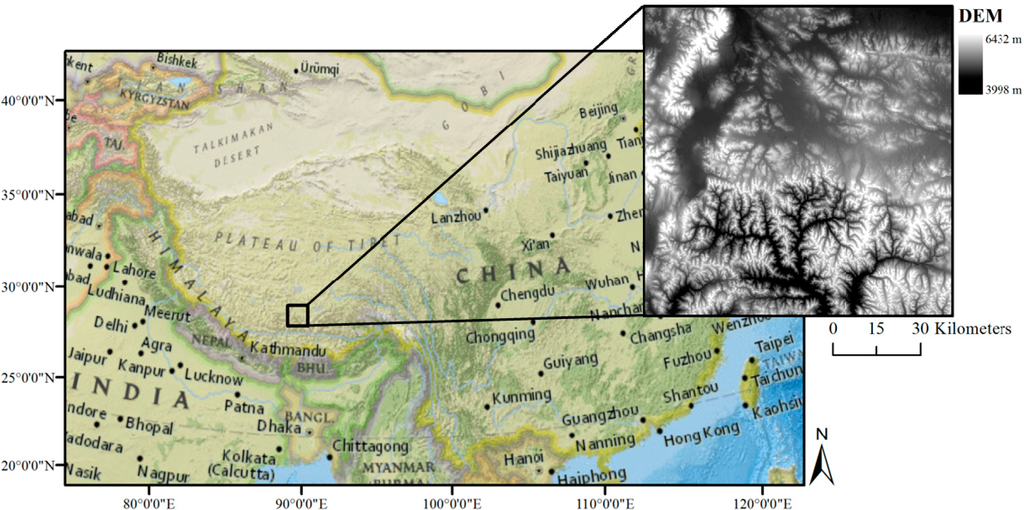
Figure 1. The Tibetan Plateau and the study site used to test the sub-pixel topographic correction.

It is essential to characterize the topography of the area prior to quantifying its effects on surface radiance measurements from space. To this end, the slope and aspect, two key topographic parameters, have been derived from the DEM at a resolution of 30 m. By summarizing the distribution of the slope values over the entire plateau in a frequency plot, Figure 2a shows that more than 25% of the plateau is covered by terrain with a slope value over of 20°. Focusing on the site area, Figure 2b shows a rougher terrain with an important density of slope between 5° and 35°. In that area, about 40% of the terrain presents a slope steeper than 20°.

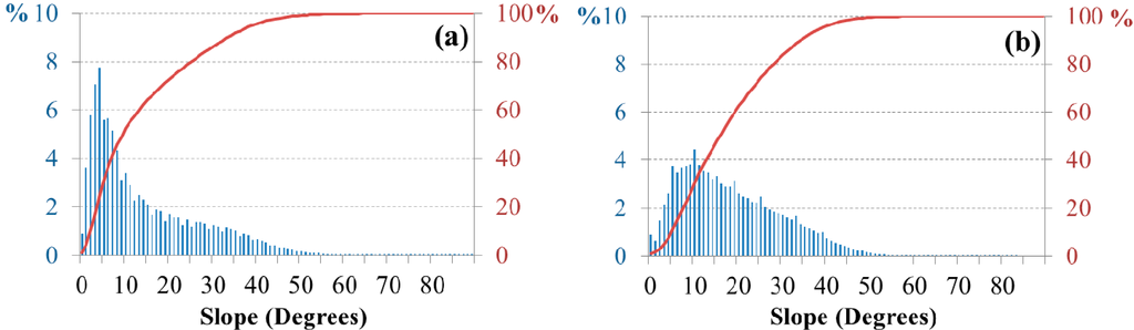
Figure 2. Slope values distribution over the Tibetan Plateau (a) and the study area (b), expressed as percentage per slope gradient (histogram) and cumulated percentage (red line).

Figure 2. Slope values distribution over the Tibetan Plateau (a) and the study area (b), expressed as percentage per slope gradient (histogram) and cumulated percentage (red line).

2.3. Sub-Pixel Heterogeneity

Before to continue with the analysis, it is important to clearly define the concept of pixel and sub-pixel level as it is the basis of this study. In this paper, the 30 m spatial resolution DEM is considered as the sub-pixel level and the kilometric pixel size satellite data as the pixel level. Figure 3 shows a theoretical scheme illustrating this concept of sub-pixel and pixel level.

Figure 3. Sub-pixel and pixel level concept (the greyscale represents theoretical radiance values).

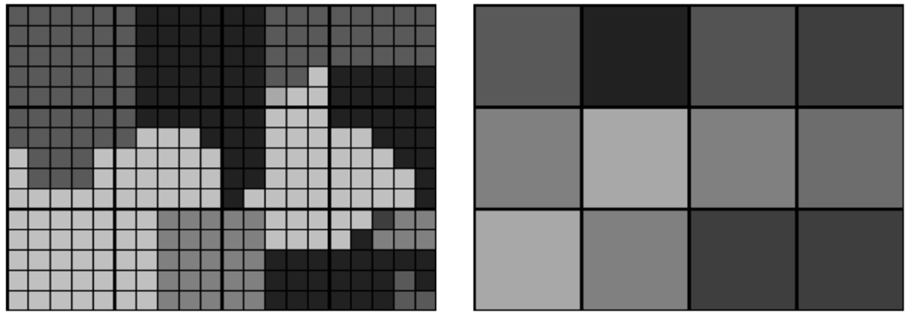
Figure 3. Sub-pixel and pixel level concept (the greyscale represents theoretical radiance values).

As the main topic of this study is the sub-pixel topography effects (Figure 3), the distribution of slope and aspect values at 30 m resolution within each square kilometer pixel have been analyzed. To do so, two statistical parameters, skewness and kurtosis, which express the symmetry and shape of the distributions respectively, are used to describe the sub-pixel topography. Those parameters allow to classify the topography distribution within a kilometer resolution pixel as “normal” if the skewness equals zero and the kurtosis equals three (with a tolerance ranging from minus to plus twice the standard error of skewness and kurtosis respectively [22]), as “maybe normal” if only one of the two parameters indicates a normal distribution and as “not normal” if none of the two parameters indicates a normal distribution. The results are displayed in Figure 4, where the normality distribution within each 1 km pixel for the terrain aspect is presented on the left and for the slope on the right. Those results illustrate that the sub-pixel distribution of slope and aspect values within each kilometric pixel is mostly not normal, which highlights the necessity to account for this sub-pixel topography because the averaged slope and aspect values at a pixel level would mask out the real effects of topography on the measured radiance.

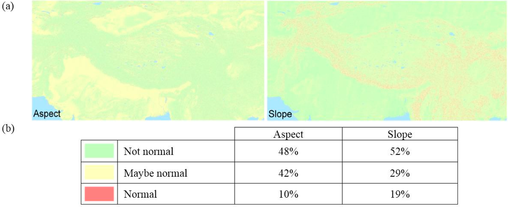
Figure 4. Slope and aspect sub-pixel normality distribution maps (a) and statistics (b) within each square kilometer pixel over the Tibetan Plateau and the surroundings.

Figure 4. Slope and aspect sub-pixel normality distribution maps (a) and statistics (b) within each square kilometer pixel over the Tibetan Plateau and the surroundings.

3. Topographic Correction

3.1. Topographic Correction at Pixel Level

In a remote sensing context, radiance is what is measured at the sensor and corresponds to the brightness in a given direction toward the sensor. Surface radiance is often converted to surface reflectance, the ratio of reflected versus total radiant energy, prior to further data analysis.

The reflected radiance measured by a geostationary satellite consists of the path radiance (L_p), which does not interact with the surface but is scattered back to the sensor by the atmosphere, and the radiance reflected by the Earth surface to the sensor (L_s), which has a complex interaction at the Earth surface and atmosphere boundary. After correcting the top-of-atmosphere radiance measured by the satellite for atmosphere effects using an atmospheric radiative transfer model such as MODTRAN, L_s is obtained but still needs to be corrected for topographic effects. L_s is converted in surface reflectance (ρ) according to Equation 1, which assumes that the surface target is a Lambertian reflector.

$$\rho =\pi \times \frac{L_s}{E}$$

(1)

In Equation (1), L_s represents the reflected surface radiance (W/sr/m²) measured by the geostationary satellite and E is the total solar irradiance (W/m²) at the surface.

The topographic correction presented in Sandmeier [23] is quoted and applied in several studies [13,24,25,26] to correct the relief induced distortions on satellite measured data at a pixel level. This topographic correction is based on the fact that, in order to account for the topographic effects, the total solar irradiance variable in Equation (1) should be corrected according to the effects induced by the relief. In this method, E is divided into three components: direct irradiance (E_d), diffuse irradiance (E_f) split into two components, the isotropic and the circumsolar diffuse irradiance, and the terrain irradiance (E_t). The equation to estimate the corrected total solar irradiance assumes the surface as Lambertian and is expressed as [23]:

$$\begin{gathered} E =\Theta \times E_d\times \frac{cos{\theta }_i}{cos{\theta }_s}+E_f\times \left[k\times \frac{cos{\theta }_i}{cos{\theta }_s}+\left(1-k\right)\times V_d\right]+E_t \\ =\Theta \times E_d\times \frac{cos{\theta }_i}{cos{\theta }_s}+E_f \times \left[k\times \frac{cos{\theta }_i}{cos{\theta }_s}+\left(1-k\right)\times V_d\right]+\left(E_d+E_f\right)\times V_t\times {\rho }_{adj} \end{gathered}$$

(2)

In Equation (2), Θ is the binary coefficient to control cast shadow, θ_i is the angle of sun’s incidence (rad) and θ_s is the solar zenith angle (rad), k is the anisotropy index, V_d and V_t are the sky-view and terrain-view factor respectively and ρ_adj is the average reflectance of adjacent objects. The first term of Equation (2) shows the cosine law [10] applied to E_d on a horizontal surface and results in the amount of direct irradiance on a tilted target. The irradiance parameters E_d, E_f and k can be estimated using MODTRAN (MODerate resolution atmospheric TRANsmittance and radiance).

3.2. Topographic Correction at Sub-Pixel Level

Until now, this topographic correction method has generally been applied using a DEM and satellite data at the same spatial resolution. However, when considering an area with a relief as rugged as the relief of the Tibetan Plateau, using optical data from geostationary satellite at the kilometric level and knowing that higher resolution DEM is available, it is of interest to check the improvement that would be achieved by making use of this higher resolution topographic data. In other words, we aim at evaluating the improvement achieved by carrying out a sub-pixel topographic correction. Referring to sub-pixel correction means to use high resolution data to perform a correction on lower resolution data, while keeping the original resolution of both datasets. In this case, to use a 30 m resolution DEM to topographically correct kilometric level geostationary satellite data instead of degrading the data from the DEM at the kilometric level prior to applying the topographic correction.

In this research, the idea is to apply Equation (2) to each pixel of the 30 m DEM, considered as the sub-pixels of the geostationary radiometric optical data at 1 km spatial resolution. As compared to the initial topographic correction scheme of Sandmeier [23], the novelty of this method lies in the fact that the computation of the total surface irradiance accounting for topographic effects is performed at sub-pixel level preserving the original DEM information. Then the topographically corrected surface irradiance is averaged into a sub-pixel topographically corrected surface irradiance grid at 1 km (E_av).

$${\rho }_{av}=\pi \times \frac{L_s}{E_{av}}$$

(3)

The sub-pixel topographically corrected surface reflectance ρ_av estimated from the reflected surface radiance (L_s) measured by the satellite can be calculated using Equation (3). All the processing steps are summarized in Figure 5.

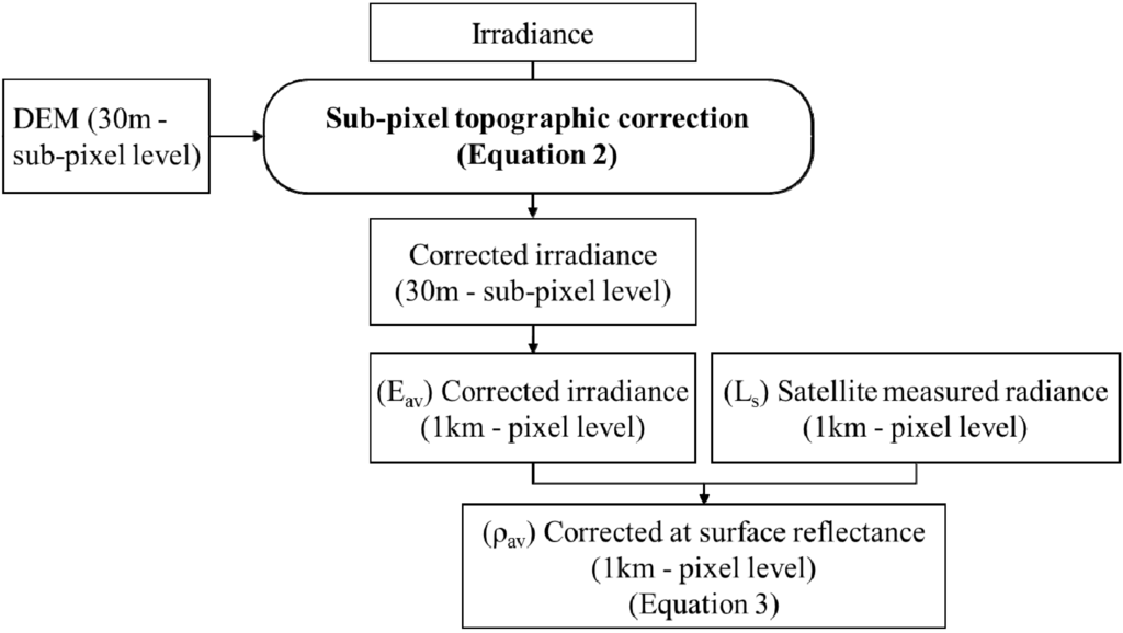
Figure 5. Sub-pixel topographic correction steps.

Figure 5. Sub-pixel topographic correction steps.

3.3. Anisotropy Test

In the presented sub-pixel topographic correction, the sub-pixel anisotropy, also known as non-Lambertian property, is neglected. This means that the surface is considered as reflecting radiance equally into all directions. In reality surfaces are not Lambertian and their anisotropy is characterized by a bidirectional reflectance distribution function (BRDF) which is a four-dimensional function that defines how light is reflected by a surface. The function takes a negative incoming light direction and a positive outgoing direction, both defined with respect to the surface normal by a zenith and an azimuth angle, and returns the ratio of reflected radiance.

In order to quantify the impact of neglecting the sub-pixel non-Lambertian surface property when applying the sub-pixel topographic correction, an anisotropy test is designed. For this test, a theoretical area of 30 by 30 pixels, and therefore 900 possible slope and aspect combinations, is considered. The slope and aspect values come from the ASTER-GDEM2 and are used to compute the sub-pixel corrected irradiance. For a given BRDF function taken from Engelsen [27] and a given solar position, the sub-pixel reflectance is computed using the Rahman-Pinty-Verstraete (RPV) model [28]. Then two scenarii are run and compared. The first scenario assumes the sub-pixel slope and aspect isotropy, which means that, whatever the solar and observations angles variations at sub-pixel level, a unique reflectance value is defined for all the sub-pixels as if the surface was Lambertian, i.e., reflecting equally in all directions. In this scenario, the reflectance value is retrieved from the BRDF function using the mean illumination and observation angles over the considered area. In the second scenario, the reflectance is retrieved accounting for the anisotropy property, which means that a different reflectance value is set for each sub-pixel according to the illumination and observation angles. The reflectance values obtained from the two scenarios are combined with the sub-pixel corrected irradiance to compute the sub-pixel radiance values. The latter are averaged over the entire area and compared. The first scenario provides an isotropic radiance while the second scenario provides an anisotropic radiance. This experiment is repeated for 10 sites selected over the mountainous part of the plateau, 6 different days and 3 different times for each day. The results are summarized in Figure 6 which presents the correlation between the anisotropic and isotropic radiance values produced by the two scenarios for 5 solar zenith angle classes and 5 different BRDF.

Figure 6 highlights the fact that for zenith angles smaller than 60 degrees, the values of reflectance computed considering the sub-pixel anisotropy are highly correlated with the reflectance values computed assuming the sub-pixel level as being isotropic. Concerning larger solar zenith angles, this correlation is no longer significant. This can be due to the sub-pixel anisotropic property of the surface but also to the model limitations when modeling BRDF at extreme solar angles. Large solar zenith angles can be observed just after sunrise and before sunset but they can also be the consequence of the topographic effects in the rough areas. However, based on the results presented in Figure 6 and the fact that less than 5% of the test area is covered by slopes larger than 40°, the choice is made to assume the sub-pixel surface as isotropic for this study.

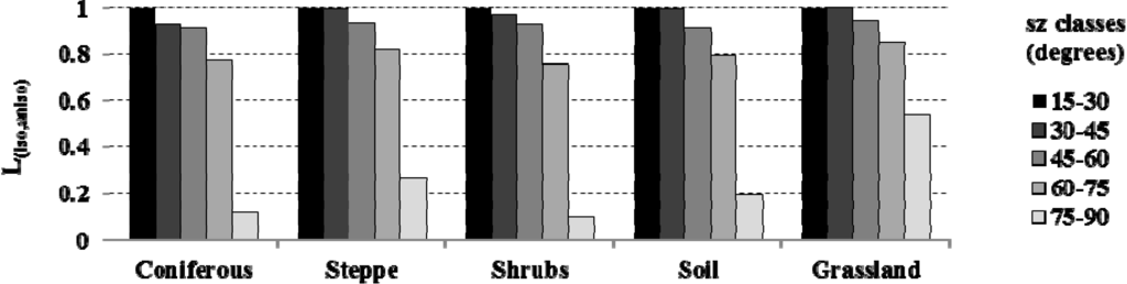
Figure 6. Correlation between anisotropic and isotropic radiance values for 5 solar zenith angle classes and 5 different BRDF.

Figure 6. Correlation between anisotropic and isotropic radiance values for 5 solar zenith angle classes and 5 different BRDF.

4. Sub-Pixel Topographic Correction Parameters

4.1. Shadow Binary Factor

An essential parameter when correcting direct solar irradiance is the binary coefficient Θ used to control cast shadow coming from self-shadowing and shadow from surrounding topography, known as the shadow binary factor (SBF). The value of the SBF depends on the sun’s position at the date and time of data acquisition, which means that it needs to be estimated each time a correction is carried out. To do so, a small module is developed to compute automatically the SBF according to the topography, the day of the year and the local time for each sub-pixel inspired by the methodology presented in Kastendeuch [29].

The aim of this algorithm is to generate a raster at sub-pixel resolution filled with values of 0 or 1. A value of 0 characterizes a pixel in the shadow and a value of 1 characterizes a pixel receiving direct sunlight. In order to compute this SBF, each pixel is tested individually. The first test consists in checking if the pixel itself, without considering the surrounding topography, receives direct light from the sun or not. This is done by comparing the respective solar azimuth and elevation angles with the pixel aspect and slope values. If the pixel is not self-shadowing, then it can be tested for the shadow from surrounding pixels. Using the sun azimuth angle, the pixels located on the path between the sun and the center of the tested pixel are identified. In Figure 7a, the tested pixel is colored in dark grey and the pixels located on the path to the sun are colored in light grey. All the pixels located on the path to the sun could potentially bring shadow to the tested pixel if their elevation is higher than the sun elevation (Figure 7b). As soon as a pixel is identified as shadowing the tested pixel, the test stops, the value of the tested pixel set to 0 and the algorithm starts to test the next pixel. If none of the pixels located on the path to the sun have a larger elevation angle than the sun, then the tested pixel is in the sunlight, its value is set to 1, and the algorithm starts to test the next one.

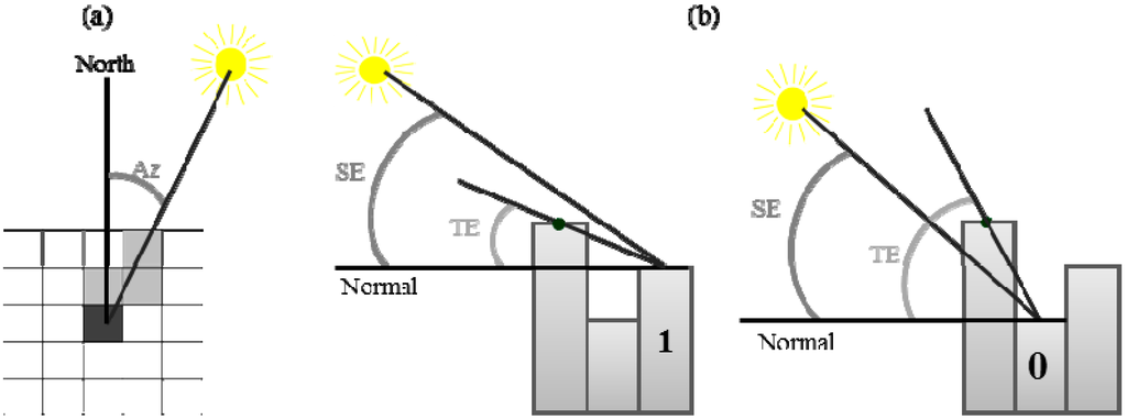
Figure 7. Shadow Binary Factor computation tests (Az = Azimuth angle, SE = Sun elevation angle, TE = Terrain elevation angle). (a) Identification of the pixels located on the path to the sun, (b) Test of shadowing effect of neighboring pixels according to the difference between terrain and sun elevation angles.

Figure 7. Shadow Binary Factor computation tests (Az = Azimuth angle, SE = Sun elevation angle, TE = Terrain elevation angle). (a) Identification of the pixels located on the path to the sun, (b) Test of shadowing effect of neighboring pixels according to the difference between terrain and sun elevation angles.

Figure 8 shows the outputs of the SBF algorithm run for a day time period between 9.00 am and 12.00 pm local time with an increment step of one hour over the study site. This figure highlights the important variations in the amount of shaded areas in one hour time which can represent the time step between two subsequent geostationary satellite data acquisitions. Moreover, the strong relief located in the southern part of the study site shows that a significant amount of pixels remained in the shadow even when around mid-day. Thus, the impact of shaded areas should not be neglected in area characterized with strong relief.

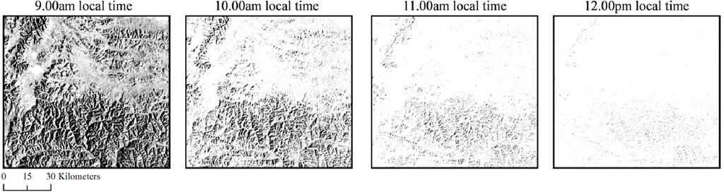
Figure 8. Shadow Binary Factor evolution over day time (shadowed pixels in black and illuminated pixels in white).

Figure 8. Shadow Binary Factor evolution over day time (shadowed pixels in black and illuminated pixels in white).

4.2. Sky View Factor

A view factor is a geometric ratio expressing the fraction of the radiation output from one surface that is intercepted by another [30]. The sky view factor (Vs) accounts for the portion of the overlying hemisphere visible to a grid point. To calculate it, one needs to know the slope and the aspect of the point, as well as the horizon angle in a discrete set of directions [31]. In this study, the sky view factor is computed using the algorithm developed by Zaksek [32], where it is defined by the share of the visible sky above a certain observation point. The algorithm computes vertical elevation angle of the horizon in a user defined number of directions and radius range expressed in pixels. For the purpose of this study, several tests have been carried out to know what would be the best compromise between accuracy and computation time when choosing the number of search directions and radius range to compute the sky-view factor. The two first graphs presented in Figure 9 shows the improvement, expressed as mean difference, achieved: (a) by increasing the radius range for different set of directions and (b) by increasing the number of search directions for different radius ranges. The third graphs (c), shows the computation time required depending on the number of search directions and radius range.

In the Figure 9, the graph (a) shows that, whatever the number of search directions, the difference in Vs values obtained with different radius range reduces significantly between 10 and 30 pixel radius range. Over 30 pixels, the difference due to the increase of radius range is varying less. If one relates this results to the graph (c), showing that when the number of search directions or the radius range increase the computation time increases as well, a radius range of 30 pixels appears as the best compromise in this case. The same reasoning is followed to define the optimum number of search directions. The graph (b) shows that when using a radius range over 10 pixels, the major difference is between using 8 or 16 search directions. Increasing the number of search directions over 16 would only increase the computation time. From the results of these tests, directions and radius have been set to 16 directions and 30 pixels respectively, which is in line with the thresholds given in Dozier [31].

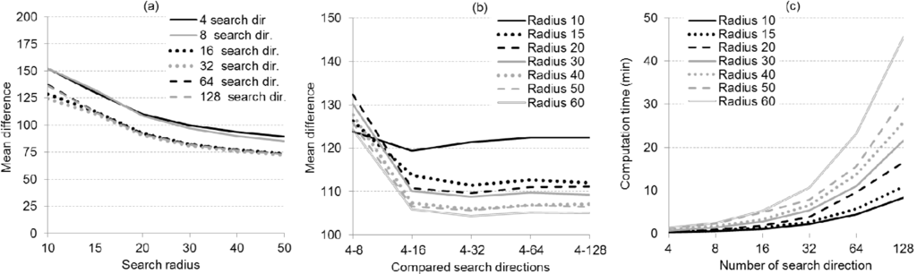
Figure 9. Sky-view factor parameter tests: (a) mean difference according to search radius value for difference search direction, (b) mean difference according to the number of search direction for difference search radius values, (c) computation time required depending on the number of search directions and search radius values.

Figure 9. Sky-view factor parameter tests: (a) mean difference according to search radius value for difference search direction, (b) mean difference according to the number of search direction for difference search radius values, (c) computation time required depending on the number of search directions and search radius values.

5. Results and Discussion

The presented sub-pixel topographic correction method is made of two steps (Figure 5): the computation of sub-pixel corrected surface irradiance (E_av) leading to the estimation of the sub-pixel corrected surface reflectance (ρ_av). For each step, the impact of sub-pixel topography correction is analyzed. To highlight the improvement brought by integrating the sub-pixel topography effects, two levels of topographic correction are computed and compared: (1) a topographic correction at a pixel level, performed using the slope and aspect values degraded from 30 m to 1 km pixel size; (2) a topographic correction at a sub-pixel level, performed using slope and aspect at 30 m.

5.1. Sub-Pixel Topographically Corrected Irradiance

To quantify the impact of sub-pixel topography on the surface irradiance, the latter has been computed according to Equation (2) for different slope and aspect combinations and subtracted to the irradiance value obtained assuming a flat terrain. The slope ranges from 0° to 45° and the relative aspect, i.e., the difference between the solar azimuth angle and the terrain aspect, ranges from 0° to 180°. The computation is performed hourly from 9 am to 6 pm (UTC+8), and the SBF and the sky view factor have been set to 1. The Figure 10a shows hourly maps presenting the irradiance difference (W∙m⁻²) between computation without and with sub-pixel topographic correction. As a summary, the Figure 10b provides the percentage of sub-pixel topographically corrected pixels that are overestimated, underestimated or equal as compared to the irradiance values estimated without topographic correction for each hour of day time.

The objective of this analysis is to highlight the impact of slope and aspect on estimated surface irradiance and to identify if there could be some compensation effects between slope and aspect variations. The graph presented at the bottom of Figure 10 shows that, whatever the time of the day, assuming a flat terrain would not lead to an error in surface irradiance estimation in only 2.17% (green line) of the cases. Thus, in only 2.17% of the tested combinations there is a compensation effect between the slope and aspect values that leads to the same results as if the surface was flat. Moreover, Figure 10 shows that the observed differences are not equally spread between under and over-estimation. Indeed, for the whole range of slope and aspect combinations tested, neglecting the sub-pixel topography mostly leads to an over-estimation of the surface irradiance. The over-estimation is even more important around the solar noon where it represents more than 70% of the cases. The observed errors can reach up to 600 W∙m⁻² or −600 W∙m⁻² in some extreme topographic configurations with strong slope or aspect values, almost leading to a self-shadowing of the pixel. In those cases, there is far less direct illumination as compared to the corresponding flat surface and the irradiance that would be received by a flat surface at solar noon (about 1100 W∙m⁻²) is almost divided by 2. Those results support the observation made in Section 2, concerning the necessity to account for the sub-pixel topography effects because the averaged slope and aspect values at a pixel level would mask out the real effects of topography on the measured radiance. More than the fact that the distribution within kilometric pixel in this area is mostly not normal, the compensation effect that could be expected from a normal distribution of slope and aspect is not confirmed.

Figure 10. Difference between irradiance (W∙m⁻²) computed without and with sub-pixel topographic correction over the day (DOY = 115): (top) Difference maps ranging from −600 (blue) to 600 (red) with the X axis representing the slope gradient and the Y axis the relative aspect, both in degree. (bottom) Irradiance difference summary according to local standard time.

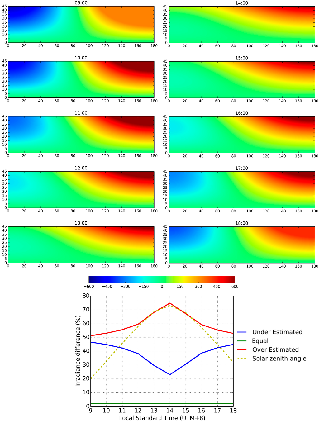
Figure 10. Difference between irradiance (W∙m⁻²) computed without and with sub-pixel topographic correction over the day (DOY = 115): (top) Difference maps ranging from −600 (blue) to 600 (red) with the X axis representing the slope gradient and the Y axis the relative aspect, both in degree. (bottom) Irradiance difference summary according to local standard time.

To further explore the effect of applying a topographic correction at the sub-pixel level when computing surface irradiance, a second test is performed applying Equation (2) over the study site and assuming the reflectance of the adjacent terrain to be equal to 0.2 (arbitrary value representative of the study area). Thus, only the slope and aspect parameters derived from the DEM and available at a sub-pixel level are changing over the scene along with the different view and solar angles used in the computation changing according to the day and time of the day. The irradiance maps are computed each five day of the year and each hour of the day, from 9 am to 6 pm (UTC+8). This time range was chosen because it represents a constant period over the year when the study site is always illuminated. The maps obtained with the pixel level method are subtracted to the corresponding maps obtained with the sub-pixel level method. Then the difference maps are summarized according to the five-number summary method that provides the sample minimum, the first quartile, the median, the third quartile and the sample maximum. From this, the spread of the difference between irradiance computed at pixel and sub-pixel level is derived hourly over the whole year, as presented in Figure 11. The spread of the difference is expressed as the interquartile range, which is the range between the first and the third quartile computed in the five-number summary. The graphs (a) and (b) show this daily interquartile variation over the year for the SBF and for the ratio between solar incidence and solar zenith angle respectively. Concerning the SBF, the difference is expressed as the difference in lighted area (km²). Those two variables have the highest impact in the difference between computing the total irradiance at pixel or at sub-pixel level (Equation (2)). The level of computation of the sky and terrain view factors is also impacting the topographic correction but the difference is fixed over the year. The graphs (c) and (d) show the daily interquartile difference spread over the year for the total irradiance, with real and normalized data respectively. Concerning the direct, diffuse and terrain irradiance variables used in Equation 2, their values vary over the day and the year. However, the values used for those variables are the same in both correction levels. Their values can then influence the shape of the graph but not the difference between the two methods.

Figure 11. Hourly and daily variation of differences between sub-pixel and pixel level corrections for: (a) Shadow binary factor, in km² of lightened area; (b) ratio between incidence and zenith solar angle in radian; (c) Total irradiance values in W∙m⁻²; (d) Total irradiance normalized values in percentage.

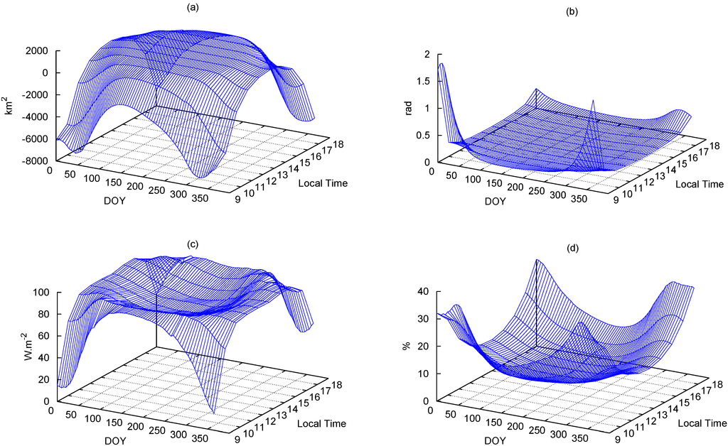
Figure 11. Hourly and daily variation of differences between sub-pixel and pixel level corrections for: (a) Shadow binary factor, in km² of lightened area; (b) ratio between incidence and zenith solar angle in radian; (c) Total irradiance values in W∙m⁻²; (d) Total irradiance normalized values in percentage.

Figure 11 shows that the differences between the two methods depend on the period of the year as well as on the time of the day. Concerning the total irradiance, it is important to make the distinction between the expression of the difference between pixel and sub-pixel level method expressed in W∙m⁻² (graph (c)) and the normalised value (graph (d)) given the difference in percentage. The latter shows that the largest differences between pixel and sub-pixel level topographic correction occur just after sunrise and just before sunset and especially in winter time, when the sun elevation is low. This is explained by the fact that the total irradiance is mainly influence by the direct irradiance which is itself essentially controlled by the SBF. The latter, set to 0 or 1, controls the cast shadow of a pixel which means that it defines if a certain pixel receives direct irradiance or not. From the graph (a) in Figure 11, it appears that the largest differences in lighted area occur during the first and last hours of sunlight. The same observation is made for the ratio between incident and zenith solar angle. The dissymmetry of graph (b) is due to the fact that the computations are run between 9 am and 6 pm, so they are not always centerd on the local solar noon. However, when looking at the difference between the two methods with respect to the total amount of irradiance expressed in W∙m⁻², the largest discrepancies can be observed in the middle of the day and especially in winter time. This is linked to the fact that largest values of direct and diffuse irradiance value are introduced in Equation (2) for this time of the day.

5.2. Sub-Pixel Topographically Corrected Reflectance Retrieved from Aggregated Landsat Data

The previous test highlighted the differences between surface irradiance computed at pixel and sub-pixel level (Figure 11). In order to validate the presented sub-pixel topographic correction quantitatively, a cloud free Landsat-7 (Data available from the U.S. Geological Survey) scene from the 27 October 2007 taken over the Tibetan Plateau is used (Figure 12). The methodology is developed to be used in the solar domain of the spectrum. Thus, only the four first bands as well as the panchromatic band (band 8) of the Landsat image were used. The Landsat data, available at 30 m resolution, can be used as ground truth and the same Landsat data aggregated at 1 km resolution can be considered as radiance values measured by a geostationary satellite. Then, three datasets are produced and compared for the validation: (1) a Landsat data at 30 m corrected using the DEM at the same resolution, which is then aggregated at 1km. This dataset will be considered as the reference data; (2) a Landsat dataset upscaled at 1 km and corrected for topography at pixel level (DEM at 1 km); (3) a Landsat data upscaled at 1 km and corrected for topography at sub-pixel level (DEM at 30 m).

To highlight the improvement brought by integrating the sub-pixel topography effects in the reflectance retrieved at 1 km, the results of pixel level (2) and sub-pixel level (3) topographic correction are respectively compared to the reference map (1). This comparison is performed for the four first bands and the panchromatic band of the selected Landsat scene. The differences obtained for the panchromatic band are presented in Figure 12c while the mean and standard deviation of the differences obtained over the whole scene are summarized in Table 1 for all the processed bands. Figure 12c shows a larger dispersion of the values for the difference between the reference and the pixel level correction while the difference between the reference and the sub-pixel level is more compact and located around zero. This result is the same for the five bands as shown by the statistics in Table 1. Thus, whatever the considered band, the sub-pixel topographic correction method provides more accurate results than the pixel level correction method in all the considered bands even if this method tends to slightly overestimate the retrieved reflectance. This overestimation is the consequence of an underestimation of the surface irradiance. This may be explained by the fact that the correction method applied in this study is using the cosine law to account for topographic effects on direct irradiance estimation (Equation (2)) and several studies showed that this function tends to overestimate the corrected reflectance values [15,16,33]. Even if the proposed correction method also accounts for diffuse and terrain irradiance, the corrected values are still overestimated. However this overestimation remains low and concerns less than 30% of the pixels and is mostly under 0.03. In contrast, the pixel level correction tends to overestimate the surface reflectance for more than 60% of the pixels and this error can reach 0.05.

Figure 12. (a) Study site DEM, (b) Corresponding Landsat-7 scene and (c) Difference between reference reflectance and pixel (top) or sub-pixel (bottom) topographically corrected reflectance for the band 8 of Landsat-7.

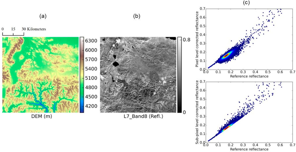
Figure 12. (a) Study site DEM, (b) Corresponding Landsat-7 scene and (c) Difference between reference reflectance and pixel (top) or sub-pixel (bottom) topographically corrected reflectance for the band 8 of Landsat-7.

Table 1. Difference mean and standard between the reference reflectance and pixel (left) or sub-pixel (right) topographically corrected reflectance for Landat-7 band 1, 2, 3, 4 and 8.

	Pixel Level Mean	Pixel Level Standard Deviation	Sub-Pixel Level Mean	Sub-Pixel Level Standard Deviation
Band 1	0.007	0.012	−0.001	0.008
Band 2	0.007	0.013	−0.002	0.010
Band 3	0.007	0.015	−0.003	0.010
Band 4	0.007	0.017	−0.004	0.011
Band 8	0.007	0.016	−0.003	0.012

Table 1. Difference mean and standard between the reference reflectance and pixel (left) or sub-pixel (right) topographically corrected reflectance for Landat-7 band 1, 2, 3, 4 and 8.

	Pixel Level Mean	Pixel Level Standard Deviation	Sub-Pixel Level Mean	Sub-Pixel Level Standard Deviation
Band 1	0.007	0.012	−0.001	0.008
Band 2	0.007	0.013	−0.002	0.010
Band 3	0.007	0.015	−0.003	0.010
Band 4	0.007	0.017	−0.004	0.011
Band 8	0.007	0.016	−0.003	0.012

Furthermore, to quantify the impact of sub-pixel topography on reflectance retrieved from the Landsat-7 image aggregated at 1 km resolution, the standard reflectance product computed without accounting for topography is compared to the sub-pixel topographically corrected reflectance. Figure 13a shows the reflectance difference obtained when subtracting the sub-pixel corrected reflectance map from the uncorrected reflectance map. Along with the histogram (Figure 13b), it shows that the sub-pixel corrected reflectance values are mostly higher than the uncorrected ones. This means that the surface reflectance is underestimated, then that the total irradiance is overestimated, when the sub-pixel topography effects are not considered. This result is logical as no shadow effect is integrated when neglecting sub-pixel topography effects. The Landsat-7 image used was recorded on the 27 October at 10.40 am (local solar time) with a sun elevation angle of 42.5 degrees. The scene (Figure 13a) is then illuminated from the lower right corner, and the only pixels where the reflectance values are higher without sub-pixel topographic correction are the pixel with a slope facing the sun. In this case, assuming a flat terrain led to an underestimation of the received irradiance and thus an overestimation of the reflectance.

Figure 13. (a) Maps of the differences between reflectance values estimated from Landsat-7 band 8 with sub-pixel topographic reflectance as compared to the uncorrected reflectance value, (b) graph summarizing the distribution of those differences.

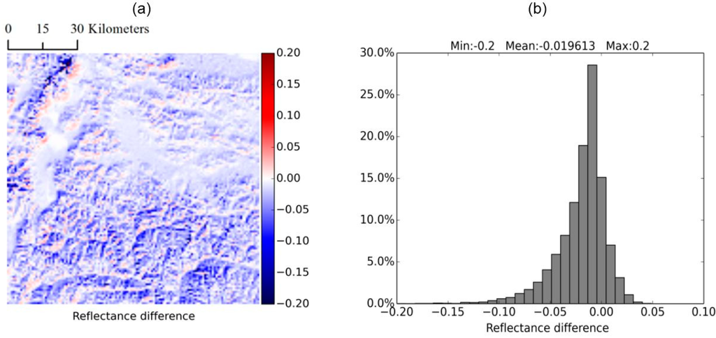
Figure 13. (a) Maps of the differences between reflectance values estimated from Landsat-7 band 8 with sub-pixel topographic reflectance as compared to the uncorrected reflectance value, (b) graph summarizing the distribution of those differences.

6. Conclusions

For several decades, the necessity to correct satellite data for atmospheric and topographic effects before being able to perform further data processing, especially when working with times series, is known and a lot of studies have been carried out on that issue. Recently, thanks to the increasing resolution of available global DEM, it is possible to explore new ways to improve the accuracy of surface reflectance data measured from space. One way to benefit from those higher spatial resolution data is to integrate the effects induced by topography at sub-pixel level on low spatial resolution satellite imagery, such as the data measured by geostationary satellites. The study presented in this paper, proposes an operational method to correct the retrieved surface reflectance measured from space for this sub-pixel topographic effects. Inspired from an existing pixel level topographic correction, this sub-pixel level topographic correction method shows better results in retrieving the surface reflectance from satellite data compared to pixel level topographic correction, especially in rough area as the one selected on the Tibetan Plateau. Those results, in line with the findings of Wen [19], could be very beneficial for the retrieval of reflectance form geostationary sensors such as MSG (Meteosat Second Generation), FY-2 (Feng-Yun) or GOES (Geostationary Operational Environmental Satellites), prior to be used for further products extraction. The larger differences observed between the two levels of correction are linked to the estimation of direct solar irradiance received by the surface, which is mainly controlled by the SBF. The estimation of the latter at sub-pixel level is crucial because it allows accounting for partial shadowing at pixel level. Indeed, as it is a binary parameter, it does not consider the possibility of partial shadowing of the pixel, while a significant fraction of the area covered by a kilometric pixel tagged as shadowed might actually see the sun. This can significantly affect the retrieved land surface reflectance values whereas 30 m resolution computations are much less affected by this discrepancy. In addition to the previous studies carried out on sub-pixel topographic heterogeneity, the integration of the adjacent terrain irradiance in the correction is a significant improvement as it represents an important contribution to the total irradiance when a pixel does not received direct sunlight. It is interesting to notice that the impact of the correction level depends on the period of the year and the time of the day, with a larger impact during the first and last hours of sunshine. The results clearly showed that the proposed methodology allowed for a better retrieval of surface reflectance, even if it tends to slightly overestimate the retrieved surface reflectance. This overestimation could probably be corrected by replacing the cosine law use in the first term of Equation (2) by a more efficient correction method. As the overestimation remains quite small so it could also be due to the surface Lambertian assumption when computing the irradiance reflected by the adjacent terrain. Even if the anisotropy properties of the land surface has been showed to be not the primary influencing factor, further investigations should be performed to integrate the anisotropy property of the surface in the sub-pixel topographic correction for the estimation of the terrain irradiance.

References

- Song, C.; Woodcock, C.E. Monitoring forest succession with multitemporal landsat images: Factors of uncertainty. IEEE Trans. Geosci. Remote Sens. 2003, 41, 2557–2567. [Google Scholar] [CrossRef]
- Turner, R.; Spencer, M. Atmospheric model for the correction of spacecraft data. In Proceedings of International Symposium on Remote Sensing of Environment, Ann Arbor, USA, 2–6 October 1972; pp. 895–934.
- Kaufman, Y.J. Atmospheric effect on spatial resolution of surface imagery. Appl. Opt. 1984, 23, 3400–3408. [Google Scholar] [CrossRef] [PubMed]
- Rahman, H.; Dedieu, G. SMAC: A simplified method for the atmospheric correction of satellite measurements in the solar spectrum. Int. J. Remote Sens. 1994, 15, 123–143. [Google Scholar] [CrossRef]
- Van Laake, P.E.; Sanchez-Azofeifa, G.A. Simplified atmospheric radiative transfer modelling for estimating incident PAR using MODIS atmosphere products. Remote Sens. Environ. 2004, 91, 98–113. [Google Scholar] [CrossRef]
- Jimenez-Munoz, J.C.; Sobrino, J.A.; Mattar, C.; Franch, B. Atmospheric correction of optical imagery from MODIS and reanalysis atmospheric products. Remote Sens. Environ. 2010, 114, 2195–2210. [Google Scholar] [CrossRef]
- Rochon, G.; Audirac, H.; Larrivee, A.; Beaubien, J.; Gignac, P. Radiometric Correction for Topographic Effects on Landsat Images of Forests. Available online: http://www.scopus.com/record/display.url?eid = 2-s2.0-0018624386&origin = inward&txGid = 3FA131ADAD37D0F58FD34FCFC8A0DC98.f594dyPDCy4K3aQHRor6A%3a1 (accessed on 1 September 2014).
- Kawata, Y.; Ueno, S.; Kusaka, T. Radiometric correction for atmospheric and topographic effects on Landsat MSS images. Int. J. Remote Sens. 1988, 9, 729–748. [Google Scholar] [CrossRef]
- Proy, C.; Tanre, D.; Deschamps, P.Y. Evaluation of topographic effects in remotely sensed data. Remote Sens. Environ. 1989, 30, 21–32. [Google Scholar] [CrossRef]
- Meyer, P.; Itten, K.I.; Kellenberger, T.; Sandmeier, S.; Sandmeier, R. Radiometric corrections of topographically induced effects on Landsat TM data in an alpine environment. ISPRS J. Photogramm. Remote Sens. 1993, 48, 17–28. [Google Scholar] [CrossRef]
- A robust algorithm for correcting the topographic effect of satellite image over mountainous terrain. Available online: http://www.isprs.org/proceedings/xxxi/congress/part7/105_XXXI-part7.pdf (accessed on 1 September 2014).
- Richter, R. Correction of atmospheric and topographic effects for high-spatial-resolution satellite imagery. Int. J. Remote Sens. 1997, 18, 1099–1111. [Google Scholar]
- Wen, J.; Liu, Q.; Liu, Q.; Xiao, Q.; Li, X. Parametrized BRDF for atmospheric and topographic correction and albedo estimation in Jiangxi rugged terrain, China. Int. J. Remote Sens. 2009, 30, 2875–2896. [Google Scholar] [CrossRef]
- Riano, D.; Chuvieco, E. Assessment of different topographic corrections in Landsat-TM data for mapping vegetation types. IEEE Trans. Geosci. Remote Sens. 2003, 41, 1056–1061. [Google Scholar] [CrossRef]
- Richter, R.; Kellenberger, T.; Kaufmann, H. Comparison of topographic correction methods. Remote Sens. 2009, 1, 184–196. [Google Scholar] [CrossRef]
- Szantoi, Z.; Simonetti, D. Fast and robust topographic correction method for medium resolution satellite imagery using a stratified approach. IEEE J. Sel. Top. Appl. Earth Obs. Remote Sens. 2013, 6, 1921–1933. [Google Scholar] [CrossRef]
- Kustas, W. Evaluating the effects of subpixel heterogeneity on pixel average fluxes. Remote Sens. Environ. 2000, 74, 327–342. [Google Scholar] [CrossRef]
- Liu, W.; Hu, B.; Wang, S. Improving land surface pixel level albedo characterization using sub-pixel information retrieved from remote sensing. In Proceedings of the IEEE Geoscience and Remote Sensing Symposium, Boston, MA, USA, 7–11 July 2008; pp. 801–804.
- Wen, J.; Liu, Q.; Liu, Q.; Xiao, Q.; Li, X. Scale effect and scale correction of land-surface albedo in rugged terrain. Int. J. Remote Sens. 2009, 30, 5397–5420. [Google Scholar] [CrossRef]
- Roman, M.O.; Gatebe, C.K.; Schaaf, C.B.; Poudyal, R.; Wang, Z.; King, M.D. Variability in surface BRDF at different spatial scales (30 m–500 m) over a mixed agricultural landscape as retrieved from airborne and satellite spectral measurements. Remote Sens. Environ. 2011, 115, 2184–2203. [Google Scholar] [CrossRef]
- Li, P.; Shi, C.; Li, Z.; Muller, J.-P.; Drummond, J.; Li, X.; Li, T.; Li, Y.; Liu, J. Evaluation of ASTER GDEM using GPS benchmarks and SRTM in China. Int. J. Remote Sens. 2013, 34, 1744–1771. [Google Scholar] [CrossRef]
- Measures of Shape: Skewness and Kurtosis. Available online: http://oakroadsystems.com/math/3shape.htm (accessed on 27 December 2012).
- Sandmeier, S.; Itten, K.I. A physically-based model to correct atmospheric and illumination effects in optical satellite data of rugged terrain. IEEE Trans. Geosci. Remote Sens. 1997, 35, 708–717. [Google Scholar] [CrossRef]
- Richter, R. Correction of satellite imagery over mountainous terrain. Appl. Opt. 1998, 37, 4004–4015. [Google Scholar] [CrossRef] [PubMed]
- Shepherd, J.D.; Dymond, J.R. Correcting satellite imagery for the variance of reflectance and illumination with topography. Int. J. Remote Sens. 2003, 24, 3503–3514. [Google Scholar] [CrossRef]
- Baraldi, A.; Gironda, M.; Simonetti, D. Operational two-stage stratified topographic correction of spaceborne multispectral imagery employing an automatic spectral-rule-based decision-tree preliminary classifier. IEEE Trans. Geosci. Remote Sens. 2010, 48, 112–146. [Google Scholar] [CrossRef]
- Parametric Bidirectional Reflectance Factor Models: Evaluation, Improvements and Applications. Available online: file:///C:/Users/MDPI/AppData/Local/Temp/CLNA16426ENC_001.pdf (accessed on 1 September 2014).
- Rahman, H.; Verstraete, M.M.; Pinty, B. Coupled surface-atmosphere reflectance (CSAR) model 1. Model description and inversion on synthetic data. J. Geophys. Res. 1993, 98, 20779–20789. [Google Scholar] [CrossRef]
- Kastendeuch, P.P. A method to estimate sky view factors from digital elevation models. Int. J. Climatol. 2013, 33, 1574–1578. [Google Scholar] [CrossRef]
- Oke, T.R. Boundary Layer Climates, 2nd ed.; Routledge: London, UK, 1987. [Google Scholar]
- Dozier, J.; Frew, J. Rapid calculation of terrain parameters for radiation modeling from digital elevation data. IEEE Trans. Geosci. Remote Sens. 1990, 28, 963–969. [Google Scholar] [CrossRef]
- Zaksek, K.; Ostir, K.; Kokalj, Z. Sky-view factor as a relief visualization technique. Remote Sens. 2011, 3, 398–415. [Google Scholar] [CrossRef]
- Vanonckelen, S.; Lhermitte, S.; Rompaey, A.V. The effect of atmospheric and topographic correction methods on land cover classification accuracy. Int. J.Appl. Earth. Obs. 2013, 24, 9–21. [Google Scholar] [CrossRef]
© 2014 by the authors; licensee MDPI, Basel, Switzerland. This article is an open access article distributed under the terms and conditions of the Creative Commons Attribution license (http://creativecommons.org/licenses/by/4.0/).