Article

Satellite-Based Sunshine Duration for Europe

1
Institute for Atmospheric and Environmental Sciences, Goethe-University Frankfurt, Altenhöferallee 1, D-60438 Frankfurt, Germany
2
Met Office Hadley Centre, FitzRoy Road, Exeter, Devon EX1 3PB, UK
3
Deutscher Wetterdienst, Frankfurter Str. 135, Offenbach D-60387, Germany
*
Author to whom correspondence should be addressed.
Remote Sens. 2013, 5(6), 2943-2972; https://doi.org/10.3390/rs5062943
Submission received: 24 April 2013 / Revised: 30 May 2013 / Accepted: 3 June 2013 / Published: 7 June 2013

Abstract

:
In this study, two different methods were applied to derive daily and monthly sunshine duration based on high-resolution satellite products provided by the European Organisation for the Exploitation of Meteorological Satellites (EUMETSAT) Satellite Application Facility on Climate Monitoring using data from Meteosat Second Generation (MSG) SEVIRI (Spinning Enhanced Visible and Infrared Imager). The satellite products were either hourly cloud type or hourly surface incoming direct radiation. The satellite sunshine duration estimates were not found to be significantly different using the native 15-minute temporal resolution of SEVIRI. The satellite-based sunshine duration products give additional spatial information over the European continent compared with equivalent in situ-based products. An evaluation of the satellite sunshine duration by product intercomparison and against station measurements was carried out to determine their accuracy. The satellite data were found to be within ±1 h/day compared to high-quality Baseline Surface Radiation Network or surface synoptic observations (SYNOP) station measurements. The satellite-based products differ more over the oceans than over land, mainly because of the treatment of fractional clouds in the cloud type-based sunshine duration product. This paper presents the methods used to derive the satellite sunshine duration products and the performance of the different retrievals. The main benefits and disadvantages compared to station-based products are also discussed.

1. Introduction

Sunshine duration (SD), together with surface temperature and precipitation, is one of the most important and widely used parameters in climate monitoring and a key variable for various sectors, including tourism, public health, agriculture [1], vegetation modeling [2], and solar energy. Although not specifically defined as an Essential Climate Variable by the Global Climate Observing System, SD is strongly related to the Essential Climate Variables cloud properties and surface radiation budget. SD is also used as an input parameter for hydrological modeling [3] and is a good predictor for the estimation of global radiation (e.g., [48]) where it can be also used for quality control of measured global radiation data [9].
Historical records of SD date back more than a century. In the mid-19th century, the Campbell–Stokes sunshine recorder was invented—much earlier than the first pyranometer. Even today, Campbell–Stokes recorders are still used by many national weather services. The continuation of these long time series is of importance e.g., for climatological studies. As sunshine duration data are a good proxy for global and direct solar radiation (e.g., [68]), the observed decadal variation of sunlight at the Earth’s surface is, for example, an object of research in the context of global dimming and brightening [10,11]. Trends and variability of SD have recently been described for several regions of the world, e.g., South America [12], India [13] and Western Europe [14].
Another very important reason for the use of SD is that it is easy to understand. SD is very established in media, and the public is used to this parameter. The hours of sunshine per day are much easier to handle for most non-scientific people than a value in W/m2. Thus, SD is especially important for national weather services and federal authorities to communicate with the public or decision makers.
SD is a standard parameter at meteorological stations and its measurement is specified by the World Meteorological Organization (WMO) [15]. The possibility of mapping SD by using station observations is limited, given that the density of stations is very heterogeneous and many regions suffer from a coarse station network. Also, station observations are point measurements with a limited representativeness for larger regions. To extend the spatial information of station data, some national meteorological and hydrological services produce gridded maps of interpolated SD station measurements, e.g., the UK Met Office [16] and the German Meteorological Service DWD [17]. For the WMO region VI (Europe and the Middle East), operational station-based SD maps are produced by the WMO Regional Climate Centre on Climate Monitoring [18], and the Climatic Research Unit provides a global SD climatology over land areas [19].
Station-based gridded products incorporate spatial interpolation techniques. For example, Dolinar [20] used Kriging for the generation of SD maps for Slovenia. Hogewind and Bissolli [21] described several interpolation methods for the construction of operational climate maps for Europe and the Middle East. Station-based products are subjected to several problems. For example, the uncertainty of the interpolation strongly increases in areas with a low station density and the interpolation has to account for the influence of topographic features. Moreover, SD itself is highly variable as it depends on cloud fraction, which is highly heterogeneous and exhibits strong temporal dynamics.
Due to the ability of space-borne instruments to detect clouds and the correlation of SD with cloud cover [22], satellite data can be used for the estimation of SD and add valuable information to station-based products. For instance, Kandirmaz [23] used a statistical relationship between daily mean cloud cover index and measured SD to derive daily global SD from geostationary satellite data. Kandirmaz [23] tested this method on data from the Meteosat First Generation. Journée et al. [24] derived SD maps for Belgium and Luxembourg from Meteosat First Generation global and direct solar radiation by help of the Ångström–Prescott equation [25]. More recently, Good [26] used 15-minute time series of cloud type (CTY) data from Meteosat Second Generation (MSG) to compute daily SD for the United Kingdom. The study by Good [26] is the first one that used the high potential of the MSG SEVIRI (Spinning Enhanced Visible and Infrared Imager) instrument to derive SD. This imager offers a larger selection of channels for more complex products with a higher spatial resolution compared with Meteosat First Generation. However, Good [26] applied this method to the relatively small region of United Kingdom, which allowed no conclusions for other European regions with different climatic influences, high mountains, or limited ground-based observations.
The aims of this study are:
(i)
to extend the Good [26] CTY method to the wider region of Europe in order to enable the provision of sunshine duration products for the whole region and to support countries with limited ground-based observations or lacking adequate production systems,
(ii)
to propose a new method where SD is computed using solar incoming direct radiation (SID) and the WMO threshold for sunshine of 120 W/m2, and
(iii)
to compare the results against station-based SD data, and each other.
The 120 W/m2 threshold for SID is based on Campbell–Stokes recorders, which were used for SD measurements since the mid-19th century. Investigations showed that the threshold irradiance for burning the cards was on average 120 W/m2[15]. In 1981, this threshold was recommended by the Commission for Instruments and Methods of Observation [15] to distinguish bright sunshine.
Both the CTY and SID datasets used here are provided by the European Organisation for the Exploitation of Meteorological Satellites (EUMETSAT) Climate Monitoring Satellite Application Facility (CM SAF). Daily and monthly sums of the satellite-based products will be compared with station data as well as gridded station data. Our analysis focuses on the year 2008 and examines the feasibility and validity of both daily and monthly satellite SD totals. The MSG SEVIRI instrument offers a temporal resolution of up to 15 minutes in operational mode. Thus, it is also of interest to establish whether there is a significant change in the satellite SD estimates when the temporal resolution changes from 15 min (as used by Good [26]) to 1 h, which would be substantially less computationally demanding.
Sections 2 and 3 give a description of the applied data and retrieval methods. Examples of both the CTY- and SID-based products are shown in Section 4. Additionally, in Section 4 the satellite SD products are compared with point and gridded station observations, to estimate the uncertainties, advantages, and disadvantages of satellite-based SD. Finally, the difficulties in retrieving SD from satellites are discussed.

2. Data

The satellite SD estimates were derived from either CTY or SID products provided by the CM SAF. These CTY and the SID retrievals are based on data from the SEVIRI instrument onboard the geostationary Meteosat Second Generation (MSG) satellites, Meteosat-8 and Meteosat-9. The native resolution for MSG based products is 15 min in the temporal, and about 3 km (nadir) in the spatial dimension. Both products apply the same SEVIRI-based cloud mask to distinguish between cloud-free, cloud-contaminated, and cloud-filled pixels [27].

2.1. SEVIRI Cloud-Type Product (CTY)

The algorithms for the SEVIRI CTY product were developed by the EUMETSAT Satellite Applications Facility on Nowcasting in order to support nowcasting and very short-range forecasting. The product used in this study was obtained through the CM SAF. Using a multi-spectral threshold method, information for all major cloud classes is retrieved. This method is based on the fact that cloud properties, such as height, amount, texture, or cloud phase are dependent on their brightness temperature and reflectance. Every pixel, which is marked as cloudy or cloud-filled by the cloud mask, is classified by a threshold procedure, which is applied to different channels and channel combinations for spectral and textural features [27]. The thresholds chosen depend on several factors, such as illumination conditions, viewing geometry, geographical location, numerical weather prediction data, water vapor content, and the coarse vertical structure of the atmosphere. Also, the retrieval uses different channels, channel combinations, and thresholds for daytime, twilight, nighttime, and land or sea. Overall the retrieval uses seven spectral channels, of which four are mandatory and three optional. Due to missing observations and different cloud definitions of other satellite products, there is no robust evaluation of this product. However, there are some known problems of the CTY-product: thin cirrus can be misclassified as fractional clouds, very low clouds can be classified as medium clouds in cases of strong thermal inversions, or low clouds surmounted by thin cirrus may be misclassified as medium clouds [27].

2.2. SEVIRI Surface Incoming Direct Radiation (SID)

The SEVIRI SID product used in this study is also provided by the CM SAF [28]. This product is part of the retrieval of the surface incoming short-wave radiation. For clear sky cases the surface incoming short-wave radiation product is completely based on a radiation transfer model. For pixels set by the cloud mask to partly cloudy or filled with semitransparent clouds, a semi-empirical approach [29,30] is applied. For fully cloudy pixels the fraction of SID that is able to penetrate a cloud is determined depending on the cloud thickness (expressed by the clear sky index as a measure for the transmissivity of the atmosphere). Besides the cloud mask, the quality of the SID product depends strongly on the input parameters for the radiation transfer model, such as aerosols, water vapor, ozone, and the clear sky index. The accuracy of SID monthly means is estimated by CM SAF to be better than 15 W/m2[31].

2.3. Reference Station Data

For evaluation purposes, data from the surface synoptic observations (SYNOP) and CLIMAT observation station network were used in this study. SYNOP data are available from a large number of synoptic stations all over the world. These data are distributed several times a day, and are mainly intended for usage in weather forecasting [21]. The data consist of daily or sub-daily observations. In contrast, the main application for CLIMAT data is climate analyses and these data are therefore monthly totals. The CLIMAT data undergo routine quality control at DWD. CLIMAT and SYNOP sunshine duration data are only available for land-based stations.
For our analysis, some basic quality checks were also applied to the daily SYNOP data. Stations were omitted from the analysis if they reported SD totals exceeding day length, or hourly sums, which did not match the reported daily totals. The Italian stations only report hourly values, so daily sums had to be calculated separately and additional quality checks were performed. Stations were removed from the analysis if they reported apparently erroneous data, such as fixed zeros or permanently high values throughout the year.
SYNOP and CLIMAT station data are available for a relatively high number of stations, but despite quality checks, there is no guarantee that these data are bias free. To have some high quality station data for comparisons, we also used data of the Baseline Surface Radiation Network (BSRN). BSRN is a project aiming at the detection of changes in the earth’s surface radiation [32]. This network contains quality controlled observation stations with a high accuracy [33]. There are only a few stations in Europe. For our comparisons, four BSRN stations were used. In addition, data from the DWD station in Lindenberg (Germany) were used for evaluation. The Lindenberg station also offers high quality radiation data. All BSRN stations use Kipp and Zonen instruments to measure SD.
In this study, the gridded satellite SD products are evaluated at daily and monthly timescales using the SYNOP data. The daily SYNOP station data are therefore used to generate monthly totals at each station. Up to three days of missing data are permitted per month at each station. The monthly totals are scaled up to account for missing data using the daily average SD for that month. Where more than three days of missing data occur, the station is excluded from the analysis for that month.
In the framework of the WMO Regional Climate Centre on Climate Monitoring for the WMO Region VI (Europe and the Middle East), DWD provides a spatial gridded product for SD (in the following referred to as SD-RCC product) (see Product Description Sheet at [18]). This product is based on monthly CLIMAT data for the WMO region VI and therefore represents monthly SD totals. For Europe, there are about 380 CLIMAT stations included in this dataset. However, the station density is very inhomogeneous. For example, there are only few stations in Scandinavia and Eastern Europe, while there is a high density in Germany. This is particularly problematic for the interpolation of a heterogeneous parameter, such as SD. The interpolation technique applied uses a linear regression of sunshine duration with latitude, longitude and altitude and then applies Radial Basis functions for the spatial interpolation of CLIMAT station data to a grid with a horizontal resolution of 0.1° [21]. Despite this sophisticated interpolation technique, the interpolation of station data can be problematic in data sparse regions, in regions with strong topography, or due to insufficient representativeness. Thus, it is of high interest to compare these data with satellite-based products.

3. Methods: Generation of Satellite-Based SD Estimates

For derivation of satellite-based SD two different methods were applied to generate daily SD estimates. The first method is based on CTY observations, following Good [26], and is described in Section 3.1. The second method is similar, but uses sub-daily SID data (Section 3.2). Although the native temporal resolution of SEVIRI is 15 min, the satellite SD product generation was trialed using both 15-minute and hourly data. Using hourly data is preferable as the data volumes are significantly smaller and processing less computationally expensive. The results of this trial are presented in Section 3.3.
Monthly satellite SD totals are also calculated in this study and are compared with the SD-RCC product described in Section 2. The monthly satellite SD data are generated from the daily sums on a pixel-by-pixel basis. Due to more than three missing days, the monthly totals of May and December 2008 are unavailable for this study. If there are one to three missing days, the monthly totals are scaled up to account for that by using the daily average SD for that month.

3.1. SD Derivation Using CTY Data (SD-CTY Product)

The method proposed by Good [26] is based on the Satellite Applications Facility on Nowcasting CTY product. In essence, the method takes a sub-daily time series of CTY observations during daylight hours to estimate the SD for each day. For each observation slot, each pixel is assigned either bright sunshine or no sunshine. The daily SD total (SDTotal) is then calculated according to:
SD Total = N bright _ sunshine N Total H
where N is the number of SEVIRI observation slots and H is the number of hours of daylight.
The CTY product has 19 different cloud classes. If there is no cloud, bright sunshine is assumed. For opaque clouds there is no sunshine. In case of fractional clouds a factor of 0.5 is assumed following Good [26]. For semi-transparent clouds, bright sunshine is assumed if the solar elevation angle exceeds a specific threshold.
The biggest challenge in the context of deriving SD by using CTY products is the treatment of fractional and semi-transparent clouds. Good [26] used the online available Fu–Liou radiation code to derive the solar elevation angle thresholds for assumed cloud properties of three different cirrus clouds. To cover a wider variety of cirrus clouds, in this study, the solar elevation angle thresholds for the three classes of semi-transparent clouds were derived using a linear regression between the solar elevation angle and the normalized SID, using hourly data for each month of the year 2008. The normalization is done to be consistent with in situ observations, which are done for the perpendicular component of SID. Good [26] did not use this normalization, which could lead to uncertainties. The normalized SID (SIDNorm) is the ratio of SID and the cosine of the solar zenith angle (SZA):
SID Norm = SID cos ( SZA )
In deriving the thresholds for each cirrus cloud class of the CTY product (15: very thin, 16: thin, 17: thick), data with solar elevation angle <2.5° were not used, following Good [26], who reports ground-based instruments are unlikely to record bright sunshine for solar elevation angles less than this value. Also we did not use data with SIDNorm < 50 W/m2, so as to capture the thresholds better by a linear regression. The solar elevation threshold is the angle below which SIDNorm is less than the WMO criterion of 120 W/m2 according to these regressions.
For each day, all pixels that fulfilled these requirements were collected and a linear regression between SIDNorm and the corresponding solar elevation angle applied. The resulting thresholds were averaged over each month (Table 1). The thresholds demonstrate an annual cycle, with a maximum in summer. The explained variances (R2) for the regressions between SIDNorm and the corresponding solar elevation angle are high (typically 0.8–0.9) and quite consistent throughout the year for cloud classes 15 and 16 (Table 1, in brackets). The R2 for class 17 is lower (0.5–0.6), but with higher values in winter (∼0.8).

3.2. SD Derivation Using SID Data (SD-SID Product)

The SID method is based on a sub-daily time series of the CM SAF SID product. According to the WMO, bright sunshine occurs when the solar direct radiation exceeds 120 W/m2[15]. Modern Kipp and Zonen sunshine detectors measure in the direction of the sun, while the satellite-based SID product assumes a horizontal plane [28]. To account for this directional discrepancy, the SID product was normalized by the solar zenith angle to ensure consistency with in situ observations.
The solar elevation angle limit of 2.5° was adopted for consistency with the CTY method (Section 3.1). Owing to problems with the CM SAF SID retrieval at low solar elevation angles (SEA), there is a sharp transition in the twilight zone of this product, which causes some artifacts in the resulting SD product. Varying the 2.5° solar elevation angle threshold was found to have only minor effects on these artifacts. These artificial patterns are visible mainly in daily totals, but are also visible in some monthly totals, and can influence the quality of the SD products. In the twilight zone of the SID product there are values cut, which were larger than 0. Thus, it is possible that the resulting SDSID product has values that are too low in these areas.
The CM SAF validation report specifies for the SID product an accuracy within 15 W/m2. To investigate the impact of this uncertainty the SD-SID product was generated for SIDNorm thresholds of 105 W/m2 and 135 W/m2. Table 2 shows the impact of varying this threshold on monthly SD totals from 2008, and demonstrates that the effect of this uncertainty on the resulting SD-SID product is negligible.

3.3. Comparison of Hourly and 15 Min Satellite SD Products

Clouds, which show strong temporal dynamics, are the main influencing factor for calculation of SD using both the CTY and SID methods. Good [
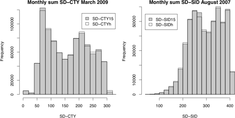
26] used 15-minute data to generate daily SD-CTY estimates from SEVIRI. In this section, example satellite SD products were generated using both 15-minute and hourly input data to assess any impact of using the lower temporal resolution input data. Results for the months of March 2009 for SD-CTY, and August 2007 for SD-SID are presented. The CM SAF generally stores CTY and SID products only on an hourly basis, and these two months were chosen due to the availability of 15-minute CTY and SID data.
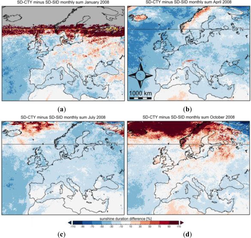
Table 3 shows some simple statistics comparing the monthly satellite SD totals generated using the 15-minute and hourly input data. In each case the mean difference is around 30 min, which equates to less than 0.4% of the monthly mean SD total. The spatial pattern of these differences is non-systematic (Figure 1), with no clear tendency for higher or lower SD values for one of the two time resolutions. Figure 2 shows the distributions of monthly SD totals for each product, using input data with both temporal resolutions. The results show that changing the temporal resolution from 15 min to 1 h has only a very tiny effect on the overall monthly SD distributions.
In light of these findings, the satellite SD products used in the remainder of this article were generated using input data at hourly resolution, as the additional computational expense required to process the 15-minute data cannot be justified.

4. Results

A goal of this study is the application of simple methods to derive a satellite-based SD dataset by using existing products of the EUMETSAT SAFs. The SD-SID method is a direct method, which checks for exceedances of one clearly defined threshold. The SD-CTY method is more involved and needs some approximation for dealing with cirrus and fractional clouds. Neither method involves direct measurement of sunshine duration and in each case, the input satellite data have their own uncertainties. Therefore, an intercomparison of the satellite SD products allows the estimation of uncertainties especially in regions without station measurements.

4.1. Satellite SD Products Comparison

Figure 3 shows some examples of monthly totals for both types of satellite products for January, April, July and October 2008, while Figure 4 shows the corresponding differences between the two products (SD-CTY minus SD-SID). Both the SD-CTY and SD-SID products show similar spatial patterns, but the SD-SID values are typically higher than SD-CTY for all four months, particularly for ocean pixels. All the maps in Figure 3 show a north-to-south increase in SD, with very high SD values occurring in northern Africa. In contrast, the SD is lower at these latitudes in the Atlantic Ocean. Higher values of SD are also observed in both products over the Mediterranean Sea compared with the surrounding European landmasses. For example, in April 2008, SD values of 250 h are observed over the Mediterranean Sea, which is the highest value in Europe for this month. Sharp land–sea SD contrasts are also observed in many places for all months, but are particularly evident in the April and July examples around the Mediterranean basin and northern European coastlines.
Depending on the season, the MSG viewing geometry allows a reliable SID/CTY retrieval up to about 60° latitude, which will then propagate through to the SD-SID and SD-CTY estimates. The January panels in Figures 3 and 4 illustrate for SD-SID that this limit is about 57°N, beyond which there is a decrease in the SD-SID product reliability, which must be taken into account in any analysis. Otherwise, the strongest differences between SD-CTY and SD-SID occur in the Mediterranean region, where the winter is the season with the highest cloud fraction.
For the July 2008 totals, there is a strong gradient visible at about 65°N, and values north of this latitude must be discarded. Noticeable is the Baltic Sea where the SD is higher than in the surrounding area. The relatively low cloud fraction in summer in the Mediterranean leads to a high SD in this region. Another remarkable feature is the relatively low SD along the eastern coast of the Black Sea, which corresponds to the high precipitation amounts in this region. The values of SD-SID exceed SD-CTY in most parts of the domain.
The best agreement between SD-SID and SD-CTY is found over land regions such as Central Europe, the Iberian Peninsula or Northern Africa with differences of about −20% to −25%. Over the Atlantic Ocean, especially south of the Azores, the differences in some cases are more than −50% (which is more than −100% in reference to SD-CTY) (see Figure 4). Higher values of SD-CTY compared to SD-SID are mainly restricted to some months in the Alps or Northern Africa. Considering Figures 3 and 4 it has to be kept in mind that values north of 55°N to 60°N are not reliable.

4.2. Comparison with BSRN Station Data

For the comparisons in this section, four BSRN stations and the DWD station Lindenberg were used. A mean of nine satellite pixels centered on each station was used for the evaluation.
Figure 5 shows the daily evaluation results for Cabauw for 2008. Table 4 summarizes the correlations, the mean satellite SD product minus station SD differences, and the ratio of the satellite product to station standard deviations for all five stations (i.e., satellite standard deviation/station standard deviation). The correlations in the Taylor diagram (Figure 5(b)) and in Table 4 are high with values of more than 0.9. However, it should be noted that these correlations might be influenced by the annual cycle of SD. The impact of the annual cycle on the correlations in Table 4 was estimated by considering the ratio of the explained variance of a sine-shaped annual cycle divided by the explained variance of the satellite product (R2(station vs. sine curve)/R2(station vs. satellite product)). If this ratio is zero, there is no influence of the annual cycle, and if this ratio is larger than one, the projection of the annual cycle is larger than that of the satellite product. The scatter plot (Figure 5(a)) and the mean differences in Table 4 show that in many cases SD-CTY underestimates SD and SD-SID overestimates SD. The root mean square difference was in all cases between 1 and 2 h. In light of the annual mean daily SD for Central Europe, which is about 5 h, this is an uncertainty of up to 40%.

4.3. Comparison with SD-RCC Data

Figures 6, 7 and 8 show spatial subsets of the SD-SID and SD-CTY monthly totals for July 2008 compared with the corresponding subsets from the station-based SD-RCC product. The region shown in Figure 6 comprises an area of 5° latitude times 15.6° longitude. This quite large area is covered in SD-RCC by only eight heterogeneously distributed observation stations (Figure 6, black dots). The satellite-based product is much more detailed, and even shows the influence of the Dnieper River and the Carpathians on SD. Further examples for the south of France and the Balkans (Figures 7 and 8) also show that the satellite product illustrate the heterogeneous patterns of SD in much more detail than the corresponding SD-RCC product. In the SD-RCC product, small-scale landscape features between the stations are only captured by the use of altitude information. Thus, the direct or indirect influence of rivers, lakes, different land surface types, mountain shadowing, and of course clouds, is only included in the satellite-based products.

4.4. Comparison with SYNOP Station Data

This section describes the evaluation of both the SD-CTY and SD-SID daily and monthly sum satellite products using the SYNOP station data described in Section 2.3. The evaluation is performed by comparing single-pixel satellite SD with collocated station observations, where the SEVIRI pixel selected nominally contains the station location. Evaluation is performed for all available days/months in 2008.

4.4.1. Daily Evaluation Results

Figure 9 shows time series of the mean and standard deviation of the satellite-based SD minus station SD, together with the correlation between the satellite and station data for each day. The results indicate that the agreement between the SD-SID product and station data is more stable than for the SD-CTY product. This is evidenced by lower standard deviations (e.g., 80% days have standard deviation ≤ 2.0 h for SD-SID, compared with 45% for SD-CTY) and higher Pearson correlation coefficient (e.g., 99% of days have correlation >0.8, compared with 71% for SD-CTY). However, the SD-SID product is more strongly biased than SD-CTY, with a mean daily bias (satellite minus station) of +0.8 h compared with −0.1 h for SD-CTY. These relative biases (i.e., SD-SID overestimating and SD-CTY underestimating SD with respect to station data) are consistent with the BSRN evaluation results presented in Section 4.2. Both products exhibit a seasonal cycle in their agreement with the station data, where the agreement is best in winter months and worst in summer months. For the SD-CTY product, the daily bias becomes more negative in the summer, which is consistent with the results of Good [26]. Interestingly, the seasonal cycle in the SD-SID bias has the opposite sense, becoming more positive in the summer months.
Figure 10 shows maps of the mean and standard deviation of the daily satellite minus station SD for each station in January 2008 for the SD-SID and SD-CTY products, respectively. Also shown are the differences between the two sets of validation results (i.e., results for SD-SID minus results for SD-CTY). Figure 11 shows the equivalent plots for July 2008. The figures suggest there are some individual stations where the satellite–station agreement is particularly poor, for example, around the Alps. There are also some spatial patterns evident: for example, low standard deviations in Turkey and the Iberian Peninsula in July, while those in the northeastern part of Europe are particularly high. Mean station biases in Eastern Europe are also notably lower in July than elsewhere.
To estimate if these patterns may be attributed to factors such as elevation or satellite viewing angle, the variation in station validation statistics for both satellite SD products for each month of the analysis as a function of elevation and SEVIRI zenith angle is investigated (not shown). The elevation data used correspond to the SEVIRI pixel elevation static data. The zenith angle is calculated from the known satellite viewing geometry, curvature of the earth and earth location of the station. The number of satellite–station matches varies between 775 and 1,126, depending on the month and datasets used; January and December have the lowest number of matches.
Overall, there seems to be only a small relationship between bias and elevation, particularly for the SD-CTY product, with many months showing relationships that are insignificant at the 5% level. However, the correlation between standard deviation and elevation is much stronger, peaking during the winter months where higher standard deviations occur at higher elevations. These results imply that it is mostly the variance of the satellite SD products that is affected by surface elevation, with the effects being more apparent in the SD-SID product.
For both SD-CTY and SD-SID, there is a clear relationship between satellite SD and zenith angle. For the SD-CTY product, the relationship is strongest in the summer months with correlations reaching 0.58 (August). The mean daily bias becomes more negative with increasing zenith angle, while the standard deviation increases with zenith angle between March and September, but decreases for other months. For the SD-SID product, the bias also becomes more negative with increasing zenith angle although there is no clear seasonal cycle in this relationship. However, the standard deviations show a seasonal cycle, with peak correlations (up to 0.33) and slopes occurring during June, July and August. As for the SD-CTY product, standard deviations increase with zenith angle between March and August, but decrease for other months. Overall, the results indicate a more negative bias with increasing zenith angle in the satellite SD, with increased variance during the summer months. A similar analysis looking at variation of satellite–station agreement as a function of land cover was also performed (not shown), but no relationship was evident.

4.4.2. Monthly Evaluation Results

The results presented in Section 4.4.1 demonstrate that the satellite SD products provide estimates that agree well with station observations on daily timescales. However, as some users will require monthly SD estimates it is also useful to determine how any biases propagate through to this longer timescale. In addition to comparing the satellite monthly totals with collocated station observations, an equivalent evaluation of the monthly station-based SD-RCC product was also performed for comparison. As the SD-RCC product is generated by gridding observations from CLIMAT stations, the SD-RCC and satellite products were evaluated using only SYNOP stations that do not report monthly CLIMAT messages.
Figure 12 shows the monthly evaluation results for each product. The results indicate that the SD-RCC product performs better than both satellite products in terms of bias, standard deviation and correlation. The SD-RCC products demonstrate only a small mean bias (<10 h) compared with the station data, whereas the SD-CTY and SD-SID products exhibits biases of −20 to 10 h and +10 to +40 h, respectively. As for the daily evaluation, the SD-SID product performs better than the SD-CTY product in terms of standard deviation and correlation, but has a bias of larger magnitude. All products show similar seasonal cycles for standard deviation and correlation with larger variance and lower correlations generally observed during summer months.
To assess the impact of excluding CLIMAT stations in the monthly evaluation, Figure 13 shows the SD-SID results from Figure 9 using both all available stations (i.e., including CLIMAT), and non-CLIMAT stations only. The results indicate that the effect of excluding the CLIMAT stations from the analysis is very small, causing only a small increase (decrease) in the standard deviation (correlation), with only a negligible effect on the bias.
Table 5 shows the mean bias of the SD-RCC product monthly totals as a function of the grid-box elevation used in the SD-RCC interpolation scheme (see Section 2.3). There is a small but significant relationship between these two parameters, which peaks during the summer months and is at a minimum during winter. For example, the slopes indicate that biases in the SD-RCC monthly totals of up to around 16 h in winter and 39 h in summer may occur at heights of 3,000 m as a result of elevation effects. This is comparable with the magnitude of the daily biases for the satellite products, although in this case, the relationships are not always significant at the 5% level.
Table 5 also shows the relationship between the bias in the SD-RCC monthly totals, and the distance between each SD-RCC grid box validated with SYNOPs and the nearest CLIMAT station used in that monthly SD-RCC total (i.e., grid box center to station distance). In previous sections (e.g., Sections 2.3 and 4.3) it was noted that the SD-RCC product is produced by interpolating CLIMAT station data, but that the CLIMAT network is often sparse. The objective of this second set of statistics is therefore to determine whether there is any degradation in quality of the SD-RCC product in areas where the CLIMAT network density is low. The results in Table 5 suggest this is probably not the case, with half of the slope/correlation pairs being insignificant at the 5% level. Where the results are significant, the bias vs. distance slope is low (less than 5.6 h monthly total per degree) with no consistent pattern in the trends or even the signs of the trends. This suggests that the quality of the SD-RCC product is only slightly affected by the station network density.
However, there is a caveat in making this statement. Not every SD-RCC grid box has been validated with independent non-CLIMAT SYNOP stations. Furthermore, grid boxes that have been validated tend to lie close to the CLIMAT stations used in the SD-RCC product interpolation. In fact, when we consider the entire SD-RCC product, the grid-cell-to-nearest CLIMAT station distance ranges between 0 and 24.5 degrees, with 59% of boxes lying within 2 degrees and 79% within 5 degrees. For the independent, non-CLIMAT SYNOP station evaluation performed here, all the SYNOP stations used correspond to SD-RCC grid boxes where the nearest CLIMAT station is within 5 degrees, with 95% within 2 degrees. In summary, we have not been able to properly assess the accuracy of the SD-RCC product where the grid-box-to-nearest CLIMAT station distance is between 2 and 5 degrees, which accounts for 20% of the SD-RCC product. Furthermore, no assessment of the SD-RCC product has been performed for grid-box-to-nearest CLIMAT station distances greater than 5 degrees, which corresponds to 21% of the SD-RCC product. Together, these situations account for more than 40% of the SD-RCC product that has been generated in the most challenging conditions where there are no CLIMAT stations within 2 degrees latitude/longitude.

5. Discussion

The main goals of this study were the application and evaluation of two different methods to derive SD from satellite-based products for the European region. The adaption of the Good [26] method showed a challenge, which is explained in the first part of this discussion (Seasonal cycle in SD-CTY). To estimate the uncertainty of SD-CTY and SD-SID, a product intercomparison was performed. This comparison showed significant differences especially over ocean areas, which are discussed in the second paragraph (Satellite-based products intercomparison). The best references to evaluate the satellite-based SD products are station observations. However, since these station data are very heterogeneously distributed, the evaluation is combined with problems, which are regarded in the third part of this discussion (Comparison with station data). Station-based gridded SD-RCC data are the only available alternative for our satellite-based SD products. However, these data suffer from deficiencies of the interpolation technique, which makes the comparison difficult (Comparison with station-based gridded product).

Seasonal Cycle in SD-CTY

Section 3.1 described the method used to retrieve the SD-CTY product, which includes the derivation of solar elevation angle thresholds for treatment of cirrus clouds (Table 1). These thresholds displayed a seasonal cycle, with values peaking in summer months. Physically, there is no explanation for this seasonal cycle. For a given cloud, the amount of radiation that passes through the cloud should be the same for a specific insolation angle, whatever the time of year. Therefore, the most likely explanation is that this seasonal cycle results from inherent features in the CTY satellite product, and differing sensitivities to the product algorithm through the year. The physical definition of the cirrus cloud types 15, 16, 17 is not mentioned in the official CTY product documentation. It is possible that there were thicker cirrus clouds in summer during the period used in this study, and that the sensitivity of the satellite algorithm changes with the length of the day (different sensitivity of day and night mode). In Table 1, the thresholds for cloud type 15 and 16 are very close, which could be an indicator for overlapping definitions in these cloud types. Good [26] computed the cirrus solar elevation angle thresholds using the Fu–Liou radiation code for assumed cloud properties. This may be a physically correct way for the assumed cloud properties, but it does not account for special features and unknown parameters of the CTY satellite product. The linear regression applied in this study should better capture these artifacts and results in more realistic SD-CTY estimates.

Satellite-Based Products Intercomparison

The comparison of both satellite SD products in Section 4.1 showed significant inter-product differences, especially over the oceans. These differences suggest that there are large uncertainties in the satellite SD estimates. Over land, the product uncertainties have been assessed through comparison with in situ data in Section 4. However, over the oceans, the satellite products provide a unique source of SD data that cannot be validated in the same way. Therefore, uncertainties were estimated through product intercomparison.
The CTY and SID data, which are the basis of the SD-CTY and SD-SID products, respectively, both use the Satellite Applications Facility on Nowcasting cloud mask [27]. This cloud mask distinguishes between cloud-free (flag = 1; snow and ice free pixels without cloud contamination), cloud-contaminated (flag = 2; partly cloudy or semitransparent clouds), and cloud-filled pixels (flag = 3; opaque clouds completely filling the field of view). For pixels, which are flagged as cloud-filled by the cloud mask, SID is close to zero, and CTY has opaque clouds. Thus, in these cases, the SD-SID and SD-CTY should be very close. Where cloud-free pixels occur, SID is calculated for clear sky, and for CTY there is no cloud. For this scenario, the differences between SD-CTY and SDSID should be small and dependent on the solar insolation for solar elevation angles >2.5°. The largest differences between both products are expected for semitransparent and fractional clouds. In the SD-CTY method, these cloud types were treated in form of a factor (0.5) for fractional clouds and by empirical thresholds for semitransparent clouds. In the SD-SID method, the impact of these clouds results from the cloud treatment applied to derive the SID product, which is based on empirical studies and uses the effective cloud albedo as input [29,30]. These different treatments might lead to differences in the resulting SD products.
A closer investigation of these differences confirms that the difference between SD-SID and SD-CTY is largest over ocean areas and in cases where the cloud mask has the value two (cloud-contaminated). Pixels, where the cloud mask is two, contain low stratiform clouds, semitransparent clouds, and fractional clouds, in which the fractional clouds make up by far the largest part. Fractional clouds are also found to be much more frequent over sea than over land. It should be noted that if the Satellite Applications Facility on Nowcasting cloud mask tests are not definitive, cloud type 19 (fractional clouds) is assumed for these pixels. Thus, this cloud type was very common and subsequently has a large impact on the retrieval of SD.
A cloud mask value of one (cloud-free) produces about the maximum possible SD in both the SD-CTY and SD-SID products. In comparison, the SD drops for cloud mask value two by about 4% for SD-SID, and by about 47% for SD-CTY. Thus, in about 96% of all cases, SID exceeds 120 W/m2 even for fractional or semitransparent clouds. Assuming that fractional clouds are the dominating cloud type for cloud mask value two, the drop in SD-CTY is explained by the factor of 0.5 for fractional clouds and a small contribution of semitransparent clouds. Under the assumption that SID is captured well in case of fractional clouds, it is possible to estimate a new factor for fractional clouds. To get a similar drop from cloud mask value one to two, as seen for SD-SID, this factor has to be about 0.935 instead of 0.5. Figure 14 shows the differences of SD-CTY and SD-SID with an applied factor for fractional clouds of 0.5 (Figure 14(a)), and 0.935 (SD-CTY2: Figure 14(b)). This figure illustrates how important fractional clouds and the associated SD factor were for the retrieval of SD-CTY. The differences between SD-CTY2 and SD-SID are much smaller over land and over some sea areas. Nevertheless, the differences become larger and positive over other oceanic areas. Thus, a fixed factor of 0.935 instead of 0.5 seems to be a good choice to reduce the differences between SD-CTY and SD-SID in many regions, but it also appears that this factor is not appropriate in other regions, where the differences even increase. This indicates that the factor for fractional clouds should be adjusted in a dynamical way depending on the percentage fraction of this cloud type. Furthermore, it has to be considered that the performance of CTY (and also SID) can be different over land and sea due to different spectral channels, which are used in the retrievals for land and sea.

Comparison with Station Data

In Sections 4.2 and 4.4 the satellite SD products were compared with high quality station data at five stations (including four BSRN stations), and lower-quality SYNOP observations from circa 900 stations. The comparison of gridded data and station data has inherent difficulties, as the station observations are “point” observations and the satellite data are effectively areal averages over an individual pixel. It is not known how much SD varies at the sub-pixel level; it is therefore difficult to quantify exactly what proportion of any satellite–station differences observed may be due to spatial variability. It is possible that any differences observed are a “worst-case scenario” and that the true agreement might actually be better. Owing to the temporal dynamics and random nature of cloud patterns, the effect of this problem on mean biases is likely to be small, particularly in the case of monthly datasets, as satellite–station spatial differences will average out over time.
Some of the found patterns (Figures 10 and 11) may be attributed to factors such as elevation and satellite viewing angle. Performing accurate retrievals of CTY and SID is more challenging in regions where elevation and/or the SEVIRI viewing angles are high and therefore higher errors and variances might occur. Furthermore, parallax effects in such conditions are more marked. This occurs because SEVIRI views most of the surface at an inclined angle so the atmospheric path does not correspond exactly to that vertically above the surface location. A mountain may also intercept the SEVIRI view of the surface. Thus, SEVIRI may view a cloud when no cloud is directly above the surface location, or clear-sky, when in fact overhead conditions are cloudy. This can result in complete disagreement between in situ and satellite observation at a particular point in time. Over the course of a day, as clouds move across the sky, this disagreement will “smoothen out” to some extent, although the net effect is likely to increase noise. In mountain areas, the smoothing out may be very limited because during periods of weak flow, convective clouds (fair weather cumulus) will often remain anchored to the terrain, continuously re-forming over peaks and ridges, and dissipating over the valleys.
The influence of elevation is minor, while the results show a relationship between the bias of the SD products and zenith angle. The observed bias effect is likely to be a result of apparent cloud fraction observed by SEVIRI increasing with view angle. For example, a satellite looking at a scene with true cloud fraction of 50% will see a fraction of cloud >50% if viewing the scene obliquely: the closer the observation angle to true nadir, the closer the observed cloud fraction will be to the true figure of 50%. For both the CTY and SID products, higher cloud fraction results in a lower estimated SD, thus any bias will become more negative with increasing view angle. Higher variance in the satellite–station agreement is also therefore expected where SD is larger.
A further consideration here is that there are inaccuracies in the station observations. The quality control procedures adopted in this study for the daily SYNOPS observations removed the most erroneous data, but it is likely that some station data suffer from both systematic and random errors that might not have been detected. These errors also make up some proportion of the satellite–station differences observed in this study. Again, the mean differences across the whole European region are likely to be less affected than the variances, since even systematic biases at each station can vary in sign so net effects might be close to zero. Good [26] divided the SD-CTY verification into two categories, depending on the station instrumentation. In this United Kingdom-based study, the satellite SD data were found to agree much better with observations made by Kipp and Zonen instruments than the traditional Campbell–Stokes glass-dome type instrument (Good [26] bias and standard deviations: −0.2 h and 1.6 h for Kipp and Zonen, and −0.6 and 2.2 h for Campbell–Stokes). In the United Kingdom, most of the approximately 100 SD stations have Campbell–Stokes instruments, and this is also the case for Europe. Therefore, it is likely that the validation results presented in this study are also affected by instrumental uncertainties, particularly for those results obtained using SYNOP stations. Unfortunately, the type of instrument at each SYNOP station is unspecified in the reports, thereby rendering impossible an analysis such as that performed by Good [26].

Comparison with Station-Based Gridded Product

A direct comparison of SD-CTY and SD-SID with SD-RCC is difficult because of uncertainties in the satellite products and in the station measurements, and uncertainties induced by the gridding method. For example, the differences of SD-SID minus station SD, or SD-CTY minus station SD indicate that there is more scatter (larger standard deviation) in estimating SD in mountainous regions. This could be due to missing stations in these areas, difficulties of the satellite algorithms in topographic complex regions, or difficulties of the interpolation technique to account for a height correction. Several of the SYNOP and CLIMAT stations are automatic stations with unknown accuracy, such as in snowy regions like the Alps in winter. Figures 6, 7 and 8 illustrate that one of the main advantages of satellite-based SD is the high spatial resolution. Small-scale influences on the SD are much more detailed than for the interpolated SD-RCC product. However, especially in these regions where the gain of spatial information is largest compared to station data, an evaluation is nearly impossible. A comparison with gridded station data can imply deficiencies in the interpolation, but the interpolation, as well as the satellite retrieval, has strengths and weaknesses in different regions. Thus, it is sometimes impossible to define which one is the truth, and which one performs better in regions without station data.

6. Conclusions and Outlook

Within this study, new daily and monthly satellite-based sunshine duration (SD) products for Europe were developed. Two different methods were applied using data from the SEVIRI instrument onboard the geostationary Meteosat Second Generation platform. Basing on a method of Good [26], the first method used sub-daily time series of cloud-type (CTY) data to identify sunny and non-sunny periods during each day in order to estimate daily bright sunshine duration (SD-CTY). In the second method, sub-daily time series of surface incoming direct radiation (SID) were used to establish the proportion of each day where the radiation exceeded the WMO definition of bright sunshine (120 W/m2) (SD-SID). For both products, the input satellite data were hourly. It was demonstrated that the benefit of using 15-minute data in preference to hourly was too small to justify the additional computational expense required to process the higher resolution data.
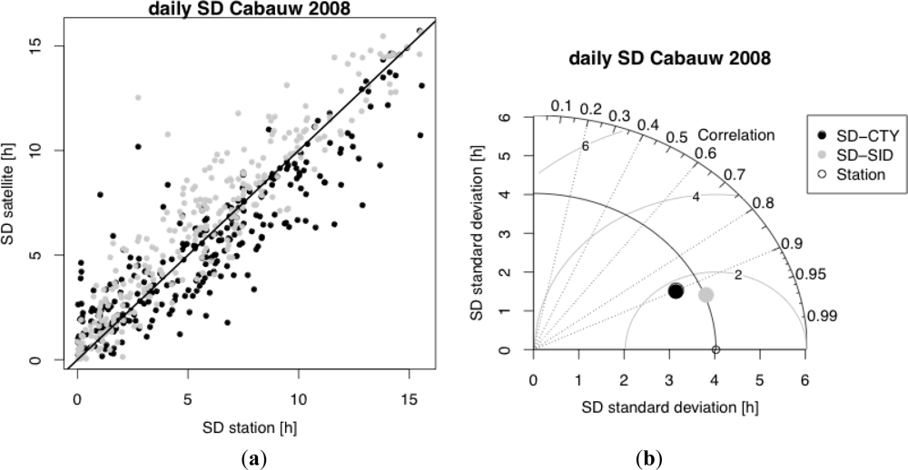
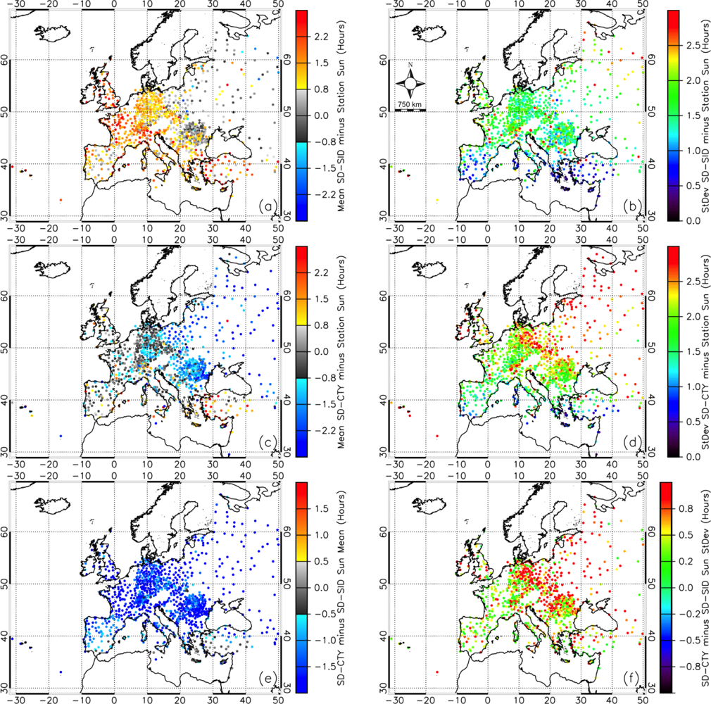
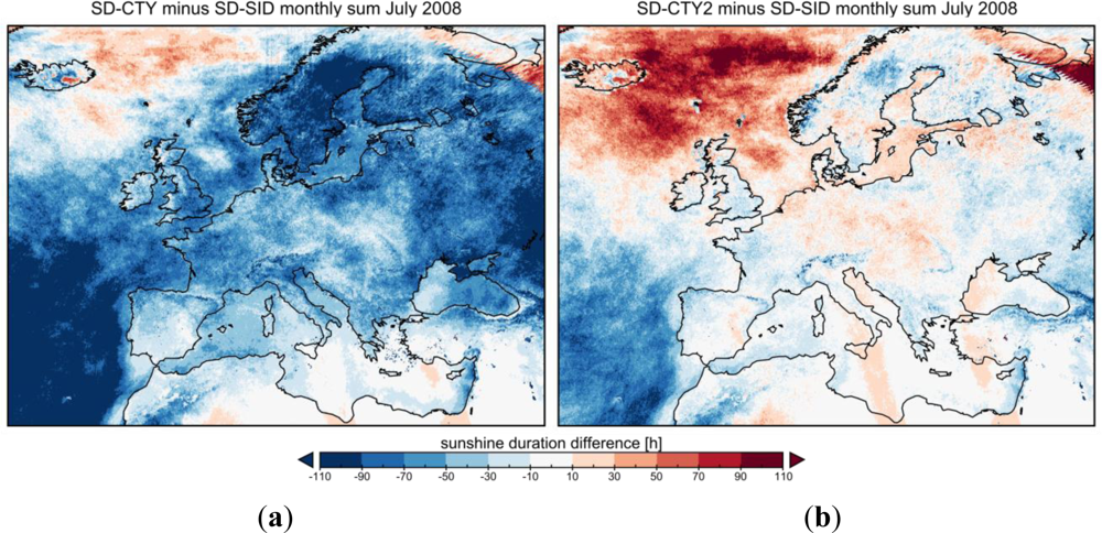
The satellite SD products were intercompared and validated against station measurements over land. This comparison and validation process highlighted some uncertainties in the satellite products. Differences between the products were found to be considerable over ocean regions, sometimes approaching 70%. However, the daily satellite SD products were found to agree well over land with high quality BSRN station data (correlation >90%, RMS difference between 1 to 2 h, mean difference within ±1 h). Both satellite-based SD products also showed good agreement with lower-quality SYNOP station data, where SD-SID mainly overestimated SD and SD-CTY underestimated SD. In this case, the mean daily bias for 2008 across the ∼900 European stations used ranges between −1.6 and 1.4 h (95% within ±1 h) for SD-CTY and −0.5 and 1.7 h (74% within ±1 h) for SD-SID (
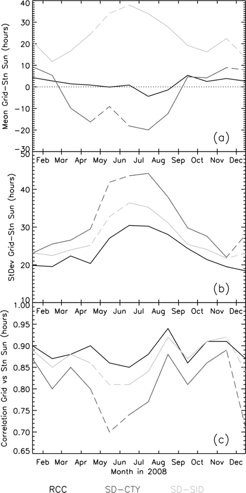
Figure 9). The corresponding standard deviations were between 1.3 and 3.3 h (45% within 2 h) for SD-CTY and 1.2 and 2.5 h (80% within 2 h) for SD-SID. The station-satellite correlations for these daily data are also high, ranging between 0.65 and 0.92 for SD-CTY and 0.77 and 0.95 for SD-SID. Both products exhibited seasonal cycles in the daily agreement with the highest standard deviations observed in summer. The seasonal cycle in the mean daily biases was found to be opposite in sense for each product, with the most positive (negative) biases being observed during the summer for the SD-SID (SD-CTY) product. Overall, the SD-SID product showed the most consistent and stable agreement with the station data, although biases for this method were slightly larger.
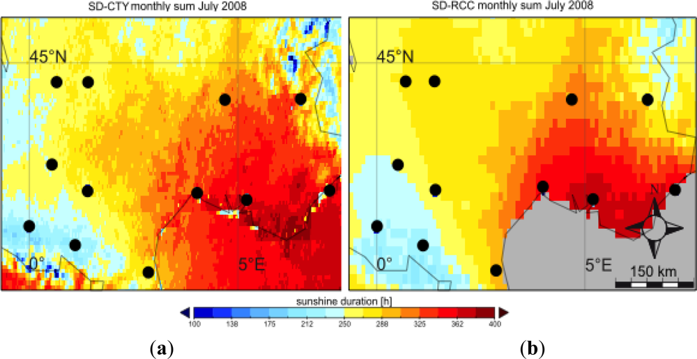
Compared to station-based gridded SD data, it was expected that the satellite-based SD products would perform better, particularly in regions with a sparse station network. Comparison with the monthly 0.1-degree SD-RCC gridded station SD product was limited because the SYNOP stations used to evaluate the product were generally in the same areas as the CLIMAT stations used to generate the SD-RCC product. Thus, the number of SYNOP reference stations in regions with a low density of CLIMAT stations was too low to confirm this assumption in a statistically robust way.
In summary, the satellite-based SD datasets presented in this paper can help to improve the spatial and temporal information of gridded SD datasets. The high spatial resolution offers a variety of possibilities for applications in agriculture, solar technologies, or tourism. Combined with a good accuracy over land, it can also be a basis for scientific studies. Another advantage compared to other gridded state-of-the-art SD datasets is the daily temporal resolution (e.g., SD-RCC is only available on a monthly basis) and availability over ocean regions. However, there are uncertainties in the satellite products and in the interpolated station data, which should be considered in any application. In particular, the uncertainty of the satellite SD products over ocean may be large, but cannot be properly assessed owing to lack of in situ observations in these areas. Besides the unknown uncertainty of the CM SAF CTY product, the uncertainty of the SD-CTY method results mainly from the treatment of fractional clouds whose impact is quite strong. The uncertainty of the SD-SID method results mainly from the SID product, whose accuracy for monthly means is estimated by CM SAF to be better than 15 W/m2[31] (for instantaneous SID values, the uncertainty may be larger). The variation of the SID threshold of ±15 W/m2 showed only minor influences on the retrieval of SD-SID. This leads to the assumption that the overall uncertainty of SD-SID is lower than for SD-CTY.
SD-SID, being superior to SD-CTY, was selected to become an operational product within the Regional Climate Centre on Climate Monitoring. Monthly maps of sums and anomalies will be freely provided in the near future based on CM SAF Near-Real-Time data in an operational mode. CM SAF recently released a Thematic Climate Data Record for SID covering the years 1983–2005. Deriving sunshine duration based on this dataset for the generation of a long-term record, which can be used as reference climatology and for climate studies, has been planned.
It is also conceivable to use other SAF products, such as cloud fractional cover, or cloud optical thickness, to derive a satellite-based SD. However, just as for SID, the basis for these products is the underlying cloud mask. Thus, the accuracy of the resulting SD product is strongly dependent on the accuracy of the cloud mask. Because SD-SID is insensitive to the ±15 W/m2 uncertainty of SID, the cloud mask will be the limiting factor, and it is not expected that products, such as cloud fractional cover or cloud optical thickness, will give better SD estimates. Finally, a very promising option is the merging of satellite data and station data. In this way, the advantages of both methods could be combined.

Acknowledgments

The research leading to these results received funding from Deutscher Wetterdienst (DWD) and the European Union (Seventh Framework Programme (FP7/2007-2013) under grant agreement n° 242093. We are grateful to Richard Müller and Martin Stengel from DWD for the provision of CM SAF data and valuable comments on the draft of the paper. We thank Andrea Kreis (DWD) for assistance with the processing of SYNOP data. The authors acknowledge funding from the Hessian initiative for the development of scientific and economic excellence (LOEWE) at the Biodiversity and Climate Research Centre (BiK-F), Frankfurt/Main.

References

  1. Monteith, J.L. Climate and the efficiency of crop production in Britain. Philos. Trans. R. Soc. Lond 1977, 281, 277–294. [Google Scholar]
  2. Murray, S.J.; Watson, I.M.; Prentice, I.C. The use of dynamic global vegetation models for simulating hydrology and the potential integration of satellite observations integration of satellite observations. Prog. Phys. Geogr. 2013, 37. [Google Scholar] [CrossRef]
  3. Döll, P.; Kaspar, F.; Lehner, B. A global hydrological model for deriving water availability indicators: Model tuning and validation. J. Hydrol 2003, 270, 105–134. [Google Scholar]
  4. Almorox, J.; Hontoria, C. Global solar radiation estimation using sunshine duration in Spain. Energy Convers. Manag 2004, 45, 1529–1535. [Google Scholar]
  5. Ertekin, C.; Evrendilek, F. Spatio-temporal modeling of global solar radiation dynamics as a function of sunshine duration for Turkey. Agric. For. Meteorol 2007, 145, 36–47. [Google Scholar]
  6. Lam, J.C.; Wan, K.K.W.; Lau, C.C.S.; Yang, L. Climatic influences on solar modelling in China. Renew. Energy 2008, 33, 1591–1604. [Google Scholar]
  7. Tang, W.J.; Yang, K.; He, J.; Qin, J. Quality control and estimation of global solar radiation in China. Sol. Energy 2010, 84, 466–475. [Google Scholar]
  8. Tang, W.J.; Yang, K.; Qin, J.; Min, M. Development of a 50-year daily surface solar radiation dataset over China. Sci. China Earth Sci. 2013. [Google Scholar] [CrossRef]
  9. Moradi, I. Quality control of global solar radiation using sunshine duration hours. Energy 2009, 34, 1–6. [Google Scholar]
  10. Wild, M. Enlightening Global Dimming and Brightening. Bull. Amer. Meteor. Soc 2012, 93, 27–37. [Google Scholar]
  11. Sanchez-Lorenzo, A.; Palle, E.; Wild, M.; Calbo, J.; Brunetti, M.; Stanhill, G.; Bradzil, R.; Barriendos, M.; Pereira, P.; Azorin-Molina, C. The SunCloud project: Worldwide compilation of long-term series of sunshine duration and cloudiness observation. Geophys. Res. Abstr. EGU Gen. Assem. 2010, 12. EGU2010-14316. [Google Scholar]
  12. Raichijk, C. Observed trends in sunshine duration over South America. Int. J. Climatol 2012, 32, 669–680. [Google Scholar]
  13. Jhajharia, D.; Singh, V.P. Trends in temperature, diurnal temperature range and sunshine duration in Northeast India. Int. J. Climatol 2011, 31, 1353–1367. [Google Scholar]
  14. Sanchez-Lorenzo, A.; Calbo, J.; Martin-Vide, J. Spatial and Temporal trends in sunshine duration over Western Europe (1938–2004). J. Clim 2008, 21, 6089–6098. [Google Scholar]
  15. World Meteorological Organization (WMO). Guide to Meteorological Instruments and Methods of Observation, 7th ed.; WMO: Geneva, Switzerland, 2008. [Google Scholar]
  16. United Kingdom Met Office. Available online: http://www.metoffice.gov.uk/climate/uk/anomacts/ (accessed on 1 March 2013).
  17. German Meteorological Service DWD. Available online: http://www.dwd.de (accessed on 1 March 2013).
  18. World Meteorological Organization (WMO) Regional Climate Centre on Climate Monitoring. Available online: http://www.dwd.de/rcc-cm (accessed on 1 March 2013).
  19. New, M.; Lister, D.; Hulme, M.; Makin, I. A high-resolution data set of surface climate over global land areas. Clim. Res 2002, 21, 1–25. [Google Scholar]
  20. Dolinar, M. Spatial interpolation of sunshine duration in Slovenia. Meteorol. Appl 2006, 13, 375–384. [Google Scholar]
  21. Hogewind, F.; Bissolli, P. Operational Maps of monthly mean Temperature for WMO-Region VI (Europe and Middle East). Idöjárás, Q. J. Hung. Metereol. Serv 2011, 115, 31–49. [Google Scholar]
  22. Essa, K.S.; Etman, S.M. On the relation between cloud cover amount and sunshine duration. Meteorol. Atmos. Phys 2004, 87, 235–240. [Google Scholar]
  23. Kandirmaz, H.M. A model for the estimation of the daily global sunshine duration from meteorological geostationary satellite data. Int. J. Remote Sens 2006, 27, 5061–5071. [Google Scholar]
  24. Journée, M.; Demain, C.; Bertrand, C. Sunshine duration climate maps of Belgium and Luxembourg based on Meteosat and in-situ observations. Adv. Sci. Res 2013, 10, 15–19. [Google Scholar]
  25. Ångström, A. Solar and terrestrial radiation. Q. J. Roy. Meteor. Soc 1924, 50, 121–125. [Google Scholar]
  26. Good, E. Estimating daily sunshine duration over the UK from geostationary satellite data. Weather 2010, 65, 324–328. [Google Scholar]
  27. CM SAF. Algorithm Theoretical Basis Document; Version 1.0; SAF/CM/DWD/ATBD/CFC_CTH_CTO_SEVIRI; DWD: Offenbach, Germany, 2009. [Google Scholar]
  28. CM SAF. Algorithm Theoretical Basis Document; Version 1.2; SAF/CM/DWD/ATBD/SID; DWD: Offenbach, Germany, 2010. [Google Scholar]
  29. Skartveit, A.; Olseth, J.; Tuft, M. An hourly diffuse fraction model with correction for variability and surface albedo. Sol. Energy 1998, 63, 173–183. [Google Scholar]
  30. Mueller, R.W.; Matsoukas, C.; Gratzki, A.; Behr, H.D.; Hollmann, R. The CM SAF operational scheme for the satellite based retrieval of solar surface irradiance—A LUT based eigenvector hybrid approach. Remote Sens. Environ 2009, 113, 1012–1024. [Google Scholar]
  31. CM SAF. Validation Report Direct Irradiance; Version 1.2; Doc. No: SAF/CM/DWD/VAL/SID; DWD: Offenbach, Germany, 2010. [Google Scholar]
  32. Baseline Surface Radiation Network (BSRN). Available online: http://www.bsrn.awi.de (accessed on 1 March 2013).
  33. Ohmura, A.; Dutton, E.; Forgan, B.; Fröhlich, C.; Gilgen, H.; Hegner, H.; Heimo, A.; König-Langlo, G.; McArthur, B.; Müller, G.; et al. Baseline Surface Radiation Network (BSRN/WCRP): New precision radiometry for climate research. Bull. Amer. Met. Soc 1998, 79, 2115–2136. [Google Scholar]
Figure 1. Differences between the SD-CTY calculated from 15-minute input data and SD-CTY from 1-hourly data for March 2009 (SD-CTY15 minus SD-CTY60).
Remotesensing 05 02943f1
Figure 2. Comparison of frequency distributions for 15-min data and 1-hourly data.
Remotesensing 05 02943f2
Figure 3. SD-CTY (left) and SD-SID (right) for January 2008 (top row), April (second row), July (third row) and October (bottom row).
Remotesensing 05 02943f3
Figure 4. SD-CTY minus SD-SID differences for January (a), April (b), July (c), and October (d) for the year 2008. The panels show relative differences (in percent) in reference to SD-SID.
Remotesensing 05 02943f4
Figure 5. Comparison of daily SD data for SD-CTY and SD-SID with station data for Cabauw (year 2008). The grey circles in the Taylor diagram indicate the root mean square difference.
Remotesensing 05 02943f5
Figure 6. SD-SID (a), SD-RCC (b), and SD-CTY (c) for July 2008. (d) illustrates the positions of the spatial subsets in Figures 6, 7 and 8. In order to show the spatial features, the color bars for SD-SID and SD-CTY are not the same.
Remotesensing 05 02943f6
Figure 7. SD-CTY (a) and for SD-RCC (b) for July 2008. The figures show a sector of about 3° longitude × 8° latitude centered over the south of France.
Remotesensing 05 02943f7
Figure 8. SD-CTY (a) and for SD-RCC (b) for July 2008. The figures show a sector of about 3° longitude × 8° latitude centered over the Balkans.
Remotesensing 05 02943f8
Figure 9. Time series of daily sunshine duration of SEVIRI minus station (a) mean difference and (b) standard deviations of differences. Panel (c) shows the corresponding SEVIRI vs. station correlations. Results are shown for both the SD-CTY (black) and SD-SID (grey) products.
Remotesensing 05 02943f9
Figure 10. Maps showing (a) mean daily SD-SID minus station difference; (b) standard deviation of daily SD-SID minus station differences; (c) mean daily SD-CTY minus station difference; (d) standard deviation of daily SD-CTY minus station differences; (e) mean daily SD-CTY bias minus SD-SID bias (i.e., panel (c) minus panel (a)) and (f) mean daily SD-CTY standard deviation minus SD-SID standard deviation (i.e., panel (d) minus panel (b)) at each station for January 2008.
Remotesensing 05 02943f10
Figure 11. Maps showing (a) mean daily SD-SID minus station difference; (b) standard deviation of daily SD-SID minus station differences; (c) mean daily SD-CTY minus station difference; (d) standard deviation of daily SD-CTY minus station differences; (e) mean daily SD-CTY bias minus SD-SID bias (i.e., panel (c) minus panel (a)) and (f) mean daily SD-CTY standard deviation minus SD-SID standard deviation (i.e., panel (d) minus panel (b)) at each station for July 2008.
Remotesensing 05 02943f11
Figure 12. Annual cycles of gridded product minus non-CLIMAT station sunshine duration monthly (a) mean differences and (b) standard deviation of differences. Panel (c) shows the corresponding correlations. Results are shown for SD-RCC (Black), SD-CTY (dark-grey) and SD-SID (light-grey) products. For information, the unofficial monthly totals for May (5 missing days) and December (9 missing days), are dashed in the plot due to missing values.
Remotesensing 05 02943f12
Figure 13. Annual cycles for the SD-SID product minus station sunshine duration monthly (a) mean differences and (b) standard deviation of differences. Panel (c) shows the corresponding SEVIRI vs. station correlations. Results are shown for validation using all available SYNOPS station data (black) and non-CLIMAT only stations (grey). For information, the unofficial monthly totals for May (five missing days) and December (nine missing days), are dashed in the plot due to missing values.
Remotesensing 05 02943f13
Figure 14. Difference of SD-CTY minus SD-SID (a), and SD-CTY2 minus SD-SID (b) for monthly sums of July 2008. In the retrieval of SD-CTY2 a factor of 0.935 was applied for fractional clouds.
Remotesensing 05 02943f14
Table 1. Solar elevation angle thresholds (degrees) for cloud classes 15, 16, and 17 for each month of 2008. In brackets are the associated explained variances for the linear regression between SIDNorm and the corresponding solar elevation angle.
MonthCTY = 15CTY = 16CTY = 17
January7.9 (0.84)8.4 (0.87)19.7 (0.79)
February8.7 (0.81)9.5 (0.86)19 (0.51)
March9.8 (0.81)10.2 (0.87)20 (0.53)
April11.2 (0.79)11.9 (0.86)23.8 (0.58)
May13.4 (0.80)14.6 (0.85)29.4 (0.62)
June14.7 (0.7914.6 (0.89)31.3 (0.65)
July15.2 (0.78)14.6 (0.91)31 (0.62)
August13.4 (0.80)13.4 (0.92)26.3 (0.60)
September11.5 (0.80)12.8 (0.84)23.8 (0.53)
October9.7 (0.82)11.4 (0.82)22.3 (0.53)
November8.4 (0.84)8.8 (0.85)21.6 (0.77)
December7.6 (0.84)7.6 (0.85)18.1 (0.81)
Table 2. Mean, standard deviation, and mean difference relative to the 120 W/m2 SD product, for the SD-SID product with three different thresholds. The results correspond to monthly totals from 2008.
SIDNormThreshold (W/m2)Mean Monthly SD Total (Hours)Standard Deviation (Hours)Mean (Test Product minus 120 W/m2 SD Product) (Hours)
120214.2598.80
135211.2299.0−3.03
105217.5298.63.27
Table 3. Mean, standard deviation, and mean difference relative to the other temporal resolution, for the SD-CTY and SD-SID products with 15-minute and 1-hourly bases. The results are calculated for monthly totals from March 2009 for SD-CTY, and August 2007 for SD-SID over the whole domain.
ProductMean (Hours)Standard Deviation (Hours)Mean Difference (Hours)
SD-CTY15162.5873.82−0.55
SD-CTY60163.1373.960.55
SD-SID15298.3466.500.43
SD-SID60297.9166.94−0.43
Table 4. Comparison of daily SD data for SD-CTY, SD-SID, and station data. Shown are the Pearson’s correlation (cor), the mean difference satellite product minus station (md), and the ratio of the satellite product to station standard deviations (sdr). To estimate the influence of the annual cycle on cor, the ratio of the explained variances for a sine curve and for the satellite product are given in brackets (for details see Section 4.2).
CabauwCarpentrasPayerneToravereLindenberg
cor SD-CTY0.90 (0.16)0.94 (0.16)0.92 (0.17)0.90 (0.28)0.92 (0.25)
cor SD-SID0.94 (0.15)0.95 (0.16)0.93 (0.16)0.95 (0.25)0.96 (0.23)
md SD-CTY−0.29−0.39−0.04−1.00−0.43
md SD-SID0.750.420.940.291.08
sdr SD-CTY0.871.081.081.161.14
sdr SD-SID1.011.061.010.940.96
Table 5. Grid box minus station SD validation statistics for the SD-RCC product for 2008 (monthly totals) using non-CLIMAT stations for validation. The table shows results for mean monthly bias (for each station) vs. elevation and mean monthly bias vs. the distance to the nearest CLIMAT station for that SD-RCC grid box (DNC). “Slope” denotes the gradient of the linear regression line fitted to the data. “r” denotes Pearson correlation coefficient. Results shown in parentheses are insignificant at the 5% level. The number of stations used in the analysis varies between 616 (January) and 800 (July).
MonthBias vs. Elev.Bias vs. DNC

Slope (h·m−1)rSlope (h·deg−1)r
January0.00550.14(0.9646)(0.03)
February0.00880.223.02370.09
March0.00690.142.80680.07
April0.00500.12(−2.2011)(−0.06)
May(0.0041)(0.07)−5.2150−0.11
June0.00750.12(−1.3737)(−0.03)
July0.01310.21(−1.6880)(−0.03)
August0.01280.22(−1.6004)(−0.03)
September0.00970.205.52330.21
October0.00820.193.33280.09
November0.00820.211.83780.07
December0.00590.16(−1.6560)(−0.06)

