Retrieval of Forest Aboveground Biomass and Stem Volume with Airborne Scanning LiDAR

 ,
, 

Abstract
:1. Introduction
2. Materials and Methods
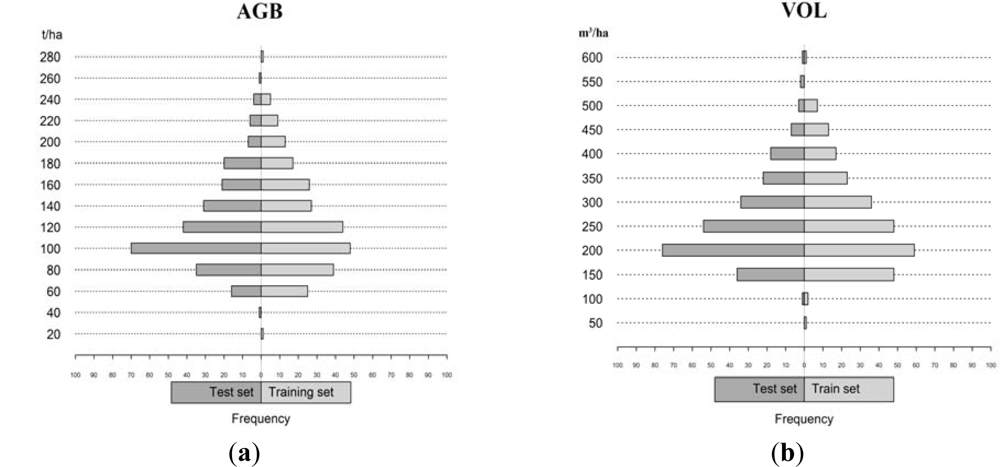
2.1. Study Area and Field Data
2.2. Calculation of AGB
2.3. Tree Analyses for Evaluating the Biomass Models Used
2.4. LiDAR Data
2.5. Individual Tree Detection
2.5.1. Automatic Tree Detection and Visual Interpretation
2.5.2. Retrieval of AGB and VOL from Individual Tree Detection
2.6. Area-Based Approach
2.7. Statistical Analyses
3. Results
3.1. Validation of the Biomass Estimation Models Used
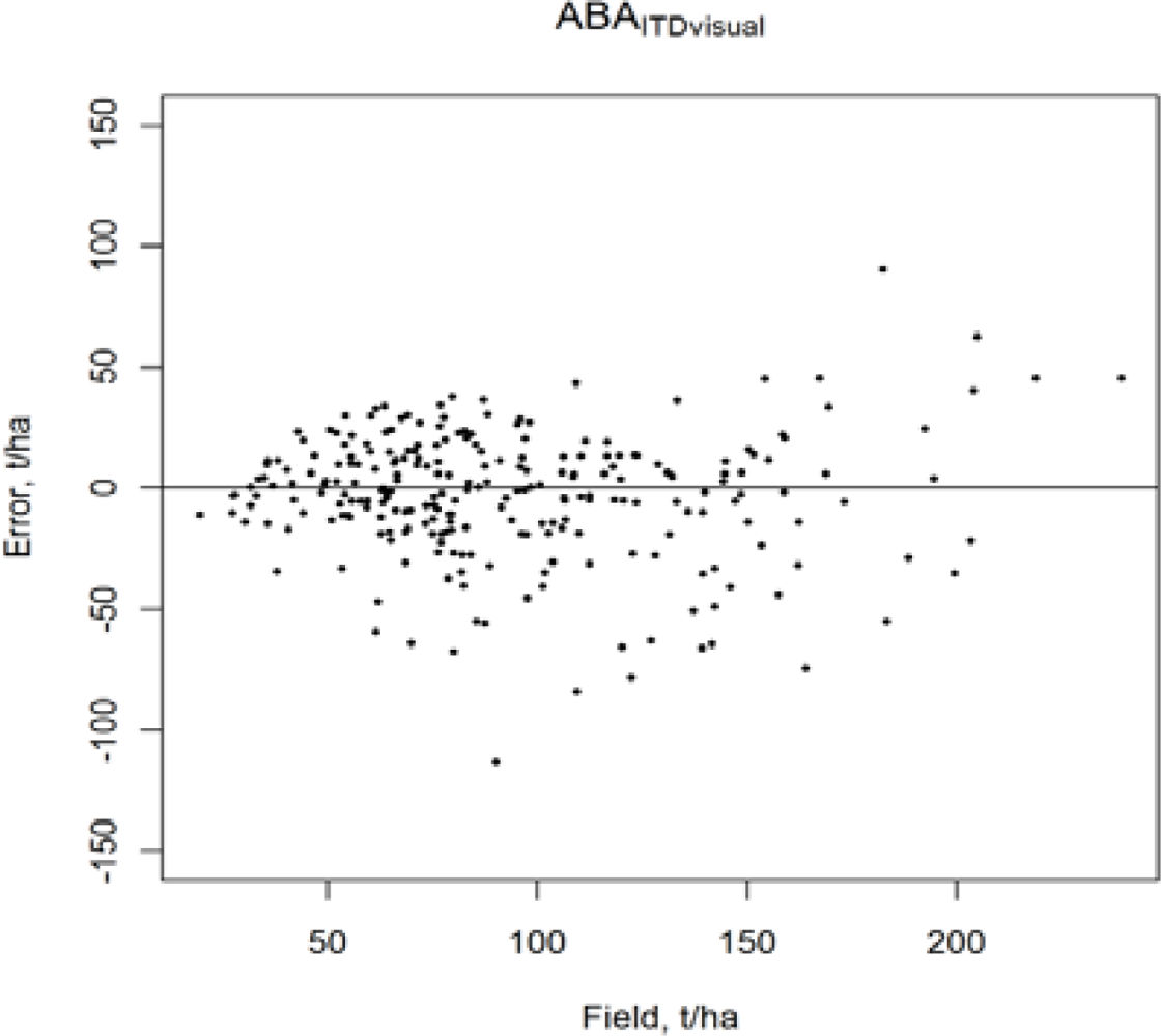
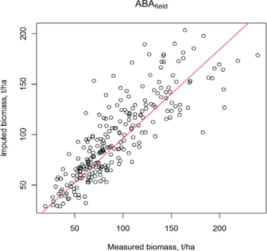
3.2. Accuracy of the ABA
4. Discussion
5. Conclusions
Acknowledgments
- Conflict of InterestThe authors declare no conflict of interest.
References
- Vastaranta, M.; Kankare, V.; Holopainen, M.; Yu, X.; Hyyppä, J.; Hyyppä, H. Combination of individual tree detection and area-based methodology in imputation of forest variables using airborne laser data. ISPRS J. Photogram. 2012, 67, 73–79. [Google Scholar]
- Kellndorfer, J.M.; Walker, W.S.; LaPoint, E.; Kirsch, K.; Bishop, J.; Fiske, G. Statistical fusion of LiDAR, InSAR, and optical remote sensing data for forest stand height characterization: A regional-scale method based on LVIS, SRTM, Landsat ETM+, and ancillary data sets. J. Geophys. Res. 2010, 115. [Google Scholar] [CrossRef]
- Næsset, E. Determination of mean tree height of forest stands using airborne laser scanner data. ISPRS J. Photogram. 1997, 52, 49–56. [Google Scholar]
- Hyyppä, J.; Inkinen, M. Detecting and estimating attributes for single trees using laser scanner. Photogramm. J. Fin. 1999, 16, 27–42. [Google Scholar]
- Koch, B. Status and future of laser scanning, synthetic aperture radar and hyperspectral remote sensing data for forest biomass assessment. ISPRS J. Photogram. 2010, 65, 581–590. [Google Scholar]
- Holopainen, M.; Hyyppä, J.; Vaario, L.-M.; Yrjälä, K. Implications of Technological Development to Forestry. In Forest and Society—Responding to Global Drivers of Change; Mery, G., Katila, P., Galloway, G., Alfaro, R.I., Kanninen, M., Lobovikov, M., Varjo, J., Eds.; IUFRO-World Series: Vienna, Austria, 2010; pp. 157–182. [Google Scholar]
- Falkowski, M.; Smith, A.; Hudak, A.; Gessler, P.; Vierling, L.; Crookston, N. Automated estimation of individual conifer tree height and crown diameter via two-dimensional spatial wavelet analysis of LiDAR data. Can. J. Remote Sens. 2006, 32, 153–161. [Google Scholar]
- Magnussen, S.; Eggermont, P.; LaRiccia, V.N. Recovering tree heights from airborne laser scanner data. For. Sci. 1999, 45, 407–422. [Google Scholar]
- Maltamo, M.; Mustonen, K.; Hyyppä, J.; Pitkänen, J.; Yu, X. The accuracy of estimating individual tree variables with airborne laser scanning in a boreal nature reserve. Can. J. For. Res. 2004, 34, 1791–1801. [Google Scholar]
- Hyyppä, J.; Kelle, O.; Lehikoinen, M.; Inkinen, M. A segmentation-based method to retrieve stem volume estimates from 3-dimensional tree height models produced by laser scanner. IEEE Trans. Geosci. Remote Sens. 2001, 39, 969–975. [Google Scholar]
- Wallerman, J.; Holmgren, J. Remote sensing based imputation of sample plot data for forest management planning utilizing single-tree forecast models. Remote Sens. Environ. 2007, 110, 501–508. [Google Scholar]
- Lefsky, M.A.; Harding, D.; Cohen, W.B.; Parker, G.; Shugart, H.H. Surface lidar remote sensing of basal area and biomass in deciduous forests of Eastern Maryland, USA. Remote Sens. Environ. 1999, 67, 83–98. [Google Scholar]
- Means, J.E.; Acker, S.A.; Fitt, B.J.; Renslow, M.; Emerson, L.; Hendrix, C.J. Predicting forest stand characteristics with airborne scanning lidar. Photogramm. Eng. Remote Sensing 2000, 66, 1367–1371. [Google Scholar]
- Næsset, E. Predicting forest stand characteristics with airborne scanning laser using a practical two-stage procedure and field data. Remote Sen. Environ. 2002, 80, 88–99. [Google Scholar]
- Van Aardt, J.A.N.; Wynne, R.H.; Scrivani, J.A. Lidar-based mapping of forest volume and biomass by taxonomic group using structurally homogenous segments. Photogramm. Eng. Remote Sensing 2008, 74, 1033–1044. [Google Scholar]
- Brandtberg, T. Classifying individual tree species under leaf-off and leaf-on conditions using airborne lidar. ISPRS J. Photogram. 2009, 61, 325–340. [Google Scholar]
- Holmgren, J.; Persson, Å. Identifying species of individual trees using airborne laser scanner. Remote Sens. Environ. 2004, 90, 415–550. [Google Scholar]
- Korpela, I.; Ørka, H.O.; Maltamo, M.; Tokola, T.; Hyyppä, J. Tree species classification using airborne LiDAR—Effects of stand and tree parameters, downsizing of training set, intensity normalization, and sensor type. Silva Fenn. 2010, 44, 319–339. [Google Scholar]
- Vauhkonen, J.; Korpela, I.; Maltamo, M.; Tokola, T. Imputation of single-tree attributes using airborne laser scanning-based height, intensity, and alpha shape metrics. Remote Sens. Environ 2010, 114, 1263–1276. [Google Scholar]
- Solberg, S.; Næsset, E.; Hanssen, K.H.; Cristiansen, E. Mapping defoliation during a severe insect attack on Scots pine using airborne laser scanning. Remote Sens. Environ. 2006, 102, 384–376. [Google Scholar]
- Solberg, S.; Næsset, E. Monitoring Forest Health by Remote Sensing. Proceedings of Symposium on Forests in a Changing Environment—Results of 20 years ICP Forests Monitoring, Göttingen, Germany, 25–28 October 2006; Schriftenreihe der Forstlichen Fakultät Göttingen und der Nordwestdeutschen Forstlichen Versuchsanstalt: Göttingen, Germany, 2007; pp. 99–104. [Google Scholar]
- Kantola, T.; Vastaranta, M.; Yu, X.; Lyytikäinen-Saarenmaa, P.; Holopainen, M.; Talvitie, M.; Kaasalainen, S.; Solberg, S.; Hyyppä, J. Classification of defoliated trees using tree-level airborne laser scanning data combined with aerial images. Remote Sens. 2010, 2, 2665–2679. [Google Scholar]
- Solberg, S. Mapping gap fraction, LAI and defoliation using various ALS penetration variables. Int. J. Remote Sens. 2010, 32, 1227–1244. [Google Scholar]
- Vastaranta, M.; Holopainen, M.; Yu, X.; Haapanen, R.; Melkas, T.; Hyyppä, J.; Hyyppä, H. Individual tree detection and area-based approach in retrieval of forest inventory characteristics from low-pulse airborne laser scanning data. Photogram. J. Fin. 2011, 22, 1–13. [Google Scholar]
- Solberg, S.; Brunner, A.; Hanssen, K.H.; Lange, H.; Næsset, E.; Rautiainen, M.; Stenberg, P. Mapping LAI in a Norway spruce forest using airborne laser scanning. Remote Sens. Environ. 2009, 113, 2317–2327. [Google Scholar]
- Solberg, S. Mapping gap fraction, LAI and defoliation using various ALS penetration variables. Int. J. Remote Sens. 2008, 31, 1227–1244. [Google Scholar]
- Korhonen, L.; Korpela, I.; Heiskanen, J.; Maltamo, M. Airborne discrete-return LIDAR data in the estimation of vertical canopy cover, angular canopy closure and leaf area index. Remote Sens. Environ. 2011, 115, 1065–1080. [Google Scholar]
- Popescu, S.C.; Wynne, R.H.; Nelson, R.F. Measuring individual tree crown diameter with lidar and assessing its influence on estimation forest volume and biomass. Can. J. Remote Sens. 2003, 29, 564–577. [Google Scholar]
- Popescu, S.C.; Wynne, R.H.; Scrivani, J.A. Fusion of small-footprint lidar and multispectral data to estimate plot-level volume and biomass in deciduous and pine forests in Virginia, USA. For. Sci. 2004, 50, 551–565. [Google Scholar]
- Bortolot, Z.; Wynne, R.H. Estimating forest biomass using small footprint LiDAR data: An individual tree-based approach that incorporates training data. ISPRS J. Photogramm. 2005, 59, 342–360. [Google Scholar]
- Van Aardt, J.A.N.; Wynne, R.H.; Oderwald, R.G. Forest volume and biomass estimation using small-footprint lidar distributional parameters on a per-segment basis. For. Sci. 2006, 52, 636–649. [Google Scholar]
- Næsset, E. Estimation of above- and below-ground biomass in boreal forest ecosystems. Int. Arch. Photogramm. Remote Sens. Spat. Inf. Sci. 2004, 36, 145–148. [Google Scholar]
- Jochem, A.; Hollaus, M.; Rutzinger, M.; Höfle, B. Estimation of aboveground biomass in Alpine forests: A semi-empirical approach considering canopy transparency derived from airborne LiDAR data. Sensors 2011, 11, 278–295. [Google Scholar]
- Latifi, H.; Nothdurft, A.; Koch, B. Non-parametric prediction and mapping of standing timber volume and biomass in a temperate forest: Application of multiple optical/LiDAR-derived predictors. Forestry 2010, 83, 395–407. [Google Scholar]
- Breidenbach, J.; Næsset, E.; Lien, V.; Gobakken, T.; Solberg, S. Prediction of species specific forest inventory attributes using a nonparametric semi-individual tree crown approach based on fused airborne laser scanning and multispectral data. Remote Sens. Environ. 2010, 114, 911–924. [Google Scholar]
- Breidenbach, J.; Næsset, E.; Gobakken, T. Improving k-nearest neighbor predictions in forest inventories by combining high and low density airborne laser scanning data. Remote Sens. Environ. 2012, 117, 358–365. [Google Scholar]
- Tuominen, S. Personal Communication. 2013.
- Holopainen, M.; Haapanen, R.; Tuominen, S; Viitala, R. Performance of Airborne Laser Scanning- and Aerial Photograph-Based Statistical and Textural Features in Forest Variable Estimation. Proceedings of SilviLaser 2008: 8th International Conference on LiDAR Applications in Forest Assessment and Inventory, Edinburgh, UK, 17–19 September 2008; pp. 105–112.
- Vastaranta, M.; Holopainen, M.; Haapanen, R.; Yu, X.; Melkas, T.; Hyyppä, J.; Hyyppä, H. Comparison between an Area-based and Individual Tree Detection Method for Low-pulse Density Als-based Forest Inventory. Proceedings of Laser Scanning, Paris, France, 1–2 September 2009; pp. 147–151.
- Rasinmäki, J.; Kalliovirta, J.; Mäkinen, A. An adaptable simulation framework for multiscale forest resource data. Comput. Electron. Agr. 2009, 66, 76–84. [Google Scholar]
- Repola, J. Biomass equations for birch in Finland. Silva Fenn. 2008, 42, 605–624. [Google Scholar]
- Repola, J. Biomass equations for Scots pine and Norway spruce in Finland. Silva Fenn. 2009, 43, 625–647. [Google Scholar]
- Laasasenaho, J. Taper curve and volume functions for pine, spruce and birch. Commun. Inst. For. Fenn. 1982, 108, 74. [Google Scholar]
- Kankare, V.; Holopainen, M.; Vastaranta, M.; Puttonen, E.; Yu, X.; Hyyppä, J.; Vaaja, M.; Hyyppä, H.; Alho, P. Individual tree biomass estimation using terrestrial laser scanning. ISPRS J. Photogram. 2013, 75, 64–75. [Google Scholar]
- Chandra, S.; Sivaswamy, J. An Analyses of Curvature based Ridge and Valley Detection. Proceedings of International Conference on Acoustics, Speech and Signal Processing, Toulouse, France, 14–19 May 2006; pp. 737–740.
- Yu, X.; Hyyppä, J.; Vastaranta, M.; Holopainen, M.; Viitala, R. Predicting individual tree attributes from airborne laser point clouds based on random forests technique. ISPRS J. Photogram. 2011, 66, 28–37. [Google Scholar]
- Mathworks. Image Processing Toolbox. 2010. Available online: http://www.mathworks.se/help/images/examples/marker-controlled-watershed-segmentation.html (accessed on 2 June 2012).
- Kalliovirta, J.; Tokola, T. Functions for estimating stem diameter and tree age using tree height, crown width and existing stand database information. Silva Fenn. 2005, 39, 227–248. [Google Scholar]
- Magnussen, S.; Boudewyn, P. Derivations of stand heights from airborne laser scanner data with canopy-based quantile estimators. Can. J. For. Res. 1998, 28, 1016–1031. [Google Scholar]
- Moeur, M.; Stage, A.R. Most similar neighbor: An improved sampling inference procedure for natural resource planning. For. Sci. 1995, 41, 337–359. [Google Scholar]
- Crookston, N.; Finley, A. yaImpute: An R Package for k-NN Imputation. J. Stat. Softw. 2008, 23, 1–16. [Google Scholar]
- Tibshirani, R. Regression shrinkage and selection via the lasso. J. Royal Stat. Soc. B Stat. Meth. 1996, 58, 267–288. [Google Scholar]
- Friedman, J.; Hastie, T.; Tibshirani, R. Regularization paths for generalized linear models via coordinate descent. J. Stat. Softw. 2010, 33, 1–22. [Google Scholar]
- R Development Core Team. R: A Language and Environment for Statistical Computing. R Foundation for Statistical Computing. 2011. Available online: http://www.R-project.org/ (accessed on 1 September 2011).
- Nelson, R.; Krabill, W.; Tonelli, J. Estimating forest biomass and volume using airborne laser data. Remote Sens. Environ. 1988, 24, 247–267. [Google Scholar]
- Lim, K.S.; Treitz, P.M. Estimation of above ground forest biomass from airborne discrete return laser scanner data using canopy-based quantile estimators. Scand. J. For. Res. 2004, 19, 558–570. [Google Scholar]
- Kaartinen, H.; Hyyppä, J. EuroSDR/ISPRS Project, Commission II “Tree Extraction”; Final Report; EuroSDR Official Publication No. 53; European Spatial Data Research: Dublin, Ireland, 2008. [Google Scholar]
- Vastaranta, M.; Holopainen, M.; Yu, X.; Hyyppä, J.; Mäkinen, A.; Rasinmäki, J.; Melkas, T.; Kaartinen, H.; Hyyppä, H. Effects of ALS individual tree detection error sources on forest management planning calculations. Remote Sens. 2011, 3, 1614–1626. [Google Scholar]
- Yu, X.; Hyyppä, J.; Vastaranta, M.; Holopainen, M. Predicting individual tree attributes from airborne laser point clouds based on random forest technique. ISPRS J. Photogram. 2011, 66, 28. [Google Scholar]


| Variable | Tree Species | ||
|---|---|---|---|
| Scots Pine | Norway Spruce | Birch | |
| b0 | −3.198 | −1.808 | −3.654 |
| b1 | 9.547 | 9.482 | 10.582 |
| b2 | 3.241 | 0.469 | 3.018 |
| var(uk) | 0.009 | 0.006 | 0.00068 |
| var(eki) | 0.01 | 0.013 | 0.00727 |
| Data set | n | Variable | Min | Max | Mean | Std |
|---|---|---|---|---|---|---|
| Test | 254 | VOL, m3/ha | 43.6 | 533.3 | 183.4 | 89.5 |
| Test | 254 | Dg, cm | 11.1 | 62.2 | 24.0 | 8.4 |
| Test | 254 | Hg, m | 7.9 | 31.7 | 19.1 | 4.7 |
| Test | 254 | AGB, t/ha | 19.5 | 239.3 | 92.6 | 41.7 |
| Training | 255 | VOL, m3/ha | 46.8 | 586.2 | 189.2 | 99.3 |
| Training | 255 | Dg, cm | 10.0 | 49.8 | 23.7 | 7.3 |
| Training | 255 | Hg, m | 8.2 | 30.9 | 19.1 | 4.6 |
| Training | 255 | AGB, t/ha | 22.4 | 270.8 | 96.2 | 47.5 |
| Scots Pine | Norway Spruce | |||||
|---|---|---|---|---|---|---|
| Mean | Std | Range | Mean | Std | Range | |
| DBH, cm | 19.6 | 4.0 | 15.6 | 20.9 | 7.0 | 26.6 |
| Height, m | 18.8 | 2.4 | 9 | 19.2 | 6.4 | 20 |
| Age, year | 49 | 5 | 16 | 68.6 | 25.8 | 88 |
| Crown ratio | 0.57 | 0.08 | 0.30 | 0.25 | 0.11 | 0.35 |
| Liv. branch, kg | 46 | 25 | 91 | 106 | 69 | 279 |
| Dead branch, kg | 4.2 | 3.3 | 13 | 4.0 | 4.5 | 16 |
| Stem mass, kg | 270 | 122 | 446 | 338 | 281 | 1034 |
| Total mass, kg | 321 | 146 | 541 | 448 | 351 | 1332 |
| Feature | ABAfield | ABAITDauto | ABAITDvisual |
|---|---|---|---|
| Hmax | ● | ● | ● |
| Hstd | ● | ||
| CV | ● | ||
| h10 | ● | ● | |
| h20 | ● | ||
| h30 | ● | ● | |
| h40 | ● | ||
| h50 | ● | ● | |
| h60 | ● | ● | |
| h90 | ● | ||
| p10 | ● | ● | ● |
| p30 | ● | ||
| p40 | ● | ● | |
| p50 | ● | ||
| p70 | ● | ● | |
| p80 | ● | ● | |
| p90 | ● | ● |
| Method | Variable | Bias | Bias (%) | RMSE | RMSE (%) |
|---|---|---|---|---|---|
| ABAfield | AGB, t/ha | −3.2 | −3.5 | 23.0 | 24.9 |
| ABAITDauto | AGB, t/ha | −12.9 | −13.9 | 32.3 | 34.9 |
| ABAITDvisual | AGB, t/ha | −2.8 | −3.1 | 26.4 | 28.5 |
| ABAfield | VOL, m3/ha | −4.9 | −2.7 | 48.4 | 26.4 |
| ABAITDauto | VOL, m3/ha | −22.9 | −12.5 | 62.4 | 34.0 |
| ABAITDvisual | VOL, m3/ha | −3.4 | −1.9 | 53.6 | 29.2 |
| Method | Tree Species | n | Adjusted R2 |
|---|---|---|---|
| ABAfield | Scots pine | 144 | 0.73 |
| ABAfield | Norway spruce | 68 | 0.68 |
| ABAfield | Deciduous trees | 42 | 0.72 |
| ABAfield | All | 254 | 0.71 |
| ABAITDauto | Scots pine | 144 | 0.75 |
| ABAITDauto | Norway spruce | 68 | 0.68 |
| ABAITDauto | Deciduous trees | 42 | 0.71 |
| ABAITDauto | All | 254 | 0.71 |
| ABAITDvisual | Scots pine | 144 | 0.76 |
| ABAITDvisual | Norway spruce | 68 | 0.69 |
| ABAITDvisual | Deciduous trees | 42 | 0.71 |
| ABAITDvisual | All | 254 | 0.72 |
© 2013 by the authors; licensee MDPI, Basel, Switzerland This article is an open access article distributed under the terms and conditions of the Creative Commons Attribution license ( http://creativecommons.org/licenses/by/3.0/).
Share and Cite
Kankare, V.; Vastaranta, M.; Holopainen, M.; Räty, M.; Yu, X.; Hyyppä, J.; Hyyppä, H.; Alho, P.; Viitala, R. Retrieval of Forest Aboveground Biomass and Stem Volume with Airborne Scanning LiDAR. Remote Sens. 2013, 5, 2257-2274. https://doi.org/10.3390/rs5052257
Kankare V, Vastaranta M, Holopainen M, Räty M, Yu X, Hyyppä J, Hyyppä H, Alho P, Viitala R. Retrieval of Forest Aboveground Biomass and Stem Volume with Airborne Scanning LiDAR. Remote Sensing. 2013; 5(5):2257-2274. https://doi.org/10.3390/rs5052257
Chicago/Turabian StyleKankare, Ville, Mikko Vastaranta, Markus Holopainen, Minna Räty, Xiaowei Yu, Juha Hyyppä, Hannu Hyyppä, Petteri Alho, and Risto Viitala. 2013. "Retrieval of Forest Aboveground Biomass and Stem Volume with Airborne Scanning LiDAR" Remote Sensing 5, no. 5: 2257-2274. https://doi.org/10.3390/rs5052257
APA StyleKankare, V., Vastaranta, M., Holopainen, M., Räty, M., Yu, X., Hyyppä, J., Hyyppä, H., Alho, P., & Viitala, R. (2013). Retrieval of Forest Aboveground Biomass and Stem Volume with Airborne Scanning LiDAR. Remote Sensing, 5(5), 2257-2274. https://doi.org/10.3390/rs5052257