Article

SAR Images Statistical Modeling and Classification Based on the Mixture of Alpha-Stable Distributions

1
Signal Processing Laboratory, School of Electronic Information, Wuhan University, Wuhan 430072, China
2
Wireless Communication and Sensor Network Laboratory, School of Electronic Information, Wuhan University, Wuhan 430072, China
*
Author to whom correspondence should be addressed.
Remote Sens. 2013, 5(5), 2145-2163; https://doi.org/10.3390/rs5052145
Submission received: 14 March 2013 / Revised: 23 April 2013 / Accepted: 24 April 2013 / Published: 3 May 2013

Abstract

:
This paper proposes the mixture of Alpha-stable (MAS) distributions for modeling statistical property of Synthetic Aperture Radar (SAR) images in a supervised Markovian classification algorithm. Our work is motivated by the fact that natural scenes consist of various reflectors with different types that are typically concentrated within a small area, and SAR images generally exhibit sharp peaks, heavy tails, and even multimodal statistical property, especially at high resolution. Unimodal distributions do not fit such statistical property well, and thus a multimodal approach is necessary. Driven by the multimodality and impulsiveness of high resolution SAR images histogram, we utilize the mixture of Alpha-stable distributions to describe such characteristics. A pseudo-simulated annealing (PSA) estimator based on Markov chain Monte Carlo (MCMC) is present to efficiently estimate model parameters of the mixture of Alpha-stable distributions. To validate the proposed PSA estimator, we apply it to simulated data and compare its performance to that of a state-of-the-art estimator. Finally, we exploit the MAS distributions and a Markovian context for SAR images classification. The effectiveness of the proposed classifier is demonstrated by experiments on TerraSAR-X images, which verifies the validity of the MAS distributions for modeling and classification of SAR images.

1. Introduction

Synthetic aperture radar (SAR) works in the microwave band and has the ability to operate under all weather conditions. SAR images have been increasingly used in different areas [13]. One fundamental technique for interpretation of SAR images is classification, which is of great importance for land planning, natural risk prevention, target recognition, etc. However, SAR image classification is still a tough work due to the existence of intense speckle. Different classification approaches have been considered in both supervised and unsupervised contexts, based on Markov random field [4], neural networks [5] and other methods [6]. We focus on supervised classification of SAR images based on its statistical property in Markovian framework, in which a proper statistical distribution must be adopted to model SAR images data.
SAR images generally exhibit heavy-tailed and sharp-peaked statistical properties. Many distributions, e.g., Gamma ([7]; Chapter 4), Weibull [8,9], Log-normal ([7]; Chapter 5), [10], K [11,12], generalized Gamma [13], Fisher [14], G0 [15], Alpha-stable and heavy-tailed Rayleigh [16,17], and recently proposed HG0 [18], have been applied to the statistical modeling of SAR images. Gao [19] summarizes the development history and the current researching state of statistical modeling and discusses relevant issues in his work. However, as the resolution of the images increases, multimodal statistical properties become apparent due to the different types of backscatter from a single class. For instance, in an SAR image, building areas contain strong reflectors, textures, and shadows. In this case, the previously mentioned unimodal distributions fail to capture such multimodal statistical properties. Thus, a model with the ability to describe these attributes, as well as a heavy tail and sharp peak, is necessary. Alpha-stable distribution is a flexible model that can fit many other distributions into it. The appeal of Alpha-stable distribution also derives from theoretical reason, which states that stable processes arise as limiting processes of sums of independent identically distributed (i.i.d.) random variables via the generalized central limit theorem. Actually, the only possible nontrivial limit of normalized sums of i.i.d. terms is Alpha-stable. Moreover, Alpha-stable distribution has been used as a successful alternative for modeling non-Gaussian data and has also been applied to understand SAR images, e.g., for image restoration [17], object detection [20,21], image classification [22], and image fusion [23]. Applications of Alpha-stable distribution in other areas such as watermark detection, network traffic and stock returns have also been reported [2426]. Driven by the multimodal and impulsive histogram of high resolution SAR image, as well as the theoretical appeal and successful applications of Alpha-stable family itself, we take the mixture of Alpha-stable distributions that can fit any situation for the statistical modeling of high resolution SAR images.
The main challenge in applying MAS distributions comes from the parameter estimation, as there is no analytical expression for the probability density function. Work on MAS distributions in the literature is very limited: Salas-Gonzalez and Kuruoglu [27] proposed a reversible jump Markov chain Monte Carlo (MCMC) method for MAS distributions with an unknown number of components in the Bayesian frame, but their estimations suffered from large deviations. The same authors introduced an estimator for a mixture of symmetric alpha-stable distributions with identical characteristic exponent for each component [28], and also an estimator for a mixture of skewed alpha-stable distributions with identical shape parameters for each component [29]. In both cases, they considered the number of components to be unknown. Using Buckle’s work [30] on the estimation of distribution parameters, Casarin [31] introduced a random auxiliary vector for MAS distributions with a fixed number of components. However, the algorithm necessary for this approach makes it difficult to draw samples for the auxiliary variable and is time consuming.
In this paper, we introduce a pseudo-simulated annealing (PSA) estimator for the MAS distributions. Experimental results on simulated data show that the PSA estimator obtains accurate parameter values for MAS distributions. We utilize the MAS distributions estimated by PSA for the statistical modeling and classification of SAR images. To verify the effectiveness of the mixture model, classification experiments are carried out using TerraSAR-X data. The supervised Bayesian maximum a posteriori (MAP) classifier is selected over MAS distributions in a Markov random field (MRF) framework. SAR images are represented by MAS distributions that are trained via the PSA estimator and appear as likelihood probabilities. In order to preserve spatial coherence, the MRF introduces prior information, which builds a restraint between pixels and their neighborhoods. The classification is then the solution to the maximization problem of the posterior probability. To solve this problem, we use the Graph Cuts method [3234] to obtain a global optimization. The proposed classifier is validated using TerraSAR-X images.
The remainder of this paper is organized as follows. Section 2 introduces MAS distributions and the PSA estimator. Section 3 gives an explanation of the statistical modeling of SAR images, and Section 4 introduces the MAS-based MRF classification algorithm. Our experiments and results are presented in Section 5, and we summarize the conclusions in Section 6.

2. Mixture of Alpha-Stable Distributions

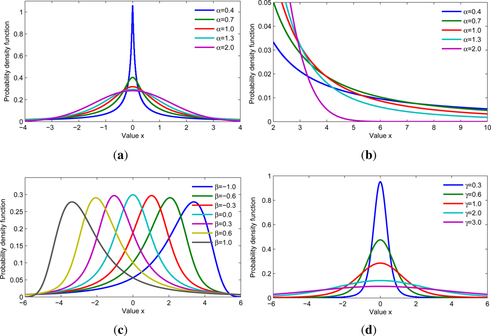
2.1. Alpha-Stable Distribution

The notion of stability was introduced by Levy [35] in his study of normalized sums of independent and identically distributed terms. Due to the lack of an analytical expression for the probability density function (PDF), Alpha-stable distributions are usually described in terms of the characteristic function as
ϕ ( ω ) = { exp { j μ ω | γ ω | α [ 1 j sgn ( ω ) β tan ( π α 2 ] } ) , α 1 exp { j μ ω | γ ω | [ 1 + j sgn ( ω ) β 2 π ln ( ω ) ] } ) , α = 1
where j = 1, “sgn” is the sign function. The four parameters of Alpha-stable distribution are α ∈ (0, 2], β ∈ [−1, 1], γ ∈ ℝ+ and μ ∈ ℝ, representing the characteristic exponent, skewness parameter, dispersion parameter, and location parameter, respectively. The parameter α sets the level of impulsiveness (smaller α gives a more picked PDF and a heavier tail); the parameter β controls the skewness of the PDF (symmetric if β = 0, negatively skewed if β = −1, and positively skewed if β = 1); the dispersion parameter and location parameter are similar to the variance and mean, respectively, in a Gaussian distribution. There are three special cases: the distribution reduces to a Gaussian distribution when α = 2, a Cauchy distribution when α = 1, β = 0, and a Levy distribution when α = 0.5, β = 1. Figure 1 illustrates the Alpha-stable distributions given by various parameter values.
Although there is no closed-form expression for the PDF of an Alpha-stable distribution, it is possible to obtain the PDF by applying a Fourier transformation to the characteristic function:
S α ( x | γ , β , μ ) = + ϕ ( ω ) exp ( j ω x ) d ω
However, it is difficult to compute Equation (2) because the characteristic function is complex and the interval of integration is infinite. Therefore, Equation (2) does not admit an analytical solution except in a few special cases. In this paper, we utilize a FFT-based approach [36] to obtain the PDF of the Alpha-stable distribution.

2.2. Mixture of Alpha-Stable (MAS) Distributions

Mixture models allow us to describe and estimate complex multimodal data by considering them as sampled from different subpopulations. The density of MAS distributions is given by
p ( x ) = k = 1 K ω k S α k ( x | γ k , β k , μ k ) k , 0 ω k 1 , and k = 1 K ω k = 1
where ωk is the weight of the kth component. In a Bayesian scheme, we can estimate the distribution parameters via prior information and observations using the Bayesian rule
p ( θ | X ) = p ( X | θ ) p ( θ ) p ( X ) p ( X | θ ) p ( θ )
where p(θ|X) denotes the posterior probability of θ given an observation X = (x1, … , xj, … , xM), p(θ) is the prior probability, p(X|θ) is thte likelihood of X given θ, and p(X) is the prior probability of X.

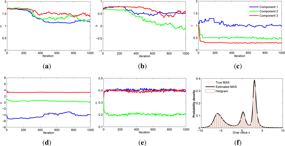
2.3. PSA Estimator for MAS Distributions

The Bayesian approach is an efficient technique for the estimation of MAS distribution parameters. This technique has received a lot of attention recently thanks to the evolution of MCMC computational tools. We name this the PSA estimator.
When estimating its parameters, it is convenient to consider the mixture model as a missing data problem. We assume that the data vector X = (x1, … , xj, … , xM) has been randomly drawn from K subpopulations. For each variable xj, let zj be an allocation variable for the unobserved or missing variable that indicates to which component xj belongs. Thus, zj will be equal to 1 if xj belongs to the kth subpopulation, or 0 otherwise.
Each observation xj is considered to be drawn from the kth component described by θk = (αk, βk, γk, μk) with probability
p ( z j = k | x j ) = ω k S α k ( x j | γ k , β k , μ k ) m = 1 K ω m S α m ( x j | γ m , β m , μ m )
The allocation variable zj can be defined as follows
z j = arg max k p ( k | x j )
Parameters then can be updated based on {zj}. The candidate parameter θ k new = ( α k new , β k new , γ k new , μ k new ) is sampled from a proposal distribution q(·|·), and is accepted with probability A θ k new, where
A θ k new = min ( 1 , ( j = 1 z j = k M S α k new ( x j | γ k new , β k new , μ k new ) S α k old ( x j | γ k old , β k old , μ k old ) ) 1 T ( t ) × p ( θ k new ) q ( θ k old | θ k new ) p ( θ k old ) q ( θ k new | θ k old ) )
In Equation (7), T(t) is the temperature function, which cools as the iteration proceeds. The introduction of T(t) can prevent the chain from trapping in small area, especially in case the target distribution may have multiple peaks. p(θ) is the prior function for parameter vector θ. In the case of an independent prior for each parameter, p(θ) can be expressed in terms of product p(θ) = p(α)p(β)p(γ)p(μ). We take the prior distributions of α, β, γ and μ to be uniform, uniform, inverse gamma (IG(·|·)) and normal (N(·|·)), respectively. In addition, we use a symmetric proposal satisfying q ( θ k new | θ k old ) = q ( θ k old | θ k new ) for simplicity. The acceptance probability A θ k new can then be simplified as
A θ k new = min ( 1 , ( j = 1 z j = k M S α k new ( x j | γ k new , β k new , μ k new ) S α k old ( x j | γ k old , β k old , μ k old ) ) 1 T ( t ) × I G ( γ k new | a 0 , b 0 ) N ( μ k new | ξ , κ ) I G ( γ k old | a 0 , b 0 ) N ( μ k old | ξ , κ ) )
where a0 and b0 are parameters of the inverse gamma prior for γ, and κ and ξ are parameters of the normal prior for μ. Moreover, a normal proposal distribution q(·|·) = N(·|δ, σ) is utilized in our algorithm, and its parameters are adaptively updated using estimations obtained in previous iterations: δ is set to the estimation of the previous iteration, and σ is set to the standard deviation of the previous L estimations. Adaptively updating the parameters of the proposal distribution ensures that new candidates can properly explore the entire parameter space, which further ensures that estimations rapidly converge to the true values.
The PSA estimator is described in Algorithm 1. The input includes observation X = (x1, x2, … , xM), the maximum iteration number Iter, the number of components K, starting temperature T(0), the value of L for updating the parameters of the proposal distribution, and the initial parameters θ k 0, ω k 0 for each component.
Algorithm 1. PSA estimator for parameters of MAS distributions
1:Input:
X = {xj}, θ k 0 = ( α k 0 , β k 0 , γ k 0 , μ k 0 ), ω k 0, k = 1, 2, … , K, L, T(0), Iter
2:for each t < Iter do
3:  Decrease temperature T ( t ) = T ( 0 ) lg ( t + 1 )
4:  Assign initial parameters θ k old = θ k t 1, ω k old = ω k t 1, k = 1, 2, … , K
5:  For each data sample xj, obtain allocation variable zj using Equation (6)
6:  Update parameters of the proposal distribution q(·|·) = N (·|δ, σ): set δ to value of the previous iteration and set σ to the standard deviation of the previous L estimations if t > L, otherwise set σ to its initialization value
7:  Sample new candidates θ k new = ( α k new , β k new , γ k new , μ k new ) from proposal distribution q|·) = N (·|δ, σ) for each component
8:  Accept θ k new according to Equation (8) and set θ k t = θ k new, otherwise set θ k t = θ k t 1
9:  Obtain weight ω = (ω1, … , ωk, …, ωK) of each component as in [27] by drawing samples from distribution ωD, where D(ζ + n1, …, ζ + nk, … ,ζ + nK) is the Dirichlet distribution with ζ > 0, and nk is the number of samples assigned to the kth component
10:end for
11:Output:
θk = (αk, βk, γk, μk), ωk, k = 1, 2, …, K
The critical differences between PSA estimator and Salas-Gonzalez’s method [27] are twofold. Firstly, PSA takes a cooling schedule, introducing T ( t ) = T ( 0 ) lg ( t + 1 ) over the acceptance probability. This ensures a reasonable probability of a downhill move, thus preventing the estimation from being trapped in small region of the parameter space for long periods of time. When the chain is trapped in small region, it is worthless to the estimation but will slow down the global convergence of the estimation. Secondly, in PSA estimator, parameters of the proposal distribution are adaptively updated by using the former estimations, which makes the proposal distribution increasingly closer to the distribution of the true parameter as the estimation procedure proceeds.

2.4. Simulation Result for PSA Estimator on MAS Distributions

To illustrate the effectiveness of the PSA estimator, we conduct an experiment using the MAS model shown in Equation (9). Random samples are generated using the algorithm proposed in [37].
p ( x ) = ω 1 S α 1 ( x | γ 1 , β 1 , μ 1 ) + ω 2 S α 2 ( x | γ 2 , β 2 , μ 2 ) + ω 3 S α 3 ( x | γ 3 , β 3 , μ 3 ) = 0.4 S 1.2 ( x | 1.0 , 0.5 , 4.25 ) + 0.2 S 1.2 ( x | 0.5 , 0.0 , 0.3 ) + 0.4 S 1.5 ( x | 0.3 , 0.5 , 3.25 )
As stated in Section 2.3, the priors are uniform for α and β, inverse Gamma for γ, and normal for μ. Initial values of the MAS distribution parameters are empirically chosen as follows: α1∼3 = [1.7, 1.7, 1.7], β1∼3 = [0.7, 0.7, 0.7], γ1∼3 = [1.0, 1.0, 1.0], μ1∼3 = [−4.0, 1.0, 4.0]. The parameters of inverse gamma prior for γ are a0 = 2 and b0 = 3, and those for the normal prior for μ are ξ = 0 and κ = 6. T(0) and L are set to 15 and 200, respectively. Experimental results for the PSA estimation with Iter = 1000 iterations are displayed in Figure 2(a–e). These show that the PSA estimator has a good convergence procedure. Figure 2(f) displays the discrete histogram of the originally simulated data, the PDF curve of the estimated MAS distributions with three components and the PDF curve of the true MAS distributions. This illustrates that the estimated MAS distributions fit the simulated data well.
To quantitatively evaluate the performance of the PSA estimator, we list in Table 1 true values, starting values, estimated values, and standard deviation (std) by PSA estimator. Results of Salas-Gonzalez’s method [27] are also included for comparison. Details of the initial conditions and implementation for Salas-Gonzalez’s method were reported in his work [27].
Table 1 shows that 9 of the 15 values estimated by PSA are closer to true values than the estimates given by Salas-Gonzalez’s method. The estimations of the two methods for ω1, ω2, ω3 and γ3 are similar and the estimations of PSA for two other parameters μ1 and μ3 are slightly worse than those of Salas-Gonzalez’s method. In addition, the standard deviation obtained by the proposed estimator is smaller than those of Salas-Gonzalez’s method. These results demonstrate the effectiveness of the proposed PSA estimator. Therefore, it can be concluded that the proposed PSA estimator is accurate for MAS distributions.

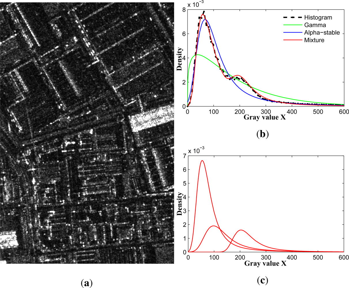
3. MAS-Based Statistical Modeling of SAR Images

A statistical model offers a description of SAR images’ statistical properties. The quality of classification depends on how well the statistical model agrees with the statistical properties. As mentioned in Section 1, many different models for SAR images exist, but these do not provide a good fit. The high probability of high intensities, produced by a large number of strong reflectors, leads to a heavy tail with a rather slow discrepancy in the SAR image histogram. In addition, each class of SAR image, especially at high resolutions, is usually a combination of different objects. For example, building areas generally contain strong reflectors, textures, and shadows. Such images present multimodal statistical properties; therefore, we expect that a multimodal distribution will be required to describe them.
We first analyze the performance of existing statistical models using TerraSAR-X image samples representing four different classes (river, marsh, farmland, and buildings). Each class contains 600 samples of 64 pixels × 64 pixels. Figure 3 displays eight samples from each class.
Kolmogorov–Smirnov (KS) test is applied to evaluate whether a particular model is able to describe the statistical properties of the SAR images. We calculate the KS distance (KSD) between the empirical distribution function (EDF) and the cumulative distribution function (CDF) of the reference distribution. The KSD is defined by Equation (10):
K S D = max n | F ( x n ) F ^ ( x n ) |
where F(xn) is the CDF and (xn) is the EDF. In addition, we also considered the acceptance probability, which is defined as the ratio of the number of samples that the KS test accepts for a distribution (at the 5% significance level) to the total number of samples in a class. The evaluation results are shown in Tables 2 and 3.
Table 2 shows that some models may be suitable for one class but not for another. Gamma distributions are not good for modeling marsh areas and building areas, because the corresponding average KSDs are particularly large. The Weibull and K distributions do not fit marsh areas well, whereas the G0 distribution can model marsh and building, but not river or farmland. This indicates that G0 distribution is suitable for modeling heterogeneous but not for homogeneous images. The Alpha-stable distribution is robust for various SAR image classes, as its average KSDs are not larger than 0.046, and it provides the best model for marsh areas. In addition, the maximum KSDs of the Alpha-stable distribution are the smallest of the different distributions tested. However, the average KSDs of the Alpha-stable distribution are still large. Similar results are also displayed in Table 3, which shows that Gamma distribution and Weibull distribution have a high probability of acceptance for modeling river and farmland, whereas they are always rejected for modeling the other two classes. The K distribution is always rejected when modeling marsh areas. The Alpha-stable distribution has a high probability of acceptance, but is not always accepted for modeling all four classes. These results indicate that unimodal distributions are not sufficient for modeling high-resolution SAR images due to the multimodal statistical properties inherent in such images.
To intuitively illustrate the multimodal statistical property of SAR image, we consider a 512 pixels × 768 pixels image of a building area from TerraSAR-X data. Figure 4 displays the original SAR image (Figure 4(a)), the fitting results (Figure 4(b)) of different models (including Gamma, Alpha-stable and MAS), and the estimated MAS distributions with three components (Figure 4(c)). From Figure 4(a), we can observe that many bright regions exist, caused by the existence of many strong reflectors in building area. Shadows of darkness are also observed, a result of the imaging mechanism of the SAR system, and few scatter waves are received by the SAR system in this kind of area. These factors lead to the complicated multimodal statistics of SAR images. In this case, none of unimodal distributions has the ability to model it well. Therefore, a multimodal distribution is necessary for accurate modeling of SAR images. MAS distributions can capture this essential statistical property pretty well.
We further evaluate the performance of MAS distributions with different number of components for modeling SAR image samples used previously. The results are shown in Tables 4 and 5.
From Tables 4 and 5, it can be concluded that MAS distributions substantially improve the modeling performances for all four classes. As we increase the number of components, the average KSD decreases and the acceptance probability increases for each class. The results also indicate that MAS distributions with five components are sufficient, as the average KSD and acceptance probability for each class change only slightly when the number of components increase to seven. Therefore, we choose the MAS distributions with five components to model the statistics of SAR images in the proposed classification algorithm.

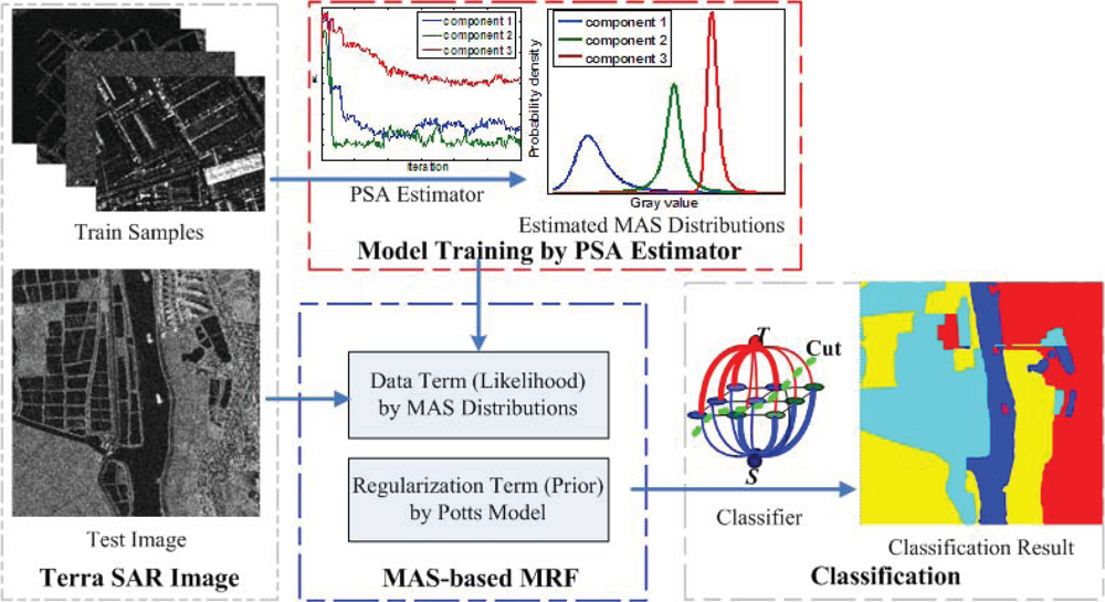
4. MAS-Based MRF Classification Algorithm

We propose the use of MAS distributions in a Bayesian classification scheme. MAS distributions are utilized to model the statistical properties of SAR images, and the spatial context is introduced by an MRF framework. A Graph Cuts-based algorithm is applied to obtain a global optimization.

4.1. MRF-Based Segmentation

Let X = (x1, … , xj, … , xM) be a random observation and Y = (y1, … , yj, … , yM) be the expected labeling result, with yj ∈ {1, 2, … , K}. In the Bayesian estimation framework, the SAR image classification could be described as a MAP problem, Ŷ = arg maxY P(Y|X). Based on the Bayesian theory, P(Y|X) ∝ P(X|Y)P(Y), it is equivalent with Ŷ = arg maxY P(X|Y)P(Y). The restoration method proposed in [38] assumes that the conditional probability of labeling Y = y, given an observation X = x, can be modeled by a Markov random field. Using the Hammersley–Clifford theorem, this probability can be written under Gibbs field formalism as Equation (11):
P ( Y = y | X = x ) = exp { U ( y | x ) } Z
where Z is a normalization coeffient, and U is the energy function given by the sum of a data term and a regularization term Equation (12):
U ( y | x ) = i ln p ( x j | y j ) + c C y V c ( y )
where Cy is the set of cliques of the selected neighborhood, and Vc is the potential of label configuration. In this paper, we focus solely on the data term, which is evaluated by mixture of Alpha-stable distributions. The second term is simply modeled by the Potts model [39], which can be written as Equation (13):
V C y = ( s , t ) ( y s , y t ) = { λ , y s y t λ , y s = y t
with s and t being in the same clique. Result of the Markovian segmentation is the label field Y = y that minimizes U (or equivalently maximizes P). In the energy function U of random field, mixture of Alpha-stable distributions are exploited to drive the data term.

4.2. MAS-Based MRF Classification Algorithm

We propose a supervised Bayesian classification algorithm by combining MAS distributions with MRF. Samples are required for each class to estimate the MAS distribution parameters via the PSA estimator. The first term of Equation (12) implies that the conditional probabilities are then represented by the MAS distributions. The regularization term is introduced via MRF, which builds a labeling restraint between the current pixel and its neighborhood. The classification turns out to be a posterior probability maximization problem, which is equivalent to minimizing the energy. To solve the energy minimization problem, we utilize a Graph Cuts optimization, as this is fast and obtains near-global optimization. The proposed MAS-based MRF classification algorithm is described in Figure 5.

5. Experiment and Result Analysis

The MAS-based MRF classifier was applied to the TerraSAR-X data. We compared the results from the MAS-based MRF classifier (MAS + MRF) with three other classifiers: Alpha-stable (AS)-based MRF classifier (AS + MRF), Gamma (GAM)-based MRF classifier (GAM + MRF), and mixture Gamma (MGAM)-based MRF classifier (MGAM + MRF). To enable a quantitative analysis, the classification accuracy for each class was calculated as the ratio of the number of correctly classified pixels to the total number of pixels in the class, given as a percentage with reference to the visually interpreted map. The regularity parameter for the Graph Cuts algorithm was empirically set to λ = 8.

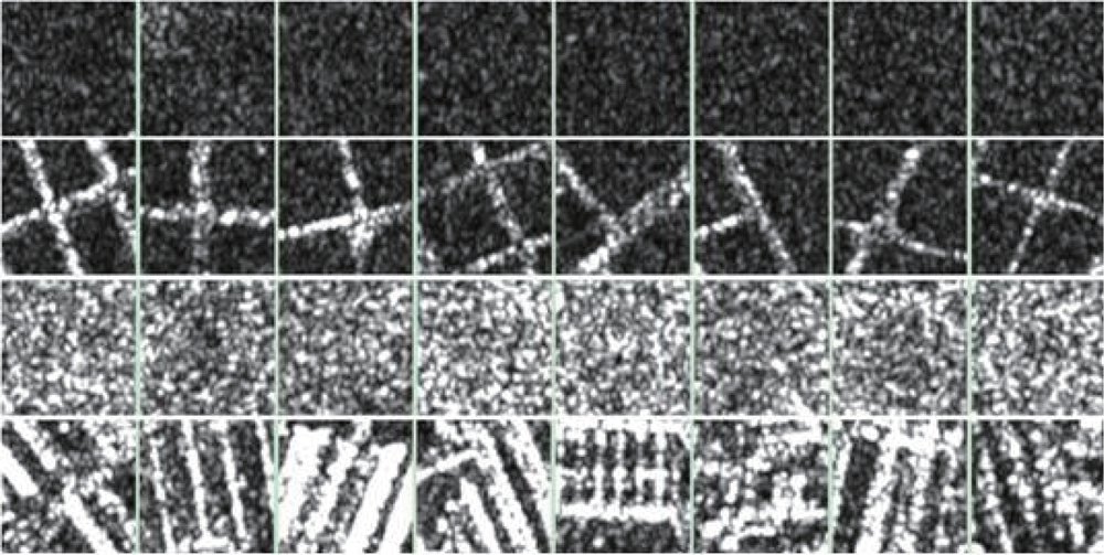
5.1. Experimental Data
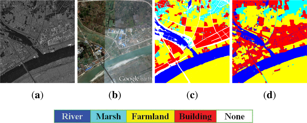
5.1.1. Wuhan Data

The TerraSAR-X data for Wuhan in Hubei, China, was acquired on 28 September 2008, with a spatial resolution of approximately 3.0 meters in range and azimuth (Stripmap mode, multilook ground range detected). The image, shown in Figure 6(a), has a size of 2,000 pixels × 1,800 pixels. Figure 6(b) is the optical image from Google Earth (© Google 2013). Figure 6(c) is the visually interpreted map. A total of four land covers were identified, namely river, marsh, farmland, and buildings. The white areas labeled ‘None’ in Figure 6(c) could not be defined. These regions were not included in the accuracy assessment step.

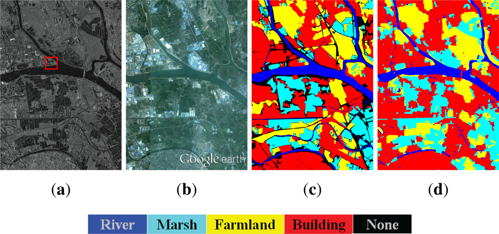
5.1.2. Foshan Dataset

The TerraSAR-X data for Foshan in Guangdong, China, was acquired on 24 May 2008, with a spatial resolution of approximately 1.25 meters in both range and azimuth (Stripmap mode, multilook ground range detected). The image, shown in Figure 7(a), has a size of 7,000 pixels × 5,000 pixels. Figure 7(b) is the optical image from Google Earth (© Google 2013). Figure 7(c) is the visually interpreted map. Again, four land covers were identified, i.e., river, marsh, farmland, and buildings. The black areas labeled ‘None’ in Figure 7(c) could not be defined. These regions were not included in the accuracy assessment step.

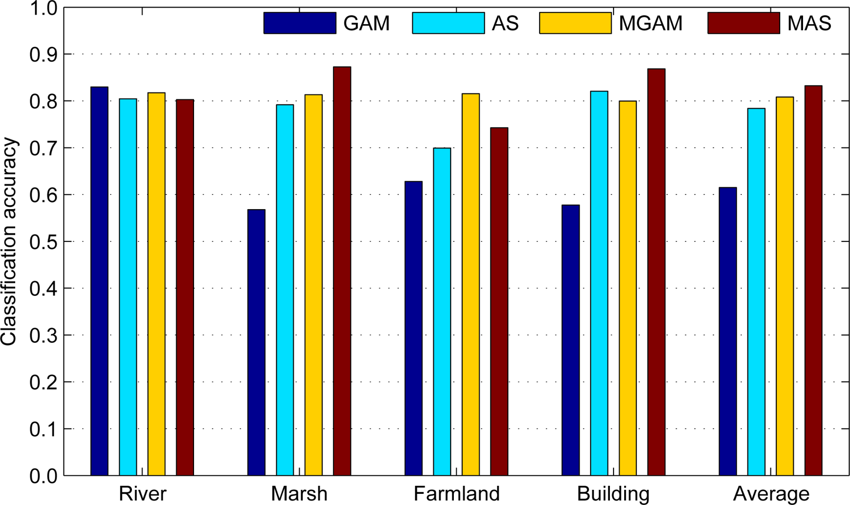
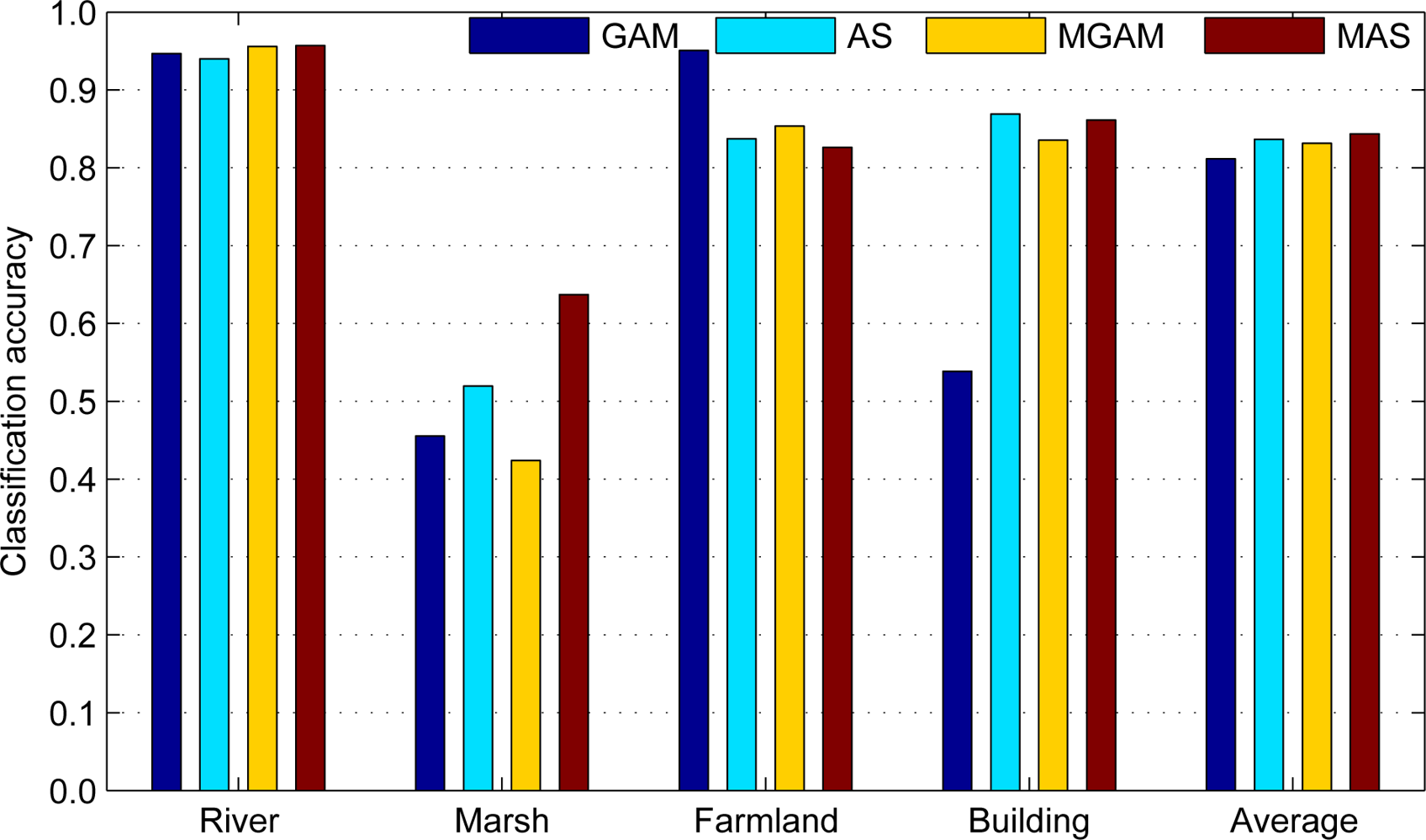
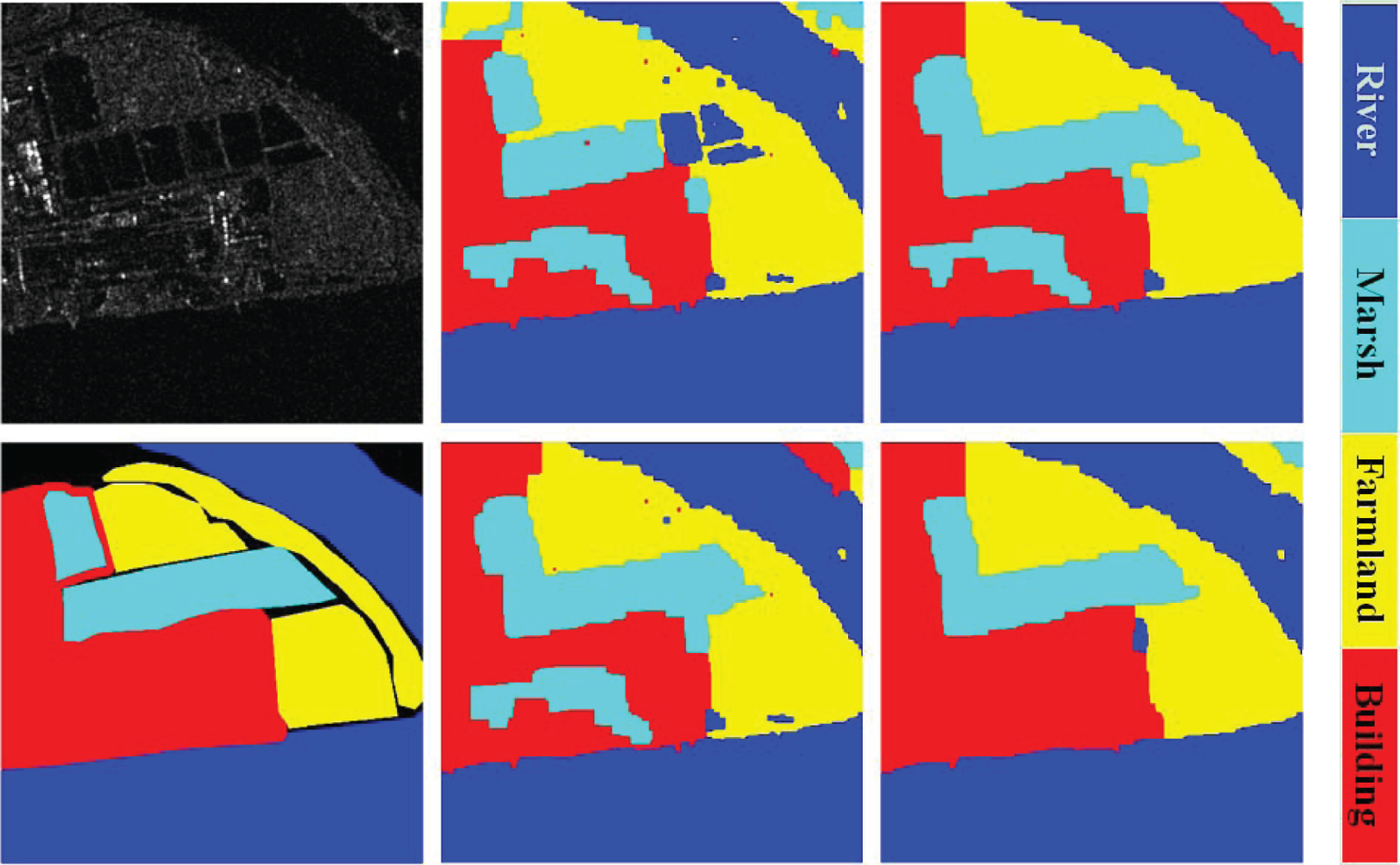
5.2. Classification Result

In this experiment, samples were selected from each class in order to learn the parameters of the MAS distributions. The Potts model was applied to introduce the spatial contextual information, which behaves as the regularization term. Various classifiers were selected to compare their classification performance. The results from the MAS + MRF classifier for the Wuhan and Foshan data are displayed in Figures 6(d) and 7(d), respectively. These both show that the global ground cover acquired by the MAS + MRF classifier was well recognized. In particular, the region edges were accurate. In our experiment, we found that the AS + MRF classifier and the MGAM + MRF classifier also obtained acceptable classification results, but those of the GAM + MRF classifier were poor, especially for marsh areas, which were probably mislabeled as rivers.

5.3. Result Analysis

The classification accuracy for each class, as well as the average accuracy, was calculated for different classifiers. Confusion matrices for the results obtained by the MAS+MRF classifier on Wuhan data and Foshan data are displayed in Tables 6 and 7. In addition, the classification accuracy for each class and the overall accuracy of different classifiers are illustrated in Figures 8 and 9.
Tables 6 and 7 show that the MAS + MRF classifier obtains a high accuracy for each class on both Wuhan data and Foshan data, with an average accuracy of 84.35% and 83.22%, respectively.
Figure 8 illustrates that the MAS + MRF classifier attains an average accuracy of 84.35% for the Wuhan data, which is higher than that of the other classifiers by 0.69%–3.21%. The average accuracies are 83.12%, 83.66% and 81.14% for MGAM + MRF, AS + MRF and GAM + MRF, respectively. Similarly, Figure 9 shows that the MAS+MRF classifier is the most accurate for marsh and building with the Foshan data, and obtains good results for river and farmland. The average accuracy obtained by MAS + MRF is higher than that of the other classifiers by 2.41%–21.74%. The average accuracies are 61.48%, 78.40%, 80.81% and 83.22% for GAM + MRF, AS + MRF and MGAM + MRF, respectively. This leads us to the conclusion that the MAS + MRF classifier outperforms the other classifiers. In addition, it can also be concluded that a classifier based on a mixture of distributions obtains better classification accuracy than a single distribution classifier. The improvement given by the mixture model is obvious. The high accuracy of classification by the MAS-based MRF classifier can be explained by the accurate modeling of the multimodal statistical properties of SAR images.
To evaluate the performance of the various classifiers in a localized area, we studied the 480 pixels × 480 pixels image indicated by the red box in Figure 7(a). The visually interpreted map and classifications are displayed in Figure 10. The GAM + MRF classifier result is not good, as it misclassifies large areas of marsh as river. The AS + MRF classifier and MGAM + MRF classifier obtain slightly better classification results than GAM + MRF. However, all three classifiers misclassify large areas of buildings as marsh. Fortunately, the proposed MAS + MRF classifier correctly labels these areas. It can be observed that different regions are perfectly distinguished, and the edges are also accurate. These results further illustrate the efficiency of the proposed MAS + MRF classifier.

6. Conclusions

This paper proposed the mixture of Alpha-stable distributions, the first application in image processing, to model the multimodal and impulsive statistical properties of SAR images especially at high resolution, and introduced a PSA estimator to determine the distribution parameters. Simulation results on simulated data validated the effectiveness of the PSA estimator, and the modeling performance over TerraSAR-X samples verified the validity of MAS distributions for SAR images. Finally, a Bayesian classification algorithm that combines MAS distributions and MRF was presented for SAR images. The classification performances over TerraSAR-X images demonstrated that the proposed mixture model is a promising candidate for the modeling and classification of SAR images and can be potentially useful for SAR images analysis, interpretation, and other important applications.

Acknowledgments

This work was supported in part by the National Basic Research Program of China (973) (No. 2011CB707102), in part by the National Natural Science Foundation of China (No. 40871199), and in part by the Fundamental Research Funds for the Central Universities (No. 20102120201000128).
The authors would like to thank the editor and all the reviewers for their helpful suggestions and comments on this paper.
  • Conflict of InterestThe authors declare no conflict of interest.

References

  1. Perko, R.; Raggam, H.; Deutscher, J.; Gutjahr, K.; Schardt, M. Forest assessment using high resolution SAR data in X-band. Remote Sens. 2011, 3, 792–815. [Google Scholar]
  2. Alberga, V. Similarity measures of remotely sensed multi-sensor images for change detection applications. Remote Sens. 2009, 1, 122–143. [Google Scholar]
  3. Hasager, C.B.; Badger, M.; Pena, A.; Larsén, X.G.; Bingol, F. SAR-based wind resource statistics ′ in the Baltic Sea. Remote Sens. 2011, 3, 117–144. [Google Scholar]
  4. Tison, C.; Nicolas, J.M.; Tupin, F.; Maitre, H. A new statistical model for Markovian classification of urban areas in high-resolution SAR images. IEEE Trans. Geosci. Remote Sens. 2004, 42, 2046–2057. [Google Scholar]
  5. Jacob, A.M.; Hemmerly, E.M.; Fernandes, D. SAR Image Classification Using a Neural Classifier Based on Fisher Criterion. In Proceedings of the 7th Brasilian Symposium on Neural Networks (SBRN02), Recife, Brazil, 11–14 November 2002; pp. 168–172.
  6. Chamundeeswari, V.V.; Singh, D.; Singh, K. Unsupervised Land Cover Classification of SAR Images by Contour Tracing. In Proceedings of Geoscience and Remote Sensing Symposium (IGARSS 2007), Barcelona, Spain, 23–27 July 2007; pp. 547–550.
  7. Oliver, C.J. Understanding Synthetic Aperture Radar Images; Artech House: Boston, MA, USA/London, UK, 1998. [Google Scholar]
  8. Oliver, C. Optimum texture estimators for SAR clutter. J. Phys. D Appl.Phys. 1993, 26, 1824–1835. [Google Scholar]
  9. Menon, M. Estimation of the shape and scale parameters of the Weibull distribution. Technometrics 1963, 5, 175–182. [Google Scholar]
  10. Szajnowski, W. Estimators of log-normal distribution parameters. IEEE Trans. Aerosp Electron. Syst. 1977, AES-13, 533–536. [Google Scholar]
  11. Jakeman, E.; Pusey, P. A model for non-Rayleigh sea echo. IEEE Trans. Antennas Propagat. 1976, 24, 806–814. [Google Scholar]
  12. Jao, J.K. Amplitude distribution of composite terrain radar clutter and the K-distribution. IEEE Trans. Antennas Propag. 1984, AP-32, 1049–1062. [Google Scholar]
  13. Li, H.C.; Hong, W.; Wu, Y.R.; Fan, P.Z. On the empirical-statistical modeling of SAR images with generalized gamma distribution. IEEE J. Sel. Top. Signal Process. 2011, 5, 386–397. [Google Scholar]
  14. Galland, F.; Nicolas, J.M.; Sportouche, H.; Roche, M.; Tupin, F.; Refregier, P. Unsupervised synthetic aperture radar image segmentation using fisher distributions. IEEE Trans. Geosci. Remote Sens. 2009, 47, 2966–2972. [Google Scholar]
  15. Frery, A.; Muller, H.-J.; Yanasse, C.; Sant’Anna, S. A model for extremely heterogeneous clutter. IEEE Trans. Geosci. Remote Sens. 1997, 35, 648–659. [Google Scholar]
  16. Kuruoglu, E.E.; Zerubia, J. Modeling SAR images with a generalization of the Rayleigh distribution. IEEE Trans. Image Process. 2004, 13, 527–533. [Google Scholar]
  17. Achim, A.; Tsakalides, P.; Bezerianos, A. SAR image denoising via bayesian wavelet shrinkage based on heavy-tailed modeling. IEEE Trans. Geosci. Remote Sens. 2003, 41, 1773–1784. [Google Scholar]
  18. Gao, G.; Shi, G.T.; Zou, H.X.; Zhou, S.L. Characterizing the statistical properties of SAR clutter by using an empirical distribution. Int. J. Antennas Propag. 2013, 109145:1–109145:8. [Google Scholar] [CrossRef]
  19. Gao, G. Statistical modeling of SAR images: A survey. Sensors 2010, 10, 775–795. [Google Scholar]
  20. Liao, M.S.; Wang, C.C.; Wang, Y.; Jiang, L.M. Using SAR images to detect ships from sea clutter. IEEE Geosci. Remote Sens. Lett. 2008, 5, 194–198. [Google Scholar]
  21. Chen, J.Y.; Sun, H. Multi-Resolution Edge Detection Based on Alpha-Stable Model in SAR Images Using Translation-Invariance Contourlet Transform. In Proceedings of Signal Processing and Information Technology (ISSPIT 2006), Vancouver, BC, Canada, 27–30 August 2006; pp. 264–270.
  22. Peng, Y.J.; Xu, X.; Zhou, W.B.; Zhao, Y. SAR image classification based on alpha-stable distribution. Remote Sens. Lett. 2011, 2, 51–59. [Google Scholar]
  23. Wan, T.; Canagarajah, N.; Achim, A. Segmentation-driven image fusion based on alpha-stable modeling of wavelet coefficients. IEEE Trans. Multimed. 2009, 11, 624–633. [Google Scholar]
  24. Deng, C.Z.; Zhu, H.S.; Wang, S.Q. Curvelet Domain Watermark Detection Using Alpha-Stable Models. In Proceedings of Information Assurance and Security (ICIAS 2009), XI’an, China, 18–20 August 2009; pp. 313–316.
  25. Ge, X.H.; Zhu, G.X.; Zhu, Y.T. On the testing for alpha-stable distributions of network traffic. Comput. Commun. 2004, 5, 447–457. [Google Scholar]
  26. Xu, W.D.; Wu, C.F.; Dong, Y.C. Modeling Chinese stock returns with stable distribution. Math. Comput. Modell. 2011, 54, 610–617. [Google Scholar]
  27. Salas-Gonzalez, D.; Kuruoglu, E.E.; Ruiz, D.P. Finite mixture of alpha-stable distributions. Digital Signal Process. 2009, 19, 250–264. [Google Scholar]
  28. Salas-Gonzalez, D.; Kuruoglu, E.E.; Ruiz, D.P. Modelling with mixture of symmetric stable distributions using Gibbs sampling. Signal Process. 2009, 90, 774–783. [Google Scholar]
  29. Salas-Gonzalez, D.; Kuruoglu, E.E.; Ruiz, D.P. Bayesian Estimation of Mixtures of Skewed Alpha-Stable Distributions with an Unknown Number of Components. In Proceedings of European Signal Processing, EUSIPCO 2006, Florence, Italy, 4–8 September 2006.
  30. Buckle, D.J. Bayesian inference for stable distribution. J. Am. Stat. Assoc. 1995, 90, 605–613. [Google Scholar]
  31. Casarin, R. Bayesian Inference for Mixtures of Stable Distributions; Working Paper No. 0428; CEREMADE, University Paris IX: Paris, France, 2004. [Google Scholar]
  32. Boykov, Y.; Veksler, O.; Zabih, R. Fast approximate energy minimization via Graph Cuts. IEEE Trans. Pattern Anal. Mach. Intell. 2001, 23, 1222–1239. [Google Scholar]
  33. Kolmogorov, V.; Zabih, R. What energy functions can be minimized via Graph Cuts? IEEE Trans. Pattern Anal. Mach. Intell 2004, 26, 147–159. [Google Scholar]
  34. Boykov, Y.; Kolmogorov, V. An experimental comparison of Min-Cut/Max-Flow algorithms for energy minimization in vision. IEEE Trans. Pattern Anal. Mach. Intell. 2004, 26, 1124–1137. [Google Scholar]
  35. Levy, P. Theorie des erreurs : La loi de Gauss et les lois exceptionnelles. Bull. Socit Mathmatique France 1924, 52, 49–85. [Google Scholar]
  36. Belov, I.A. On the Computation of the Probability Density Function of Alpha-Stable Distributions. In Proceedings of the 10th International Conference on Mathematical Modelling and Analysis (ICMMA 2005), Trakai, Lithuania, 1–5 June 2005; pp. 333–341.
  37. Chambers, J.; Mallows, C.; Stuck, B. A method for simulating stable random variables. J. Am. Stat. Assoc. 1976, 71, 340–344. [Google Scholar]
  38. Geman, S.; Geman, D. Stochastic relaxation, Gibbs distribution, and the Bayesian restauration of images. IEEE Trans. Pattern Anal. Mach. Intell. 1984, PAMI-6, 721–741. [Google Scholar]
  39. Wu, F. The Potts model. Rev. Mod. Phys. 1982, 54, 235–268. [Google Scholar]
Figure 1. PDF of Alpha-stable distributions (μ = 0). (a) Symmetric Alpha-stable case: α = [0.4,0.7,1.0,1.3,2.0], β = 0.0, γ = 1.0; (b) Enlargement of the tails in (a); (c) Skewness parameter: α = 1.2, β = [0.0,0.2,0.5,0.8,1.0], γ = 1.0; (d) Dispersion parameter: α = 1.6, β = 0.0, γ = [0.3,0.6,1.0,2.0,3.0].
Remotesensing 05 02145f1
Figure 2. Simulation results for the PSA estimator. (a)–(e) Evolution procedure of the three components for parameters α, β, γ, μ and ω, respectively (red: component 1, green: component 2, blue: component 3); (f) Fitting results of the estimated MAS distributions to simulated data histogram and the PDF curve obtained by the true parameters.
Remotesensing 05 02145f2
Figure 3. Eight samples from each class (from top to bottom: river, marsh, farmland and building).
Remotesensing 05 02145f3
Figure 4. Selected building area and fitting results. (a) Building area in SAR image; (b) Fitting results by different models; (c) Three components of the estimated MAS distributions.
Remotesensing 05 02145f4
Figure 5. Flowchart of the MAS-based MRF classification algorithm.
Remotesensing 05 02145f5
Figure 6. TerraSAR-X data of Wuhan city. (a) SAR image of Wuhan, Hubei, China; (b) Optical image from Google Earth (© Google 2013); (c) Visually interpreted map; (d) Classification result of MAS + MRF classifier.
Remotesensing 05 02145f6
Figure 7. TerraSAR-X data of Foshan city. (a) SAR image of Foshan, Guangdong, China; (b) Optical image from Google Earth (© Google 2013); (c) Visually interpreted map; (d) Classification result of MAS + MRF classifier.
Remotesensing 05 02145f7
Figure 8. Classification accuracies of different classifiers on Wuhan dataset.
Remotesensing 05 02145f8
Figure 9. Classification accuracies of different classifiers on Foshan dataset.
Remotesensing 05 02145f9
Figure 10. Classifications of localized area (top, left–right: SAR image, result from GAM + MRF, result from AS + MRF; bottom, left–right: Visually interpreted map, result from MGAM + MRF, result from MAS + MRF).
Remotesensing 05 02145f10
Table 1. Simulation results for the PSA estimator on MAS distributions.
ParameterPSASalas-Gonzalez

NameTrueStartingEstimatedstdEstimatedstd
α11.201.701.200.021.270.09
β10.500.700.530.010.650.08
γ11.001.001.010.020.980.06
μ1−4.25−4.00−4.110.19−4.300.60
ω10.400.330.400.010.400.02

α21.201.701.280.071.300.17
β20.000.70−0.030.070.040.30
γ20.501.000.470.020.450.05
μ20.301.000.250.070.400.30
ω20.200.330.200.010.200.02

α31.501.701.450.041.370.12
β30.500.700.510.080.340.20
γ30.301.000.300.010.300.02
μ33.254.003.280.023.240.06
ω30.400.330.400.010.400.02
Table 2. Kolmogorov–Smirnov distance (KSD) of different statistical models.
Average KSD (Maximum KSD)

ModelRiverMarshFarmlandBuilding
Gamma0.042 (0.213)0.205 (0.427)0.044 (0.172)0.280 (0.590)
Weibull0.058 (0.207)0.109 (0.171)0.047 (0.164)0.085 (0.152)
G00.118 (0.915)0.051 (0.100)0.145 (0.806)0.035 (0.287)
K0.024 (0.133)0.081 (0.164)0.014 (0.069)0.064 (0.287)
Alpha-stable0.046 (0.079)0.027 (0.071)0.042 (0.072)0.039 (0.100)
Table 3. Acceptance probability of different statistical models.
Acceptance Probability at 5% Significance Level (Percentage)

ModelRiverMarshFarmlandBuilding
Gamma81.170.1771.670.00
Weibull55.330.0070.330.67
G083.8345.4481.6983.33
K97.004.1799.8343.83
Alpha-stable68.8396.5070.8367.50
Table 4. Mixture of Alpha-stable distributions for modeling various SAR images.
Average KSD (Maximum KSD)

ComponentsRiverMarshFarmlandBuilding
10.046 (0.079)0.027 (0.071)0.042 (0.072)0.039 (0.100)
30.025 (0.050)0.024 (0.088)0.012 (0.049)0.026 (0.099)
50.021 (0.041)0.023 (0.113)0.011 (0.025)0.024 (0.115)
70.021 (0.074)0.022 (0.110)0.010 (0.023)0.023 (0.115)
Table 5. Acceptance probability of mixture models with different number of components.
Acceptance Probability at 5% Significance Level (Percentage)

ComponentsRiverMarshFarmlandBuilding
168.8396.5070.8367.50
399.8396.83100.0087.17
5100.0097.17100.0088.67
7100.0098.00100.0089.33
Table 6. Confusion matrix for the MAS + MRF result (percentage).
DatasetWuhan data (Average accuracy: 84.35)

ClassRiverMarshFarmlandBuilding
River95.70.71.22.4
Marsh22.263.72.511.6
Farmland0.61.382.615.5
Building3.60.79.686.1
Table 7. Confusion matrix for the MAS + MRF result (percentage).
DatasetFoshan data (Average accuracy: 83.22)

ClassRiverMarshFarmlandBuilding
River80.311.22.06.5
Marsh4.087.33.45.3
Farmland0.30.974.324.5
Building0.710.02.586.8

