Compact Multipurpose Mobile Laser Scanning System — Initial Tests and Results


Abstract
: We describe a prototype compact mobile laser scanning system that may be operated from a backpack or unmanned aerial vehicle. The system is small, self-contained, relatively inexpensive, and easy to deploy. A description of system components is presented, along with the initial calibration of the multi-sensor platform. The first field tests of the system, both in backpack mode and mounted on a helium balloon for real-world applications are presented. For both field tests, the acquired kinematic LiDAR data are compared with highly accurate static terrestrial laser scanning point clouds. These initial results show that the vertical accuracy of the point cloud for the prototype system is approximately 4 cm (1σ) in balloon mode, and 3 cm (1σ) in backpack mode while horizontal accuracy was approximately 17 cm (1σ) for the balloon tests. Results from selected study areas on the Sacramento River Delta and San Andreas Fault in California demonstrate system performance, deployment agility and flexibility, and potential for operational production of high density and highly accurate point cloud data. Cost and production rate trade-offs place this system in the niche between existing airborne and tripod mounted LiDAR systems.1. Introduction
Airborne LiDAR (Light Detection and Ranging) systems have become a standard mechanism for acquiring dense, high-precision topography, making it possible to perform large surveys (100’s of km2 per day) at spatial scales as fine as a few decimeters horizontally and a decimeter or better vertically [1–4]. Information collected by LiDAR technology has been applied to a wide variety of science and engineering applications including archaeological exploration, developing and managing natural resources, mitigating the impacts of such natural disasters as floods, hurricanes, storm surge, landslides and sinkholes, and building and maintaining transportation infrastructure [5–8]. In the Earth Sciences, the use of LiDAR datasets has also rapidly expanded. For example, over the past ten years high resolution LiDAR topography has played an important role in furthering the understanding and documentation of earthquakes and their effects along major plate boundary fault systems [9–12].
However, current airborne and terrestrial LiDAR systems suffer from a number of drawbacks. They are expensive, bulky, require significant power supplies, and are often optimized for use in only one type of platform. Often, particularly with airborne systems, it takes significant logistical efforts and planning to relocate the LiDAR instruments to project sites, especially when the study areas are in remote locations. This poses a significant challenge when precise topographic mapping is needed in response to natural events such as earthquakes and hurricanes for example. It would therefore be advantageous to have a lightweight, compact and relatively inexpensive multipurpose LiDAR and imagery system that could be used from a variety of moving platforms—both terrestrial and airborne. The system should be quick and easy to deploy, and require a minimum amount of existing infrastructure for operational support. These operational requirements also need to be balanced with the stringent accuracy requirements of our target science and engineering applications, which ideally require both high accuracy (vertical accuracy <10 cm, horizontal accuracy <20 cm (1σ)), and high point densities (preferably >10 pts/m2).
An initially analysis of the challenges posed above would suggest that perhaps a unmanned aerial vehicle (UAV) based laser scanning platform would be a suitable alternative. Over the past several years there have been a few successful data collections with LiDAR scanners mounted on UAV platforms [13–16]. All of these systems have taken advantage of lightweight IMU systems and laser scanners in order to limit the overall remote sensing payload. The light payload however comes with a sacrifice to the expected accuracy of the acquired point cloud. For example, [13–15] all take advantage of the Ibeo Lux scanner, which has only a 10 cm ranging accuracy, and a 14 mrad beam divergence [14], which can cause significant horizontal uncertainty in the resulting point cloud. In addition, all of the systems in [13–16] take advantage of low cost MEMs sensors, which have comparably high noise values and drift rates that significantly degrade the expected accuracy of their attitude solution. Therefore, to target our science and engineering applications, with their more stringent accuracy requirements, we required a remote sensing payload with improvements in the accuracy of both the laser scanner, and the IMU.
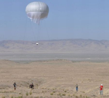
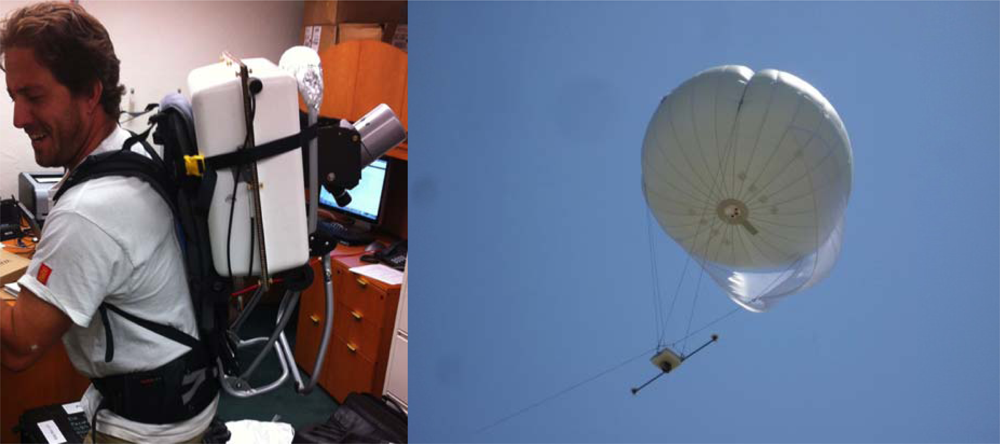
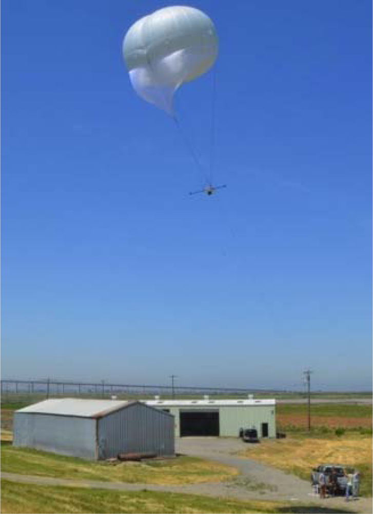
With the above goals in mind, we have developed a field deployable compact dynamic laser scanning system that is configured for use on a variety of platforms, including backpack mounts, unmanned aerial vehicles (e.g., balloons and helicopters) and small off-road vehicles such as ATV’s. The system is small (<15 kg), self-contained, relatively inexpensive (<$100K USD), and easy to deploy. The first version of this compact LiDAR system has been successfully tested in both backpack configuration and on a tethered flight attached to a helium balloon (see Figure 1). The remainder of this article discusses the prototype system, and initial te ting and analysis of the data collected with it. Section 2 gives a brief description of the components that make up the LiDAR system. Section 3 discusses the calibration and analysis of the combined system to ensure highly accurate georeferenced point clouds. Section 4 presents the initial tests of the system both in backpack and balloon deployments. Section 5 gives an initial analysis of the first datasets acquired with the system, and compares them to high accuracy terrestrial laser scanning (TLS). Finally, Sections 6 and 7 present our conclusions and planned future testing of the system and ideas for its further improvement and refinement.
2. System Description and Components
2.1. System Components
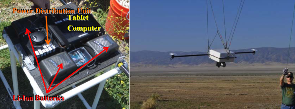
The current prototype sensor pod contains, a Velodyne HDL-32E LiDAR scanner which operates at a nominal pulse rate of 700 kHz, an Oxford Technical Solutions Inertial+2 INS (Inertial Navigation System), dual Novatel GNSS (Global Navigation Satellite System) receivers, a ruggedized tablet computer for system control and data logging, and redundant Li-Ion battery packages. Technical specifications of the Velodyne laser scanner and OxTS IMU are given in Tables 1 and 2, respectively.
The current system configuration (including cabling, packaging and power supply) has a mass of roughly 15 kg, and is capable of approximately 6 hour missions. Mission duration is limited by the available power in the current battery packs, and the amount of onboard hard drive capacity in the data logging computer. Images of the system taken during field testing are given in Figure 2. The image on the left shows the pod with the top cover removed, and reveals the Li-Ion batteries, along with the logging and control computer. The right image shows the laser scanner mounted on the balloon, and shows the laser sensor protruding from the bottom of the instrument pod. The laser scanner rotation axis is perpendicular to the flight direction. Note that a dual GPS receiver configuration is used for the system. Due to the low motion dynamics in both the backpack and balloon mounted mode the IMU attitude accuracy can drift significantly. Introducing a precise heading constraint to the IMU solution through the 4 m GPS baseline on the pod significantly improves the accuracy of the attitude estimation of the system during extended periods of low dynamics and allows the attitude accuracy to remain close to the manufacturer stated accuracies given in Table 2.
2.2. Data Acquisition and Post Processing
In order to produce the highest quality geodetic data from the multipurpose laser scanning system, it has been configured for all data processing tasks to be performed post-mission. Raw data from all sensors (GNSS, INS, laser scanner) are recorded by the logging and control computer on board the instrument package. After data acquisition, the raw GNSS observations from the onboard Novatel receivers (2 Hz data rate) are combined with raw measurements from GNSS base station(s) to determine a precise kinematic trajectory for the platform using the GrafNav software package. The GNSS trajectory is then blended with the 100 Hz raw inertial measurements in a loosely-coupled Kalman Filter using Oxford Technical Solutions RT-PostProcess software package, which results in an optimal estimate of platform position and attitude. Finally, the estimated platform trajectory and attitude (at 100 Hz) is combined with the raw range and angle measurements from the Velodyne laser sensor and the system calibration parameters (Sections 3.2 and 3.3), using software developed by the research team, to generate the final LiDAR point cloud. The software package applies the mathematical model for the Velodyne scanner observations (Equation (1)), and the LiDAR georeferencing formula (Equation (2)) that are presented and discussed in Section 3.
3. System Calibration and Validation
3.1. Georeferencing Mathmatical Model
The Velodyne HDL-32E scanner is composed of 32 individual laser-detector pairs which are individually aimed in 1.33° increments over the 40° field of view of the laser scanner. The calculation of of (x,y,z) coordinates in the scanners own coordinate system is identical to that of the Velodyne HDL-64E scanner given in [17], as:
si is the distance scale factor for laser i;
is the distance offset for laser i;
δi is the vertical rotation correction for laser i;
βi is the horizontal rotation correction for laser i;
is the horizontal offset from scanner frame origin for laser i;
is the vertical offset from scanner frame origin for laser i;
Ri is the raw distance measurement from laser i;
ε is the encoder angle measurement.
The first six parameters are interior instrument specific calibration values (interior calibration), and are supplied by the manufacturer in a xml document with each scanner. The final two values (Ri and ε) are the observations returned by the scanner assembly for each individual laser.
Given the coordinates of the object point in the scanner’s own coordinate system, it is then desirable to calculate the laser return locations in a global geodetic reference frame. Calculation of global coordinates for objects from laser scanning system observations has been well documented in prior literature [18–20]. Coordinates on the ground may be calculated by combining the information from the laser scanner, integrated GNSS/INS navigation system and calibration values including ground reference. The target coordinate equation is given as:
coordinates of LiDAR impingement point in global frame;
coordinates of navigation sensor center in global frame;
rotation matrix from navigation sensor body (b) frame local level frame, defined by the three rotation angles roll, pitch and yaw;
boresight calibration matrix: the rotation from laser scanner’s own coordinate system (s) frame into (b) frame;
rs coordinates of target point given in laser scanner’s own coordinate frame;
lb lever-arm from scanner to navigation center origin given in the body frame.
All of the above values are provided, either by the laser scanner itself (rs), or by the GPS/INS navigation system, except for the boresight calibration matrix, and the lever-arm offset vector, both of which must be determined by system calibration. The boresight calibration process to determine these values is described in greater detail in Section 3.3.
3.2. Static Laser Scanner Calibration
The Velodyne HDL-32E scanner is provided with an instrument manufacturer calibration, and sample source code that easily allows the user to derive local scanner coordinates for all observations from the laser-detector pairs of the sensor. This, in principle, gives the user the ability to determine local scanner coordinate point cloud files readily. In previous studies of an earlier model of Velodyne scanner, the HDL-64E S2, it was found, however, that the relative accuracy of the point cloud could be dramatically improved by performing a rigorous static calibration of the scanner in order to improve upon the Velodyne factory scanner calibration. This static calibration procedure is given in detail in [17,21]. This same procedure was undertaken for the Velodyne HDL-32E sensor. To evaluate if there was improvement in the relative accuracy of the resultant point cloud, 3D misclosure vectors with respect to known planar surfaces were calculated for approximately 100,000 points in the static calibration datasets, both before and after the adjustment of the laser system calibration parameters. Table 3 shows the relative 3D root mean square errors (3D RMSE) from the static calibration point cloud before and after interior calibration adjustment.
The results in Table 3 show an approximately 20% improvement in the relative accuracy of the point cloud obtained by the Velodyne HDL-32E with the supplemental interior orientation calibration. Given that we are trying to achieve as high accuracy as possible from our integrated system, a 20% improvement is fairly substantial. As a result, the improved interior calibration model was used for all of the subsequent data processing and analysis of the system.
3.3. Boresight and Lever-Arm Calibration
Additional calibration values are required to accurately transform the point cloud from the scanner’s own coordinate system into a global coordinate system. These calibration values are the boresight calibration matrix (angular offsets between INS and laser scanner axes), and the lever arm offset (positional offset between INS and laser scanner origins). In practice the boresight calibration matrix may only be determined by analysis of georeferenced point cloud data obtained from the laser scanning system. There are a variety of ways to determine these values, see for example [19,22,23]. For the developed system, the approach detailed in [23,24] was used to simultaneously estimate the boresight angles and the horizontal lever arm components using a non-linear least squares approach. The vertical component of the lever-arm is very weakly observable, and therefore is estimated using the engineering drawings of the subcomponents and overall system assembly.
The boresight methodology implemented requires a dataset containing numerous planar surfaces that have been collected by the LiDAR system from more than one viewing direction. To collect such a dataset, the instrument package was mounted on a balloon and tethered to a pickup truck that was then used to pull the balloon past a series of buildings in multiple directions (Figure 3) at a height of approximately 25 m above ground level. The LiDAR data returns from planar surfaces was then manually extracted and used in the least squares adjustment to determine the boresight values. Each extracted planar surface had a maximum size of 2 m by 2 m to minimize any possible distortions of the reference surfaces (e.g., due to bowed rooftops). The five estimated values and their estimated standard deviations with covariance propagation through the least squares solution are given in Table 4. The results show that the lever arm components were estimated with mm level accuracy, while the angular offsets were estimated with 1–2 milli-degree accuracy. These estimated accuracies are well below the expected noise level of the GNSS/INS navigation trajectory.
Because the planar surfaces used in the least squares adjustment have been observed by the system at multiple times and with differing view geometry we can state that, in the absence of systematic errors, the RMSE (root mean square error) of the planar misclosure residuals after the adjustment will give a good indication of the noise level of the combined mobile scanner/GNSS/INS system [24]. For the calibration adjustment there were 45 extracted planar surfaces with approximately 225,000 total laser return points. Statistical measures on the misclosure vectors are presented in Table 5. Note that for the computed values in Table 5 misclosure vectors larger than 5σ have been removed. These 5σ outliers represent less than 0.7% of the analyzed points.
Table 5 shows that the balloon mounted system has a 3D agreement from overlapping passes of approximately 9 cm for hard surface targets. This level of agreement is very close to the combined noise level of the LiDAR and navigation components of the system and suggests that there are no significant systematic error sources remaining in the calibrated point clouds.
It should be noted that the results above pertain to calibrating the system in balloon mode only. The calibration for backpack mode is carried out in a similar manner, only in this case the calibration dataset is obtained by simply walking the backpack system around a series of buildings to collect the required planar surfaces. For the data collections presented below, the instrument pod was not modified between the balloon and backpack tests (i.e., the laser and IMU were still rigidly attached in the same relative orientation) and therefore the airborne calibration parameters were also used for the backpack tests.
4. Field Testing of Prototype
In order to assess the accuracy of the system, and to evaluate the suitability of the system for field operations, we organized a series of tests of the system in both a backpack configuration and mounted underneath a tethered 14-foot diameter helium balloon. A balloon was chosen to circumvent any problems with FAA (Federal Aviation Administration) restrictions within the US that severely limit the use of UAVs. Using a tethered balloon exempts the system from FAA restrictions. Balloon flights were successfully accomplished on 16 and 17 May 2012 on Sherman Island near Antioch, California. On 19 and 20 May 2012 the system was tested both on the balloon and in backpack mode on the Carrizo Plain near Simmler, California. For both sets of tests, two GNSS base stations were set-up within the project area to ensure that maximum baseline lengths were always less than 5 km. These local GNSS base stations were also augmented by high rate observations recorded at permanent Plate Boundary Observatory GPS stations near the project area [25].
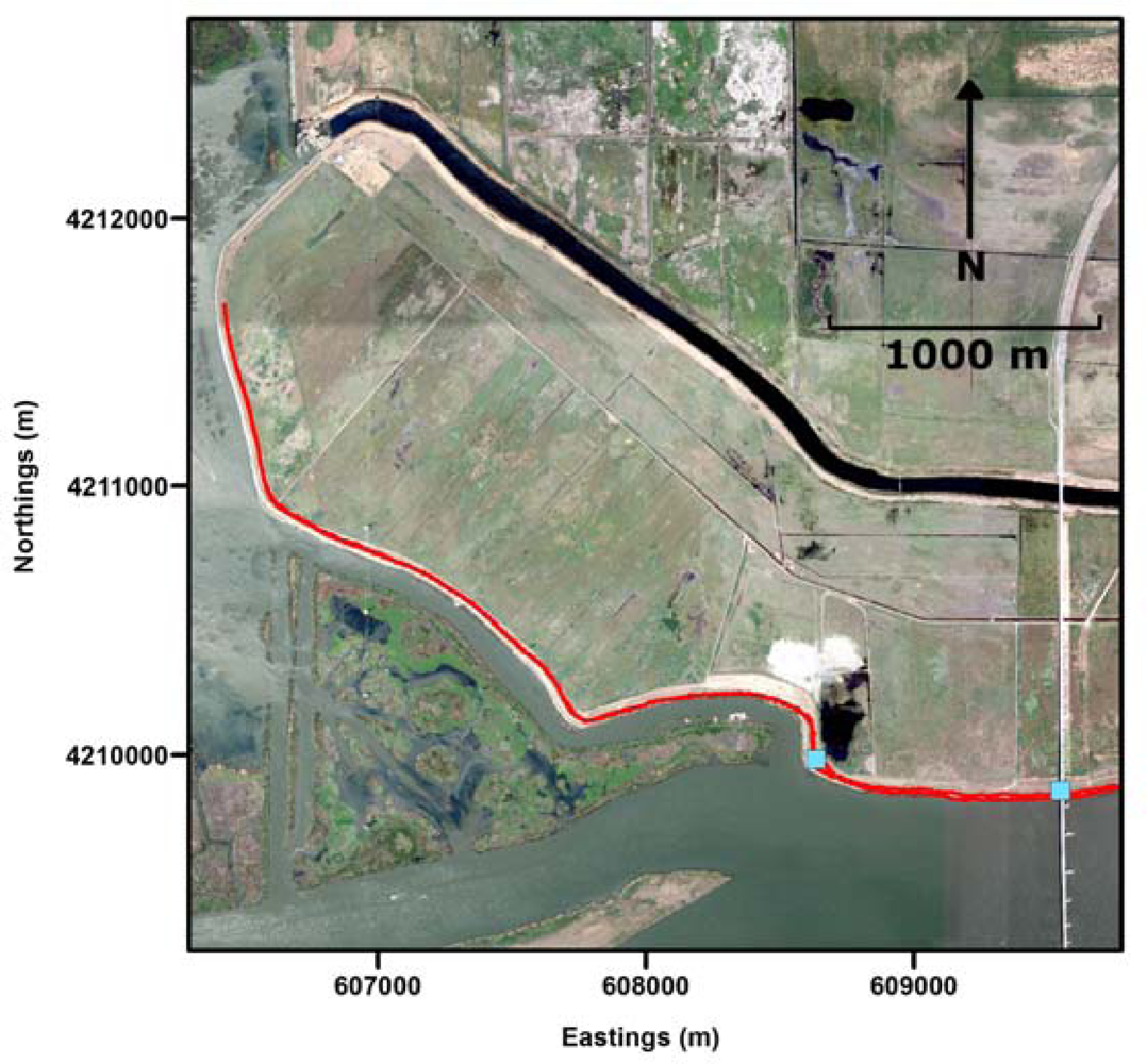
Figure 4 shows the area and extent (several kilometers) of the balloon testing on Sherman Island by displaying the GNSS trajectory of the balloon during LiDAR acquisition. For these tests, the balloon was tethered to a light duty pickup truck and pulled along the levee road at speeds between 7 and 15 km/h. For most of the survey, the balloon was at approximately 25 m above ground level. These survey parameters result in an observed ∼70 m LiDAR swath width, and a nominal point density (single pass) of 1,000 points/m2. Winds during the Sherman Island survey were sustained at approximately 15 knots, with periodic gusts up to 25 knots. The laser scanner rotation axis is maintained perpendicular to the flight direction by the sail attached to the balloon (see Figure 1).
Based upon the initial successful testing on Sherman Island, we attempted a more challenging effort designed to demonstrate the range and flexible deployment characteristics of this platform. After deflating the balloon, we mobilized within several hours, replenished the Helium supply, and transited over 250 miles. After a dusk reconnaissance and evening of no activity, we began at dawn to re-inflate the balloon and scan along a well-known section of the San Andreas Fault near Wallace Creek on the Carrizo Plain [26]. This test was designed principally as a simulation of a rapid-response in the immediate hours after a surface-rupturing earthquake along the San Andreas Fault. Furthermore, tests were used to evaluate the system’s suitability for high resolution mapping in environmentally sensitive or remote regions.
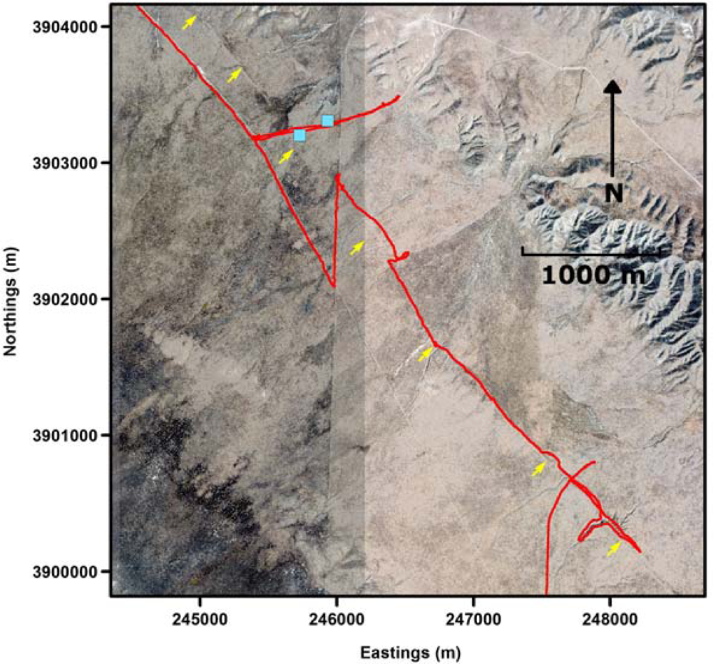
For the Carrizo Plain tests, the system was operated in both balloon and backpack mode. Figure 5 shows the GPS trajectory of the balloon (several kilometers), along with the site of the backpack tests (near the TLS marks) in relationship to the San Andreas Fault. For the Carrizo balloon tests, the three person crew took advantage of very calm wind conditions to untether the balloon from the pickup truck and walk the balloon LiDAR system along the fault rupture at a speed of approximately 3 km per hour. Note that the Carrizo plain is an extremely arid region that is very environmentally sensitive. As a result, any vehicles (including ATVs) are not allowed off-road along the actual fault scarp. Therefore, a walking balloon survey was required to provide minimal environmental impact. For most of the survey, the balloon was at approximately 30 meters above ground level. These survey parameters result in approximately an observed ∼80 meter LiDAR swath width, and a nominal point density (single pass) of 3,000 points/m2. For the backpack tests the instrument package was only 1 meter above the ground, with an observed swath width of approximately 4 meters, and a nominal point density of approximately 10,000 points/m2.
It should be noted that the high observed point densities returned for each of the system tests above represents an oversampling of the terrain due to the finite size of the laser cone of diffraction on the ground. For example, from a 25 m elevation the laser spot size on the ground for the Velodyne 32E is nominally 7 cm, which would imply that sampling at greater than 7 cm point spacing (or approximately 200 pts/m2) would result in overlapped LiDAR returns. Therefore, the test summary table below (Table 6), not only lists the observed point density, but also gives the theoretical highest point density that could be obtained without oversampling based on the expected laser spot size (denoted as maximum).
4.1. Control Dataset Description
In order to evaluate the accuracy of the data acquired with the prototype system, we acquired terrestrial laser scanning (TLS) data at four sites—two on Sherman Island (shown as cyan squares in Figure 4) and two on the Carrizo Plain (shown in Figure 5). The scans were acquired at approximately 1 cm point spacing (at a nominal 25 m range) using a Riegl VZ-400 scanner. The TLS point clouds were independently georeferenced to the same geodetic datum as the balloon LiDAR surveys with redundant GPS positioned retro-reflective targets. Post adjustment of the TLS data to the target points shows 1–2 cm level RMS agreement, which gives an overall indication of the quality of the TLS observations.
5. Results
5.1. Vertical Accuracy Assessment
To confirm the accuracy of the prototype system data (in both balloon and backpack modes) the resultant point clouds from the system were compared with results from the four TLS scans described in Section 4.1. For each of the TLS control sites, the kinematic system data were gridded at 1 meter interval over 100 m by 100 m sample sites to give approximately 10,000 observations. The sample sites were chosen in areas of bare earth, and therefore no filtering or classification was applied to either the TLS or balloon LiDAR data. The gridded balloon elevations were determined using TIN interpolation on the balloon LiDAR point cloud. Elevations at each of these grid points were then computed using TIN interpolation on the TLS point cloud and compared to the balloon LiDAR elevations. Statistics of the comparisons for all sites in both prototype system modes are given in Table 7.
The results in Table 7 clearly show that the TLS data, and the airborne kinematic data agree at a level of approximately 4–5 cm (1σ) in the vertical component. The backpack dataset shows slightly better agreement, at approximately 3 cm (1σ). As expected the backpack configuration performs slightly better. This is due to the decreased effect of IMU orientation angle errors at the smaller scan ranges from the backpack, as compared with the balloon mounted system. Considering that the expected ranging accuracy of the Velodyne scanner is quoted as 2 cm, and that the TLS point cloud target residuals during georeferencing were in the 1–2 cm range, it would appear that the elevation differences given in Table 7 are at or very near the overall expected noise level. These are very encouraging results, and show that the prototype kinematic system is capable of collecting accurately geolocated and very precise topographic information. The absence of a significant mean offset between the balloon/backpack data is also a good indication that the relative lever-arms and boresight angles have been well-estimated by the calibration procedure. These results are significantly better than those presented in [14], where a vertical standard deviation of 9.2 cm with respect to GPS control points was reported. The significantly better results are not surprising, given the more accurate laser, and higher accuracy IMU used in the system presented herein. The vertical results are also comparable to those given in [28] for a mobile system with a higher precision laser scanner.
5.2. Horizontal Accuracy Assessment
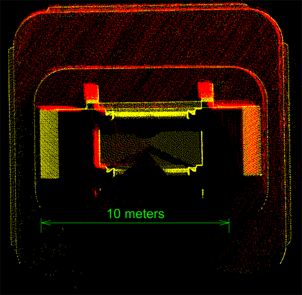
The TLS data acquired can also be used as a check on the horizontal accuracy of the described system. However, unfortunately, for a horizontal analysis, three of the four TLS point clouds acquired were of limited use because they were in areas that were mainly devoid of features suitable for checking horizontal accuracy. One of the TLS scans (Sherman 2), however, was captured around and under a bridge on Sherman Island (see lower left corner of Figure 4). This set of TLS data had enough identifiable features to enable a horizontal assessment of the balloon-based dataset. Concrete pillars and footing near the bridge (including those from an older abandoned bridge) gave several good hard surfaces for comparison (see Figure 6). As most of these target surfaces were vertical, a plane-based approach was used to estimate horizontal error. Small sections of point cloud data (1m by 1m) of the same hard surface in both the TLS data and the balloon data were extracted. A best-fit plane was then determined for each point cloud independently. The horizontal error was then given as the distance to the intersection point with the balloon data plane along the normal vector from the TLS plane centroid. The results of the comparisons for the set of 20 planar surfaces are given below in Table 8.
The results in Table 8 show that the horizontal accuracy of the balloon LiDAR data is approximately 17 cm horizontally. It is interesting to note that the horizontal errors of the balloon data are in general smaller near nadir, and are larger at the edges of the balloon swath. This clearly shows the effect of the wider beam divergence of the laser, the obliqueness that the laser pulse strikes the ground nearer to the swath edges and the accuracy of the IMU attitude determination. Overall, the horizontal errors are almost a factor of 4 larger than the vertical results presented in Table 7. As discussed in [20], this poorer horizontal performance is to be expected given the larger beam divergence and accuracy of the IMU, but is still within the desired goal of 20 cm horizontal accuracy (1σ).
5.3. Data Examples
Both the Carrizo Plain and Sherman Island datasets were collected for more than just testing of the prototype system; both of these areas had science and engineering questions that the research team felt could be addressed by a successful balloon based data collection. For the Carrizo plain, the goal was to identify small offset channels that previously had not been identified. For Sherman Island, the goal was to measure subsidence of the levee surrounding the island. Both sites had previously been surveyed with high resolution airborne LiDAR, Carrizo Plain in 2005 as part of the B4 project [29], and Sherman Island in 2007 as part of the Sacramento River delta acquisition [30]. This allowed a unique opportunity to compare the balloon LiDAR data to the existing data, and a baseline dataset to use on Sherman Island to attempt to measure subsidence.
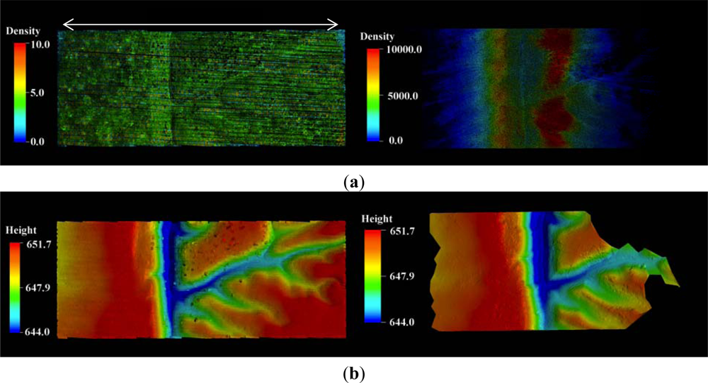
Figure 7 compares the B4 airborne LiDAR data on the Carrizo Plain with that collected by the balloon LiDAR system. Figure 7(a) shows that the balloon LiDAR data has a significantly higher point density (1,000 times higher). This is due to the low forward velocity (3 km/h) and low flight elevation (25 m), for the balloon LiDAR during data acquisition. Figure 7(b) clearly shows that the higher resolution data also illuminates additional subtle elevation changes in this section of the fault. We have found that the existing B4 data cannot be gridded at a resolution higher than 25 cm without noticeable gridding artifacts appearing. The balloon data however has been gridded successfully at 10 cm resolution with no noticeable gridding artifacts. We are hopeful this increased resolution will allow the identification of new faulting features along this portion of the San Andreas Fault.
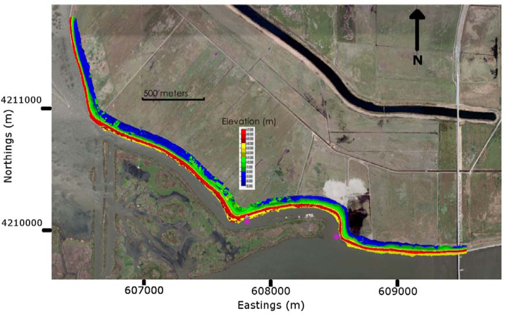
Figure 8 shows a DEM, color coded by elevation, produced using the balloon LiDAR data acquired on Sherman Island, CA. It is interesting to note that even though there were substantial (15–25 knot) winds during the survey, the field team was still able to acquire a dataset with almost complete coverage of the levee from the waterline to the toe of the inland slope of the levee for the entire surveyed section of the levee (>4 km long) in less than two hours. Asterisks notate the two areas where small segments of the levee were not captured.
6. Conclusions
The compact mobile laser scanning system has been successfully tested both deployed in a backpack and on a tethered balloon and highlight the required flexibility of the platform for a variety of remote sensing modalities. An accuracy assessment of the LiDAR data acquired with the system, compared to terrestrial laser scanning data gave a vertical accuracy for the point cloud of approximately 4 cm (1σ) in balloon mode, and 3 cm (1σ) in backpack mode while horizontal accuracy was approximately 17 cm (1σ) for the balloon tests. Raw LiDAR point densities with the system ranged from 1,000 pts/m2 in balloon mode to 10,000 pts/m2 in backpack mode. These accuracy and density values meet the stringent requirements of our target science and engineering applications, which require both high accuracy (vertical accuracy <10 cm, horizontal accuracy <20 cm (1σ)), and high point densities (>10 pts/m2).
7. Future Work
In the near future we plan to present the analysis of subsidence at the Sherman Island site, and the identification of new faulting features along the San Andreas Fault on the Carrizo Plain in additional publications. Tests of the system in other configurations (ATV mounted, helicopter UAV) for a number of applications are also planned for the near future. We have also begun planning and design of a second-generation system. Enhancements will improve its performance under tree canopy and in urban canyons (upgrade of IMU accuracy), and significantly reduce the overall system mass (to under 8 kg) by replacing the power sources with more compact batteries and by exchanging the current off-the-shelf GNSS receivers with OEM boards, along with building a suitable embedded computing module to replace the current ruggedized tablet computer. We also plan to add a wireless download link to allow near real-time monitoring of the acquired high-resolution datasets.
Acknowledgments
This work was funded by the Public Interest Energy Research (PIER) program of the California Energy Commission, grant 500-09-035 to the School of Ocean and Earth Sciences and Technology at the University of Hawaii. We thank Juan Mercado, Joel McElroy, and board members of Reclamation District #341, for graciously enabling the field tests on Sherman Island. We thank John Hurl, Kathy Sharum and Ryan Cooper of the Bureau of Land Management for Carrizo Plain access. We thank Sara Looney, David Phillips, and Chris Walls of UNAVCO for providing the high rate GPS observations from the PBO GPS stations and Dan Determan, Aris Aspiotes and Keith Stark for providing the high rate GPS observations from the USGS GPS stations. Finally, the authors would also like to thank Ralph Haugerud and Brian Sherrod of USGS and three anonymous reviewers for appraising an earlier version of the text. Their detailed and constructive criticisms have helped improved the overall manuscript.
References and Notes
- Shrestha, R.L.; Carter, W.E.; Lee, M.; Finer, P.; Sartori, M. Airborne laser swath mapping: accuracy assessment for surveying and mapping applications. J. Am. Congress Surv. Map 1999, 59, 83–94. [Google Scholar]
- Haugerud, R.A.; Harding, D.J.; Johnson, S.Y.; Harless, J.L.; Weaver, C.S.; Sherrod, B.L. High-resolution LIDAR topography of the Puget Lowland, Washington. GSA Today 2003, 13, 4–10. [Google Scholar]
- Carter, W.E.; Shrestha, R.L.; Slatton, K.C. Geodetic laser scanning. Phys. Today 2007, 60, 41–47. [Google Scholar]
- Maune, D.F. Digital Elevation Model Technologies and Applications: The DEM Users Manual, 2nd ed.; American Society for Photogrammetry and Remote Sensing: Bethesda, MD, USA, 2007. [Google Scholar]
- Chase, A.F.; Chase, D.Z.; Weishampel, J.F.; Drake, J.B.; Shrestha, R.L.; Slatton, K.C.; Awe, J.J.; Carter, W.E. Airborne LiDAR, archaeology, and the ancient Maya landscape at Caracol Belize. J. Archaeol. Sci 2011, 38, 387–398. [Google Scholar]
- Shrestha, R.L.; Carter, W.E.; Sartori, M.; Luzum, B.; Slatton, C. Airborne laser swath mapping: Quantifying changes in sandy beaches over time scales of weeks to years. ISPRS J. Photogramm 2005, 59, 222–232. [Google Scholar]
- Starek, M.J.; Slatton, K.C.; Shrestha, R.L.; Carter, W.E. Airborne Lidar Measurements to Quantify Change in Sandy Beaches. In Laser Scanning for the Environmental Sciences; Heritage, G., Large, A., Eds.; Wiley: Hoboken, NJ, USA, 2009; pp. 147–164. [Google Scholar]
- Maidment, D.; Edelman, S.; Heiberg, E.; Jensen, J.; Maune, D.; Schuckman, K.; Shrestha, R. Elevation Data for Floodplain Mapping; The National Academies Press: Washington, DC, USA, 2007. [Google Scholar]
- Hudnut, K.W.; Borsa, A.; Glennie, C.; Minster, J.B. High-resolution topography along surface rupture of the 16 October 1999 Hector Mine, California, earthquake (Mw 7.1) from airborne laser swath mapping. Bull. Seismol. Soc. Am 2002, 92, 1570–1576. [Google Scholar]
- Prentice, C.S.; Crosby, C.J.; Whitehill, C.S.; Arrowsmith, J.R.; Furlong, K.P.; Phillips, D.A. Illuminating northern California’s active faults. Trans. AGU EOS 2009, 90, 55–56. [Google Scholar]
- Zielke, O.; Arrowsmith, J.R.; Grant-Ludwig, L.B.; Akciz, S.O. Slip in the 1857 and earlier large earthquakes along the Carrizo Plain, San Andreas Fault. Science 2010, 327, 1119–1122. [Google Scholar]
- Blisniuk, K.; Rockwell, T.; Owen, L.A.; Oskin, M.; Lippincott, C.; Caffee, M.W.; Dortch, J. 2010.. Late Quaternary slip rate gradient defined using high-resolution topography and 10Be dating of offset landforms on the southern San Jacinto Fault zone, California. J. Geophys. Res 2010, 115, B0841. [Google Scholar]
- Wallace, L.; Lucieer, A.; Watson, C.; Turner, D. Development of a UAV-LiDAR system with application to forest inventory. Remote Sens 2012, 4, 1519–1543. [Google Scholar]
- Jaakkola, A.; Hyyppä, J.; Kukko, A.; Yu, X.; Kaartinen, H.; Lehtomäki, M.; Lin, Y. A low-cost multi-sensoral mobile mapping system and its feasibility for tree measurements. ISPRS J. Photogramm 2010, 65, 514–522. [Google Scholar]
- Lin, Y.; Hyyppä, J.; Jaakkola, A. Mini-UAV-borne LIDAR for fine-scale mapping. IEEE Geosci. Remote Sens. Lett 2011, 8, 426–430. [Google Scholar]
- Nagai, M.; Shibasaki, R.; Kumagai, H.; Ahmed, A. UAV-borne 3-D mapping system by multisensor integration. IEEE Trans. Geosci. Remote. Sens 2009, 47, 701–708. [Google Scholar]
- Glennie, C.; Lichti, D.D. Static calibrations and analysis of the Velodyne HDL-64E S2 for high accuracy mobile scanning. Remote Sens 2010, 2, 1610–1624. [Google Scholar]
- Baltsavias, E.P. Airborne laser scanning: basic relations and formulas. ISPRS J. Photogramm 2010, 54, 199–214. [Google Scholar]
- Morin, K.W. Calibration of Airborne Laser Scanners. M.S. Thesis. University of Calgary, Calgary, AB, Canada, 2002. [Google Scholar]
- Glennie, C. Rigorous 3D error analysis of kinematic scanning LIDAR systems. J. Appl. Geod 2007, 1, 147–157. [Google Scholar]
- Glennie, C.; Lichti, D.D. Temporal stability of the Velodyne HDL-64E S2 scanner for high accuracy scanning Applications. Remote Sens 2011, 3, 539–553. [Google Scholar]
- Filin, S. Recovery of systematic biases in laser altimetry data using natural surfaces. Photogramm. Eng. Remote Sensing 2003, 69, 1235–1242. [Google Scholar]
- Skaloud, J.; Lichti, D.D. Rigorous approach to bore-sight self-calibration in airborne laser scanning. ISPRS J. Photogramm 2006, 61, 47–59. [Google Scholar]
- Glennie, C. Calibration and kinematic analysis of the Velodyne HDL-64E S2 Lidar sensor. Photogramm. Eng. Remote Sensing 2012, 78, 339–347. [Google Scholar]
- Plate Boundary Observatory. Available online: http://pbo.unavco.org/ (accessed on 01 December 2012).
- Sieh, K.; Jahns, R.H. Holocene activity of the San Andreas Fault at Wallace Creek. Geol. Soc. Am. Bull 1984, 95, 883–896. [Google Scholar]
- USGS National Map Viewer. Available online: http://viewer.nationalmap.gov (accessed on 22 November 2012).
- Vaaja, M.; Hyyppä, J.; Kukko, A.; Kaartinen, H.; Hyyppä, H.; Alho, P. Mapping topography changes and elevation accuracies using a mobile laser scanner. Remote Sens 2011, 3, 587–600. [Google Scholar]
- Bevis, M.; Hudnut, K.; Sanchez, R.; Toth, C.; Grejner-Brzezinska, D.; Kendrick, E.; Caccamise, D.; Raleigh, D.; Zhou, H.; Shan, S.; et al. The B4 Project: Scanning the San Andreas and San Jacinto Fault Zones. Presented at American Geophysical Union-Fall Meeting 2005, San Francisco, CA, USA, December 2005; p. H34B-01.
- Joel Dudas, P.E. Delta LiDAR. California Surveyor 2009, 158, 10–17. [Google Scholar]


| Sensor | 32 lasers |
| 360° (azimuth) by 40° (vertical) FOV | |
| range: Up To 100 m | |
| 2 cm range accuracy (1σ) | |
| 0.09° Horizontal Encoder Resolution | |
| 5–15 Hz Rotation Rate (User Programmable) | |
| >700 kHz | |
| 25 W | |
| 2 kg | |
| 15 cm (height) by 8.5 cm (diameter) | |
| Laser | Class 1 |
| 905 nm wavelength | |
| 5 nanosecond pulse | |
| 2.79 mrad beam divergence (rectangular beam) | |
| Gyro Bias | 2°/h |
| Real-time Roll/Pitch Accuracy | 0.03° (1σ) |
| Real-time Heading Accuracy | 0.1° (1σ) |
| Gyro Dynamic Range | 100°/s |
| Measurement Rate | 100 Hz |
| Power Requirments | 15 W (9–18 V DC) |
| Weight | 2.2 kg |
| Dimensions | 23.4 × 12.0 × 8.0 (cm) |
| Residual (m) | Factory Calibration | Additional Interior Calibration |
|---|---|---|
| Minimum | −0.096 | −0.078 |
| Maximum | 0.098 | 0.076 |
| RMSE | 0.019 | 0.015 |
| Final Value | Estimated Standard Deviation | |
|---|---|---|
| Roll Offset (deg.) | −91.2328 | 0.0012 |
| Pitch Offset (deg.) | −2.2839 | 0.0012 |
| Heading Offset (deg.) | 90.0407 | 0.0026 |
| X Lever Arm (meters) | 0.1074 | 0.0008 |
| Y Lever Arm (meters) | −0.1256 | 0.0014 |
| Minimum (m) | −0.4507 |
| Maximum (m) | 0.4497 |
| Standard Deviation (m) | 0.0901 |
| RMSE (m) | 0.0903 |
| Test Site | Platform | Height (m) | Collection Speed (km/hr) | Swath Width (m) | Point Density (Observed/Maximum) | Laser Spot Size on Ground (cm) | Wind Speed (knots) |
|---|---|---|---|---|---|---|---|
| Sherman Island | Balloon/Truck | 25 | 7–15 | 70 | 1,000/200 | 7.0 | 15–25 |
| Carrizo Plain | Balloon/Walking | 30 | 3 | 80 | 3,000/140 | 8.4 | <5 |
| Carrizo Plain | Backpack | 1 | 3 | 4 | 10,000/2,500 | 2.0 | <5 |
| (Meters) | Min | Max | Average Magnitude | Mean | RMS | Standard Deviation |
|---|---|---|---|---|---|---|
| Balloon Configuration | ||||||
| Carrizo 1 | −0.1198 | 0.1336 | 0.0309 | −0.0042 | 0.0375 | 0.0373 |
| Carrizo 2 | −0.1267 | 0.1470 | 0.0369 | 0.0063 | 0.0459 | 0.0455 |
| Sherman 1 | −0.0703 | 0.1311 | 0.0327 | −0.0032 | 0.0403 | 0.0402 |
| Sherman 2 | −0.1200 | 0.1315 | 0.0378 | 0.0017 | 0.0472 | 0.0472 |
| Backpack Configuration | ||||||
| Carrizo 1 | −0.0815 | 0.0943 | 0.0226 | −0.0098 | 0.0284 | 0.0267 |
| Carrizo 2 | −0.0614 | 0.1012 | 0.0218 | 0.0088 | 0.0299 | 0.0286 |
| Minimum (m) | 0.0708 |
| Maximum (m) | 0.2344 |
| Mean Difference (m) | 0.1624 |
| Standard Deviation (m) | 0.0483 |
| RMSE (m) | 16.8903 |
Share and Cite
Glennie, C.; Brooks, B.; Ericksen, T.; Hauser, D.; Hudnut, K.; Foster, J.; Avery, J. Compact Multipurpose Mobile Laser Scanning System — Initial Tests and Results. Remote Sens. 2013, 5, 521-538. https://doi.org/10.3390/rs5020521
Glennie C, Brooks B, Ericksen T, Hauser D, Hudnut K, Foster J, Avery J. Compact Multipurpose Mobile Laser Scanning System — Initial Tests and Results. Remote Sensing. 2013; 5(2):521-538. https://doi.org/10.3390/rs5020521
Chicago/Turabian StyleGlennie, Craig, Benjamin Brooks, Todd Ericksen, Darren Hauser, Kenneth Hudnut, James Foster, and Jon Avery. 2013. "Compact Multipurpose Mobile Laser Scanning System — Initial Tests and Results" Remote Sensing 5, no. 2: 521-538. https://doi.org/10.3390/rs5020521
APA StyleGlennie, C., Brooks, B., Ericksen, T., Hauser, D., Hudnut, K., Foster, J., & Avery, J. (2013). Compact Multipurpose Mobile Laser Scanning System — Initial Tests and Results. Remote Sensing, 5(2), 521-538. https://doi.org/10.3390/rs5020521