Analysis of MODIS LST Compared with WRF Model and in situ Data over the Waimakariri River Basin, Canterbury, New Zealand

Abstract
:1. Introduction
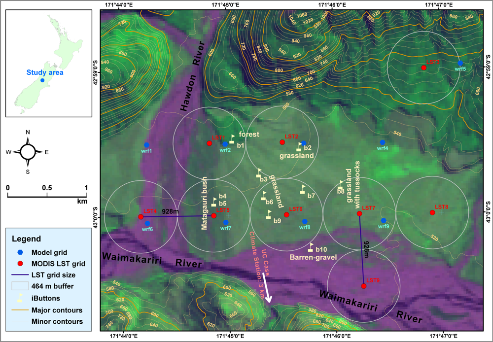
2. Study Area
3. Data
4. Methods
4.1. LST Pre-Processing
4.2. Spectral Unmixing
4.3. Spatial Overlay of MODIS LST, WRF Simulations and in situ Points
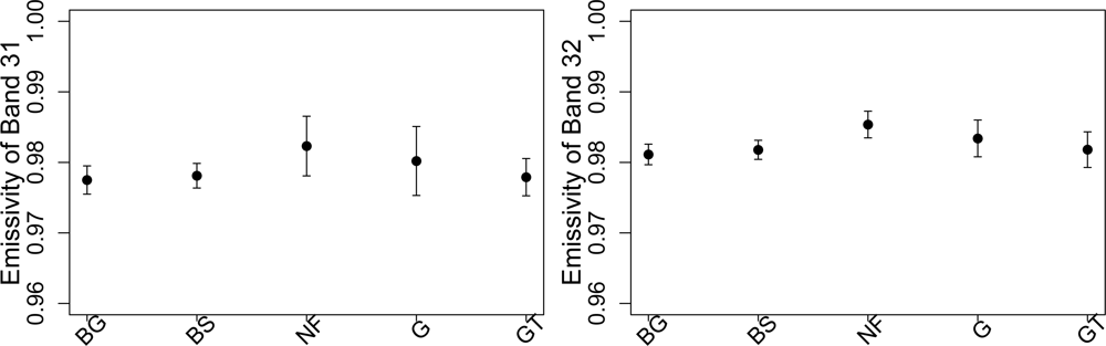
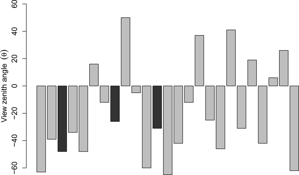
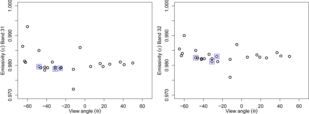
4.4. View Angle and Emissivity Analysis
4.5. Geo-Statistical Analysis
5. Results
5.1. Time-Series of Spatially Averaged Datasets
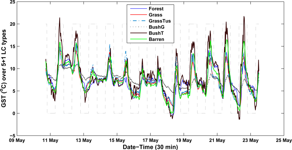
5.2. Land-Cover Based Time-series
5.3. Comparison between Day and Night Measurements
6. Discussion
6.1. Site-Specific Characteristics
6.2. Issues in LST Retrieval
7. Conclusions
Acknowledgments
References
- Wan, Z.; Dozier, J. A generalized split-window algorithm for retrieving land-surface temperature from space. IEEE Trans. Geosci. Remote Sens 1996, 34, 892–905. [Google Scholar]
- Jin, M. Analysis of land skin temperature using AVHRR observations. Bull. Am. Meteorol. Soc 2004, 85, 587–600. [Google Scholar]
- Coll, C.; Caselles, V.; Galve, J.M.; Valor, E.; Niclòs, R.; Sánchez, J.M.; Rivas, R. Ground measurements for the validation of land surface temperatures derived from AATSR and MODIS data. Remote Sens. Environ 2005, 97, 288–300. [Google Scholar]
- Trigo, I.; Monteiro, I.; Olesen, F.; Kabsch, E. An assessment of remotely sensed land surface temperature. J. Geophys. Res 2008, 113, D17108. [Google Scholar]
- Tang, B.; Bi, Y.; Li, Z.L.; Xia, J. Generalized split-window algorithm for estimate of land surface temperature from chinese geostationary fengyun meteorological satellite (FY-2C) data. Sensors 2008, 8, 933–951. [Google Scholar]
- Neteler, M. Estimating daily land surface temperatures in mountainous environments by reconstructed MODIS LST data. Remote Sens 2010, 2, 333–351. [Google Scholar]
- Ghent, D.; Kaduk, J.; Remedios, J.; Ardö, J.; Balzter, H. Assimilation of land surface temperature into the land surface model JULES with an ensemble Kalman filter. J. Geophys. Res 2010, 115, D19112. [Google Scholar]
- Trigo, I.; Dacamara, C.; Viterbo, P.; Roujean, J.; Olesen, F.; Barroso, C.; Camacho-de Coca, F.; Carrer, D.; Freitas, S.; Garcia-Haro, J.; et al. The satellite application facility for land surface analysis. Int. J. Remote Sens 2011, 32, 2725–2744. [Google Scholar]
- Dash, P.; Göttsche, F.M.; Olesen, F.S.; Fischer, H. Separating surface emissivity and temperature using two-channel spectral indices and emissivity composites and comparison with a vegetation fraction method. Remote Sens. Environ 2005, 96, 1–17. [Google Scholar]
- Huang, C.; Li, X.; Lu, L. Retrieving soil temperature profile by assimilating MODIS LST products with ensemble Kalman filter. Remote Sens. Environ 2008, 112, 1320–1336. [Google Scholar]
- Sheng, J.; Wilson, J.P.; Lee, S. Comparison of land surface temperature (LST) modeled with a spatially-distributed solar radiation model (SRAD) and remote sensing data. Environ. Model. Softw 2009, 24, 436–443. [Google Scholar]
- Meng, C.L.; Li, Z.L.; Zhan, X.; Shi, J.C.; Liu, C.Y. Land surface temperature data assimilation and its impact on evapotranspiration estimates from the Common Land Model. Water Resour. Res 2009, 45, W02421. [Google Scholar]
- Mostovoy, G.V.; King, R.L.; Reddy, K.R.; Kakani, V.G.; Filippova, M.G. Statistical estimation of daily maximum and minimum air temperatures from MODIS LST data over the state of mississippi. Gisci. Remote Sens 2006, 43, 78–110. [Google Scholar]
- Colombi, A.; Michele, C.D.; Pepe, M.; Rampini, A. Estimation of daily mean air temperature from MODIS LST in alpine areas. EARSeL eProc 2007, 6, 38–46. [Google Scholar]
- Zhang, W.; Huang, Y.; Yu, Y.; Sun, W. Estimation of daily mean air temperature from MODISLST in alpine areas. Int. J. Remote Sens 2011, 32, 1–26. [Google Scholar]
- Wang, C.; Qi, J.; Moran, S.; Marsett, R. Soil moisture estimation in a semiarid rangeland using ERS-2 and TM imagery. Remote Sens. Environ 2004, 90, 178–189. [Google Scholar]
- Hain, C.R.; Crow, W.T.; Mecikalski, J.R.; Anderson, M.C.; Holmes, T. An intercomparison of available soil moisture estimates from thermal infrared and passive microwave remote sensing and land surface modeling. J. Geophys. Res 2011, 116, D15107. [Google Scholar]
- Cheng, K.; Su, Y.; Kuo, F.; Hung, W.; Chiang, J. Assessing the effect of landcover changes on air temperature using remote sensing images-A pilot study in northern Taiwan. Landsc. Urban Plan 2008, 86, 297–297. [Google Scholar]
- Wan, Z.; Zhang, Y.; Zhang, Q.; Li, Z. Quality assessment and validation of the MODIS global land surface temperature. Int. J. Remote Sens 2004, 25, 261–274. [Google Scholar]
- Wan, Z. New refinements and validation of the MODIS Land-Surface Temperature/Emissivity products. Remote Sens. Environ 2008, 112, 59–74. [Google Scholar]
- Wan, Z.; Li, Z. Radiance-based validation of the V5 MODIS land-surface temperature product. Int. J. Remote Sens 2008, 29, 5373–5395. [Google Scholar]
- Kabsch, E.; Olesen, F.; Prata, F. Initial results of the land surface temperature (LST) validation with the Evora, Portugal ground-truth station measurements. Int. J. Remote Sens 2008, 29, 5329–5345. [Google Scholar]
- Coll, C.; Galve, J.; Sanchez, J.; Caselles, V. Validation of landsat-7/etm+ thermal-band calibration and atmospheric correction with ground-based measurements. IEEE Trans. Geosci. Remote Sens 2010, 48, 547–555. [Google Scholar]
- Niclòs, R.; Galve, J.M.; Valiente, J.A.; Estrela, M.J.; Coll, C. Accuracy assessment of land surface temperature retrievals from MSG2-SEVIRI data. Remote Sens. Environ 2011, 115, 2126–2140. [Google Scholar]
- Karnieli, A.; Agam, N.; Pinker, R.T.; Anderson, M.; Imhoff, M.L.; Gutman, G.G.; Panov, N.; Goldberg, A. Use of NDVI and land surface temperature for drought assessment: merits and limitations. J. Clim 2010, 23, 618–633. [Google Scholar]
- Mostovoy, G.V.; Anantharaj, V.; King, R.L.; Filippova, M.G. Interpretation of the relationship between skin temperature and vegetation fraction: Effect of subpixel soil temperature variability. Int. J. Remote Sens 2008, 29, 2819–2831. [Google Scholar]
- Wan, Z.; Zhang, Y.; Zhang, Q.; Li, Z. Validation of the land-surface temperature products retrieved from Terra Moderate Resolution Imaging Spectroradiometer data. Remote Sens. Environ 2002, 83, 163–180. [Google Scholar]
- Rigo, G.; Parlow, E. Modelling the ground heat flux of an urban area using remote sensing data. Theor. Appl. Climatol 2007, 90, 185–199. [Google Scholar]
- Holden, Z.A.; Abatzoglou, J.T.; Luce, C.H.; Baggett, L.S. Empirical downscaling of daily minimum air temperature at very fine resolutions in complex terrain. Agric. Forest Meteorol 2011, 151, 1066–1073. [Google Scholar]
- Fitzgerald, W.B.; Fahmy, M.; Smith, I.J.; Carruthers, M.A.; Carson, B.R.; Sun, Z.; Bassett, M.R. An assessment of roof space solar gains in a temperate maritime climate. Energy Build 2011, 43, 1580–1588. [Google Scholar]
- Brooks, R.T.; Kyker-Snowman, T.D. Forest floor temperature and relative humidity following timber harvesting in southern New England, USA. Forest Ecol. Manag 2008, 254, 65–73. [Google Scholar]
- Gubler, S.; Fiddes, J.; Gruber, S.; Keller, M. Scale-dependent measurement and analysis of ground surface temperature variability in alpine terrain. Cryosphere Discuss 2011, 5, 307–338. [Google Scholar]
- Wan, Z. MODIS Land-Surface Temperature Algorithm Theoretical Basis Document: LST ATBD; Institute for Computational Earth System Science, University of California: Santa Barbara, CA, USA, 1999. [Google Scholar]
- Wan, Z.; Zhang, Y.; Li, Z.; Wang, R.; Salomonson, V.; Yves, A.; Bosseno, R.; Hanocq, J. Preliminary estimate of calibration of the moderate resolution imaging spectroradiometer thermal infrared data using Lake Titicaca. Remote Sens. Environ 2002, 80, 497–515. [Google Scholar]
- Wan, Z. Collection-5 MODIS Land Surface Temperature Products Users’ Guide; ICESS, University of California: Santa Barbara, CA, USA, 2009. [Google Scholar]
- Wolfe, R.E.; Saleous, N. 7 MODIS Land Products and Data Processing. In Earth Science Satellite Remote Sensing Volume 1: Science and Instruments; Qu, J.J., Gao, W., Kafatos, M., Murphy, R.E., Salomonson, V.V., Eds.; Tsinghua University Press-Springer: Beijing, China, 2006; pp. 110–122. [Google Scholar]
- NCAR. ARW Version 3 Modeling System User’s Guide; Mesoscale & Microscale Meteorology Division, National Center for Atmospheric Research: Boulder, CO, USA, 2011. [Google Scholar]
- Skamarock, W.C.; Klemp, J.B.; Dudhia, J.; Gill, D.O.; Barker, D.M.; Duda, M.G.; Huang, X.Y.; Wang, W.; Powers, J.G. NCAR Technical Note: A Description of the Advanced Research WRF Version 3; Mesoscale & Microscale Meteorology Division, National Center for Atmospheric Research: Boulder, CO, USA, 2008. [Google Scholar]
- Maussion, F.; Scherer, D.; Finkelnburg, R.; Richters, J.; Yang, W.; Yao, T. WRF simulation of a precipitation event over the Tibetan Plateau, China - an assessment using remote sensing and ground observations. Hydrol. Earth Syst. Sci 2011, 15, 1795–1817. [Google Scholar]
- Jin, J.; Miller, N.L.; Schlegel, N. Sensitivity study of four land surface schemes in the wrf model. Adv. Meteorol. 2010, 2010, 167436:1–167436:11. [Google Scholar]
- Chen, F.; Dudhia, J. Coupling an advanced land surface-hydrology model with the Penn State-NCAR MM5 modeling system. Part I: Model implementation and sensitivity. Mon. Wea. Rev 2001, 129, 569–585. [Google Scholar]
- Dudhia, J. Numerical study of convection observed during the winter monsoon experiment using a mesoscale two-dimensional model. J. Atmos. Sci 1989, 46, 3077–3107. [Google Scholar]
- Averbuch, A.; Zheludev, M. Two linear unmixing algorithms to recognize targets using supervised classification and orthogonal rotation in airborne hyperspectral images. Remote Sens 2012, 4, 532–560. [Google Scholar]
- Keshava, N.; Mustard, J.F. Spectral unmixing. IEEE Signal Process. Mag 2002, 19, 44–57. [Google Scholar]
- Pu, R.; Gong, P.; Michishita, R.; Sasagawa, T. Spectral mixture analysis for mapping abundance of urban surface components from the Terra/ASTER data. Remote Sens. Environ 2008, 112, 939–954. [Google Scholar]
- Souza, C., Jr; Firestone, L.; Silva, L.M.; Roberts, D. Mapping forest degradation in the Eastern Amazon from SPOT 4 through spectral mixture models. Remote Sens. Environ 2003, 87, 494–506. [Google Scholar]
- Wang, L.; Uchida, S. Use of linear spectral mixture model to estimate rice planted area based on MODIS data. Rice Sci 2008, 15, 131–136. [Google Scholar]
- Gnanadesikan, R.; Kettenring, J.R. Robust estimates, residuals, and outlier detection with multiresponse data. Biometrics 1972, 28, 81–124. [Google Scholar]
- Ben-Gal, I. Outlier Detection. In Data Mining and Knowledge Discovery Handbook: A Complete Guide for Practitioners and Researchers; Maimon, O., Rockach, L., Eds.; Kluwer Academic Publishers: Dordrecht, The Netherlands, 2005; pp. 1–16. [Google Scholar]
- Proy, C.; Tanré, D.; Deschamps, P. Evaluation of topographic effects in remotely sensed data. Remote Sens. Environ 1989, 30, 21–32. [Google Scholar]


| iButton | LC type | Description |
|---|---|---|
| b1 | Forest | Dense native Beech trees with ≈10 m canopy height |
| b2 | Grassland | Native grass-turf with ≈5 cm height |
| b3 | Grassland | ” |
| b4 | Matagauri bush/scrub | Native bush with ≈50% density and ≈1.5 m height |
| b5 | Matagauri bush/scrub | ” (this iButton was fixed on top of the bush) |
| b6 | Grassland | Native grass-turf with ≈5 cm height |
| b7 | Grassland | ” |
| b8 | Grassland with tussocks | ” mixed with native tussock with ≈20 cm height |
| b9 | Grassland | Native grass-turf with ≈5 cm height |
| b10 | Barren-gravel | Bare soil with gravel on the inactive river banks |
| LC-Types | LST1 | LST4 | LST5 | LST6 | LST7 | si |
|---|---|---|---|---|---|---|
| Barren-gravel | 0.35 | 0.70 | 0.10 | 0.15 | 0.10 | LST9 |
| Bush-scrub | 0.25 | 0.05 | 0.50 | 0.00 | 0.05 | LST5-6 |
| Forest | 0.25 | 0.00 | 0.00 | 0.00 | 0.00 | LST3 |
| Grassland | 0.15 | 0.20 | 0.40 | 0.85 | 0.10 | LST2 |
| Grass-Tussock | 0.00 | 0.05 | 0.00 | 0.00 | 0.75 | LST8 |
| Stat. | in situ | MODIS | WRF |
|---|---|---|---|
| μ | 8.49 | 6.98 | 7.99 |
| σ | 3.26 | 4.33 | 3.63 |
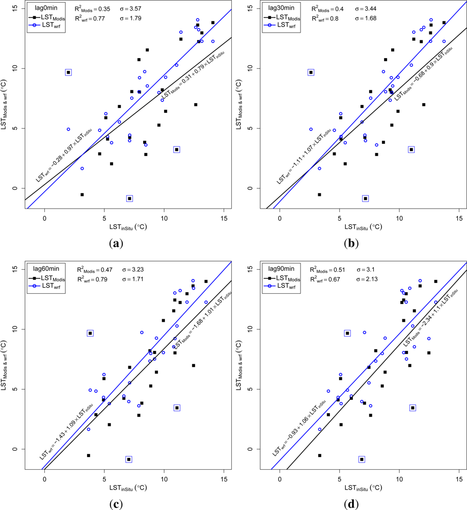
| MOD∼inSitu | WRF∼inSitu | MOD∼WRF | ||||||
| Time-Lag | R2 | σ | p-val. | F-Stat | R2 | σ | R2 | σ |
| 0min | 0.35 | 3.57 | 0.0020 | 12.36 | 0.77 | 1.79 | 0.56 | 2.92 |
| 30min | 0.40 | 3.44 | 0.0008 | 15.10 | 0.80 | 1.68 | 0.62 | 2.73 |
| 60min | 0.47 | 3.23 | 0.0002 | 20.20 | 0.79 | 1.71 | 0.60 | 2.80 |
| 90min | 0.51 | 3.10 | 0.0000 | 24.10 | 0.67 | 2.13 | 0.52 | 3.06 |
| (a) | ||||||||
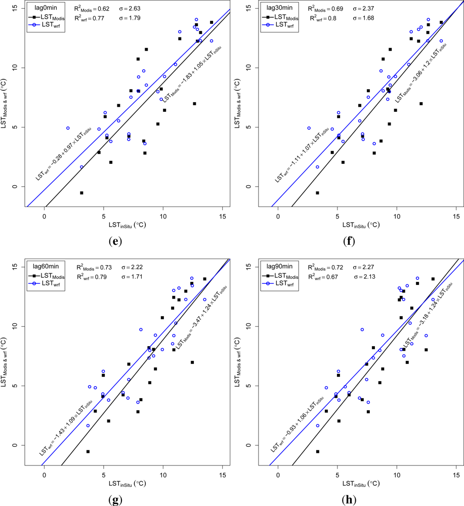
| MOD∼inSitu | WRF∼inSitu | MOD∼WRF | ||||||
| Time-Lag | R2 | σ | p-val. | F-Stat | R2 | σ | R2 | σ |
| 0min | 0.62 | 2.63 | 0.0000 | 32.84 | 0.77 | 1.79 | 0.69 | 2.38 |
| 30min | 0.69 | 2.37 | 0.0000 | 45.13 | 0.80 | 1.68 | 0.72 | 2.26 |
| 60min | 0.73 | 2.22 | 0.0000 | 54.55 | 0.79 | 1.71 | 0.67 | 2.47 |
| 90min | 0.72 | 2.27 | 0.0000 | 51.43 | 0.67 | 2.13 | 0.56 | 2.83 |
| (b) | ||||||||
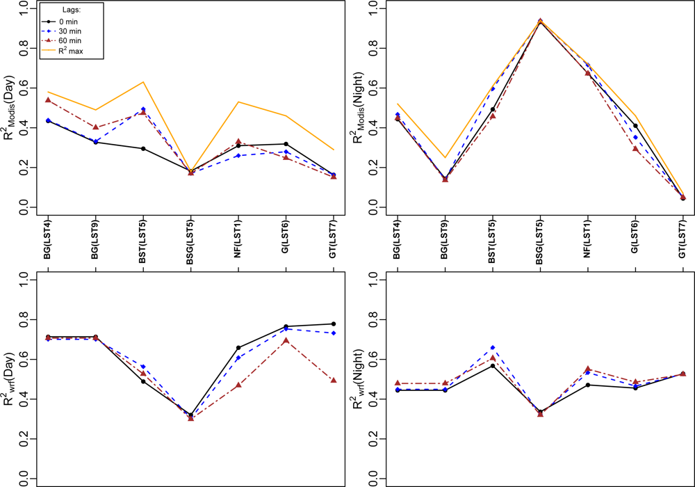
| LC-Type/R2@lag | MOD∼inSitu | WRF∼inSitu | MOD∼WRF | |||||
|---|---|---|---|---|---|---|---|---|
| 0 | 30 | 60 | best lag | 0 | 30 | 0 | 30 | |
| BarrenGravel(LST4) | 0.42 | 0.51 | 0.62 | 0.68(68) | 0.71 | 0.75 | 0.73 | 0.75 |
| BarrenGravel(LST9) | 0.38 | 0.43 | 0.50 | 0.56(69) | 0.71 | 0.75 | 0.43 | 0.46 |
| BushScrubT(LST5) | 0.51 | 0.62 | 0.66 | 0.77(19) | 0.67 | 0.74 | 0.65 | 0.67 |
| BushScrubG(LST5) | 0.04 | 0.07 | 0.09 | 0.18(74) | 0.31 | 0.33 | 0.65 | 0.67 |
| Forest(LST1) | 0.21 | 0.23 | 0.31 | 0.47(80) | 0.48 | 0.50 | 0.64 | 0.70 |
| Grassland(LST6) | 0.42 | 0.46 | 0.48 | 0.61(91) | 0.77 | 0.78 | 0.69 | 0.73 |
| GrassTussock(LST7) | 0.37 | 0.39 | 0.43 | 0.52(57) | 0.81 | 0.79 | 0.53 | 0.62 |
Share and Cite
Sohrabinia, M.; Rack, W.; Zawar-Reza, P. Analysis of MODIS LST Compared with WRF Model and in situ Data over the Waimakariri River Basin, Canterbury, New Zealand. Remote Sens. 2012, 4, 3501-3527. https://doi.org/10.3390/rs4113501
Sohrabinia M, Rack W, Zawar-Reza P. Analysis of MODIS LST Compared with WRF Model and in situ Data over the Waimakariri River Basin, Canterbury, New Zealand. Remote Sensing. 2012; 4(11):3501-3527. https://doi.org/10.3390/rs4113501
Chicago/Turabian StyleSohrabinia, Mohammad, Wolfgang Rack, and Peyman Zawar-Reza. 2012. "Analysis of MODIS LST Compared with WRF Model and in situ Data over the Waimakariri River Basin, Canterbury, New Zealand" Remote Sensing 4, no. 11: 3501-3527. https://doi.org/10.3390/rs4113501
APA StyleSohrabinia, M., Rack, W., & Zawar-Reza, P. (2012). Analysis of MODIS LST Compared with WRF Model and in situ Data over the Waimakariri River Basin, Canterbury, New Zealand. Remote Sensing, 4(11), 3501-3527. https://doi.org/10.3390/rs4113501