Simulations of Infrared Radiances over a Deep Convective Cloud System Observed during TC⁴: Potential for Enhancing Nocturnal Ice Cloud Retrievals

1. Introduction

Because of their influences on the Earth’s radiation budget and hydrological cycle, the need to monitor cloud properties from satellites has long been recognized in the study of climate (e.g., [1–5]). With the widespread availability of well-calibrated polar and geostationary orbiting satellite imagers, more sophisticated cloud parameterizations, maturing remote sensing algorithms, and faster computers, cloud properties sensed remotely from satellite imager data are also increasingly relevant for improving numerical weather forecasts (e.g., [6,7]). Because of their favorable spatial and temporal coverage, passive satellite measurements at solar and infrared (IR) measurements have been extensively used to retrieve optical and micro/macro physical properties of clouds. A wide variety of techniques have been developed to retrieve cloud properties using various combinations of those radiances measured by both operational and research satellite imagers such as the Moderate Resolution Imaging Spectroradiometer (MODIS). Most methods have focused on retrieving cloud properties, such as optical thickness τ and particle effective diameter D_e, during the daytime because reflected solar radiation can be used to retrieve the properties over nearly the full range of expected values (e.g., [4,8–13]). During both day and night, it is possible to estimate cloud top heights for the full range of cloud optical thicknesses (e.g., [5,14,15]), but retrievals of τ itself and D_e have been limited to optically thin (τ < ∼5) clouds because of the constraints of the blackbody limit (e.g., [10,16–24]). Thus, monitoring of cloud τ and D_e, parameters that determine the cloud water path CWP, using satellite solar and IR imagers is confined to daytime for the clouds that contribute the bulk of liquid and ice water to the atmospheric water budget.

The diurnal variations of both liquid and ice cloud properties are also important for understanding the Earth radiation and latent heat budgets. Accurately quantifying the diurnal variations of cloud properties then is crucial for improving climate models (e.g., [25–29]). Thus, retrieval of a full range of cloud properties during nighttime is essential for accurately defining their role in climate. Moreover, without that full range, assimilations of τ or CWP will produce diminished benefit to numerical weather predictions at night compared to those during the day. Mitigation of the blackbody limitation in cloud remote sensing, therefore, is an endeavor important for further validation and improvement of both weather and climate models.

To begin the process of addressing this challenge, this study investigates the IR signals from optically thick ice clouds using campaign measurements and rigorous radiative transfer modeling to determine the potential for estimating optically thick ice cloud τ and D_e using selected IR bands at 3.7, 6.7, 7.3, 8.5, 10.8, and 12.0 μm. These bands are among the channels on many geostationary and polar-orbiting meteorological satellite imagers. Section 2 describes the detailed measurements from the NASA ER-2 and DC-8 aircraft and radiosonde ascents for a case study of a tropical deep convective cloud system observed during the Tropical Composition, Cloud and Climate Coupling Experiment (TC⁴) [30]. The measurements include cloud vertical profiles made by a cloud radar and lidar, ice cloud particle sizes and habits from in situ probes, and radiances made by an airborne scanning spectrometer covering visible to IR bands and an airborne scanning high-resolution IR interferometer. Using observations and simulations, section 3 examines the effects of τ and D_e on upwelling IR radiances over the tropical deep convective cloud system. The measurements from the airborne scanning high-resolution IR interferometer are used to construct IR brightness temperatures at the MODIS bands of 3.7, 6.7, 7.3, 8.5, 10.8, and 12.0 μm. Simulations are based on a rigorous radiative transfer model with inputs of in situ atmospheric profiles and cloud microphysical and optical properties derived from airborne measurements. Gamma particle size distributions are also used in simulations for the aim of investigating the influence of D_e on IR radiances. Section 4 summarizes this study.

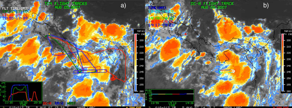
2. Combined Measurements over a Deep Convective Cloud System

This study focuses on a particular convective cloud system observed during the 5 August 2007 TC⁴ mission, when the ER-2 and DC-8 executed more than 4 hours of flights at their cruising altitudes of about 20 and 10 km, respectively. The coordinated flight segment between 1350 and 1438 UTC is the focus of this study.

Because of its high altitude, the ER-2 effectively serves as a satellite having an array of remote sensing instruments. The MODIS/Advanced Spaceborne Thermal Emission and Reflection Radiometer, ASTER Airborne Simulator (MASTER) on the ER-2 measured radiances at most of the satellite imager wavelengths of interest. The MASTER is a cross-track scanning spectrometer that measures reflected solar and emitted thermal radiation in 50 narrowband channels in the range 0.4–13 μm. Its 2.5-mrad instantaneous field of view (FOV) results in a spatial resolution at nadir of 50 m at the nominal ER-2 altitude of 20 km. At that altitude, the total FOV of the MASTER is 85.92°·(±42.96° from nadir), which yields a ground swath of about 37.25 km. The MASTER is described in detail by [31] and [32]. The IR radiances observed by MASTER bands 30 (3.7 μm), 43 (8.6 μm), 48 (11.3 μm), and 49 (12.2 μm) are used in this study.

During TC⁴ the MASTER lacked the water vapor bands at 6.7 and 7.3 μm that are currently carried on the MODIS. In this study, the measurements from the Scanning High-resolution Interferometer Sounder (S-HIS) on the ER-2 are used to construct radiances in the 6.7 and 7.3 μm bands that are available on the MODIS. The S-HIS is a scanning interferometer which measures emitted thermal radiation at high spectral resolution between 3.3 and 18 μm [33]. Its instrument FOV is 100 mrad and its total view angle is ±30°, so from the ER-2 it produces sounding data with 2 km resolution at the nadir and covers a 40-km ground swath.

The ER-2 carried the CRS and CPL, which are well suited for ice cloud studies because of their high sensitivities and spatial resolutions. The CRS [34] is a 94-GHz (W-band, 3.2-mm wavelength) pulsed polarimetric Doppler radar. It was designed to provide nadir cloud profiling from the ER-2. The ER-2 CRS measurements have a vertical resolution of 37.5 m and temporal resolution of 0.5 s. The minimum detectable reflectivity is −28 dBZ for the CRS at a range of 15 km from the ER-2. Thus, the CRS measurements could miss the tops of ice clouds with small ice particles. Lidar measurements are used to observe the clouds missed by the CRS since lidar is more sensitive to small ice particles and optically thin cirrus than radar. McGill et al. [35] found that the τ missed by the CRS, but detected by the CPL, is in the range of 0.15–0.45. The CPL is a backscatter lidar with three wavelengths of 0.355, 0.532, and 1.064 μm [36]. It scans downward from the ER-2 with a vertical resolution of 30 m and a 1-s temporal resolution, corresponding to ∼200 m at an average ER-2 ground speed of 200 ms⁻¹. Only the CPL measurements at 0.532 μm over the deep convective cloud system are used in this study.

The DC-8 carried several cloud particle size probes to take in situ measurements and dropsondes to obtain temperature and humidity profiles below the aircraft. Ice cloud bulk scattering properties are mainly dependent on ice particle habits and ice cloud particle size distributions. Combined measurements from the 2-Dimensional Stereo (2D-S) probe, 2D Cloud Imaging Probe (CIP), and Precipitation Imaging Probe (PIP) on the DC-8 are used to construct ice cloud particle size distributions covering size bins from 5 μm to 6 mm in the present study.

Numerous small ice particles (maximum dimension D less than 50 μm) have been observed in ice clouds by in situ measurements. However, large portions of these small ice particles could be generated by large crystals shattering on the inlets of instruments such as the Forward Scattering Spectrometer Probe (FSSP) and others which ingest ice particles into sample volumes through inlets ([37] and references therein). The 2D-S uses detector arms instead of an inlet tube to minimize shattering fragments from entering the sample volume, however, collisions of the ice crystals and the forward elements of the probe still introduce some significant uncertainties into the derived size distributions [38,39]. It detects particles as small as 10 μm (the minimum size bin is 5–15 μm) [38]. For the TC⁴ dataset, the maximum particle size bin that produced adequate sampling statistics was about 3000 μm.

The CIP measured particle sizes ranging from about 50–100 μm to more than 1 mm, and the PIP measured particles sizes from about 100 μm to 6 mm [40]. Although both instruments nominally provide a minimum detectable size of 50 μm, the lowest detection threshold from the CIP is 100 μm during TC⁴ because of uncertainties in the probe’s sample volume [40–42]. Jensen et al. found that the size distributions derived from the CIP agree well with those from the 2D-S imaging instruments for the size bins above 100–200 μm despite the uncertainties in both instruments’ sample volume sizes [37]. For detailed information on the CIP and PIP, see Tian et al. who investigated cirrus ice particle size distributions using TC⁴ CIP and PIP observations [42].

The Cloud Particle Imager (CPI) can image particles in the size range of 15–2,500 μm with a nominal 2.3-μm resolution [38]. During TC⁴, the CPI aboard the DC-8 had 33 size bins between 0 and 1,000 μm. The particle densities of seven habit categories including sphere, column, plate, rosette, budding rosette, small and large irregular particles were measured separately for ice particles with D < 50 μm and D > 50 μm. The habit mixtures derived with an automated technique from the measured number densities are used for computing ice cloud bulk scattering properties. Although all of the probe measurements have some significant uncertainties, they still provide the most realistic estimate of the microphysical properties of the clouds in this system and should yield reasonable radiances.

Figure 1 shows a combination of two Geostationary Operational Environmental Satellite, GOES-10 and GOES-12, 10.8-μm IR brightness temperature images over the TC⁴ domain at 1558 UTC, 5 August 2007. Coordinated flights of the ER-2 over and the DC-8 in the clouds followed an east-west orientation in the Panama Bight at about 6.5°N, where an anvil cirrus was observed flowing from a deep convective core at about 79°W. One coordinated segment for the ER-2 and DC-8 over the anvil cirrus and deep convective core occurred from about 13:50 to 14:40 UTC (ER-2 flight) which is shown in Figure 2(a) together with the MASTER false color RGB image. The MASTER pseudo-RGB image is based on the band 5 (0.66 μm) reflectance, band 21 (2.16 μm) reflectance, and band 48 (11 μm) reversed-scale brightness temperatures. The ocean background is dark in the false color image. Optically thick ice clouds including the anvil and the upper part of the deep convective core are purple. Thin cirrus clouds are light blue. Note that only the DC-8 tracks (in red) coordinated with the ER-2 track (in blue) are shown here. During the west-to-east leg, the DC-8 flight had a lag of about 7–8 min with respect to the ER-2, while along the east-to-west leg, the ER-2 lagged the DC-8 by about 6–7 min. Figure 2(b) shows the cloud vertical cross-section given by the CRS reflectivity along the ER-2 track. Cloud top and base detected by the CPL for the upper two ice cloud layers are also shown in Figure 2(b). The vertical structure of the CRS reflectivity distinctly shows the outflow anvil cirrus from the deep convection.

The DC-8 launched four dropsondes along the track shown in Figure 2: X1 at 79.49°W, 6.50°N at 13:54 UTC, X2 at 80.86°W, 6.19°N at 14:10 UTC, X3 at 79.68°W, 6.49°N at 14:23 UTC, and X4 at 81.37°W, 6.18°N at 14:42 UTC. Surface radiosonde measurements launched at 15:05 UTC at Las Tablas, Panama (80.25°W, 7.75°N) from the Nittany Atmospheric Trailer and Integrated Validation Experiment (NATIVE) included high vertical resolution profiles of atmospheric temperature, humidity, and ozone mixing ratio [43]. Figure 3 shows the mean profiles of atmospheric water vapor and temperature from the four DC-8 dropsondes and the profiles of temperature and water vapor from the NATIVE ground-based sonde. The mean temperature profile is essentially the same as that from the NATIVE sonde. The mean water vapor profile from the dropsondes is only available below about 10.3 km. Thus, above 10.3 km, the scaled NATIVE water vapor profile is used to complete the mean water vapor profile that is used for the present simulations together with the NATIVE temperature and ozone profiles. The dropsondes sampled two points, X1 and X3, within the convective column and two, X2 and X4, outside of it under the anvil. Because the NATIVE sounding was taken in air lacking a deep convective cloud, a second sounding, launched at 23:20 UTC, 4 August 2007 from Alajuela, Costa Rica (9.98°N, 84.21°W) when a convective system was overhead, was used to better represent the convective cloud conditions that would be encountered in the convective cloud. The Alajuela sounding is significantly moister above 14 km than its NATIVE counterpart.

3. Infrared Radiances over the Deep Convective Cloud System: Observations and Simulations

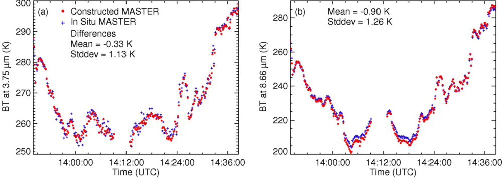
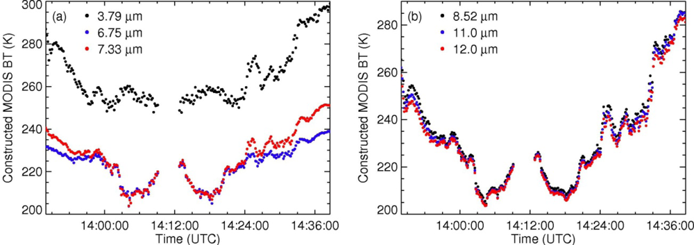
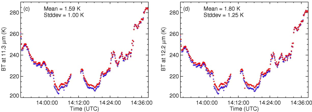
3.1. The S-HIS Derived IR Brightness Temperatures at the MODIS Bands

Although the MASTER has bands similar to the MODIS complement, it has different spectral response functions (SRFs) and lacks a few channels. In particular, it does not have the MODIS water vapor bands at 6.7 and 7.3 μm. Here, the measurements from the S-HIS aboard the ER-2 are used to construct the MODIS bands at 3.7, 6.7, 7.3, 8.5, 10.8, and 12.0 μm. Figure 4 shows an example of an S-HIS spectrum and the Aqua MODIS and TC⁴ MASTER band SRFs around 3.7, 6.7, 7.3, 8.5, 10.8, and 12.0 μm. The S-HIS measurements and MASTER SRFs at 3.7, 8.5, 10.8, and 12.0 μm were used to construct the pseudo-MASTER brightness temperatures, which were then compared to the corresponding observed MASTER brightness temperatures. The matched brightness temperatures, shown in Figure 5, agree well with each other with a standard deviation of ∼1 K in their differences. Theoretically, if S-HIS and MASTER have the exact same observation geometry and FOVs, the comparisons should be essentially the same. The biases are likely due to calibration differences, while the variability in the differences is probably the result of the two instruments’ viewing slightly different scenes because of differences in their pixel sizes. At a cloud-top height of 15 km, the MASTER FOV is only ∼12 m at nadir compared to 500 m for the S-HIS. Similarly, the S-HIS measurements and MODIS SRFs at 3.7, 6.7, 7.3, 8.5, 10.8, and 12.0 μm were used to simulate the MODIS-observed brightness temperatures at these bands (Figure 6). These pseudo-MODIS brightness temperatures are considered as MODIS observations in the present study.

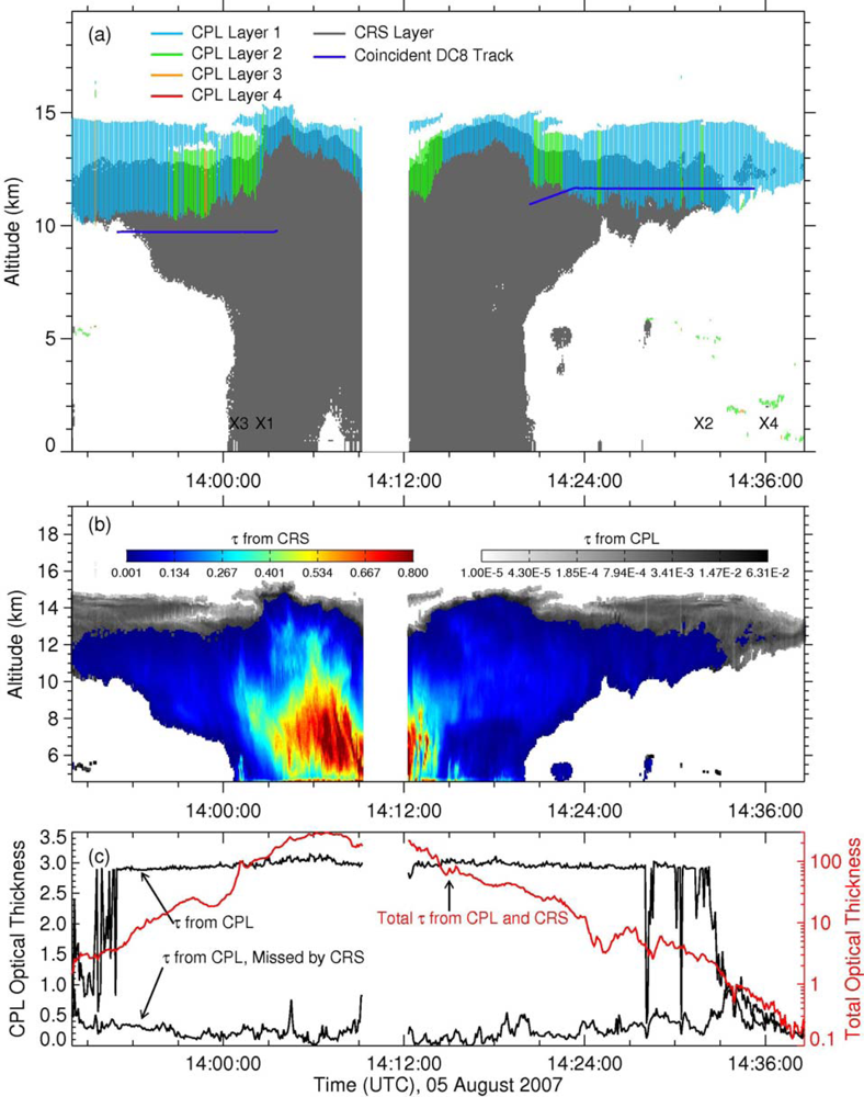
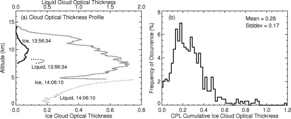
3.2. Optical Thickness Profiles from Combined CRS and CPL Measurements

The vertical profile of the cloud water content can have significant influence on outgoing IR radiances, even for optically thick clouds. A thick convective cloud with a low ice water content at the top will produce a different IR temperature than one having a dense top (e.g., [44]). A multilayered ice-over-liquid cloud will yield a different IR temperature than a single-layered ice cloud having the same cumulative optical depth. Thus, it is important to use a realistic vertical profile of the water content or optical depth in the simulations.

The CRS measurements are primarily used to obtain vertical cloud τ profiles at a resolution of 15 m. Three cloud phases, ice, liquid, and mixed phase, are considered here. The vertical profiles are separated into three layers, ice (top layer), mixed-phase (middle layer), and liquid (bottom layer) clouds. The layer with temperatures less than −20 °C is defined as ice cloud, the layer with temperature exceeding 0 °C is a liquid cloud. The layer between −20 °C to 0 °C is the mixed-phase cloud [45]. In the bottom layer, the liquid cloud water content (LWC) is computed as follows,

$$Z_e=57.54LW{C}^{5.17}$$

(1)

where LWC is in g·m⁻³ and Z_e is in mm⁶·m⁻³ [46]. In the ice cloud, the ice water content (IWC) is

$$IWC=0.137Z_e^{0.643}$$

(2)

where IWC and Z_e are in the same units as those for Z_e−LWC [47].

For the mixed-phase layer, LWC is assumed to decrease to 0 linearly with increasing altitude from the freezing level to the bottom of the ice cloud layer. Conversely, IWC is assumed to increase linearly from 0 g·m⁻³ following Equation (2). On the basis of these assumptions, an ice fraction IceFra is defined to separate the two parts of CRS reflectivity, IceFra = −(T − T₀)/(T₀ − T_Tra), where T is atmospheric temperature in degree, T₀ is the temperature at the freezing level, and T_Tra is the transition temperature from mixed-phase to ice cloud. In the present study, 0 °C is used for T₀, so IceFra = T/T_Tra. A phase transition temperature of −20 °C (altitude is ∼8.3 km) is used. Therefore, the two parts of the CRS reflectivity due to cloud ice $Z_e^{\mathit{ice}}$ and liquid water $Z_e^{\mathit{liq}}$, are obtained from $Z_e^{\mathit{ice}}=\mathit{IceFra}*Z_e$ and $Z_e^{\mathit{liq}}=\left(1-\mathit{IceFra}\right)*Z_e$, respectively. IWC and LWC are then obtained by applying ${\text{Z}}_{\text{e}}^{\text{liq}}$ and $Z_e^{\mathit{liq}}$ to Equations (1) and (2), respectively. Because of difficulties in separating the surface radar return from the hydrometeors within the first 500 m above the surface, CRS reflectivity below 500 m is assumed to be that at the level of 500 m [48,49].

While the CRS retrieval algorithm assumes the ice fraction varies as indicated above, the Rosemount icing probes detected no liquid water at temperatures up to −3 °C for this flight segment. Thus, to provide a more realistic variation of cloud water structure, a second profile was constructed assuming no liquid water for temperatures less than 0 °C. Thus, in the 0 to −20 °C transition zone used above, IceFra is set equal to 1.0 for a second set of calculations. Both results are used to determine the sensitivity of the calculations to the assumptions about supercooled liquid water in the clouds.

The CPL measurements are used to compensate for the optically thin cirrus part missed by the CRS measurements [35]. Figure 7 shows the vertical structure of the cloud system as seen from the CRS and CPL measurements and the 15-m resolution τ profiles constructed from the CRS and CPL data for the pure ice layer. The total optical thicknesses, those from the CPL and those missed by the CRS along the flight track over the cloud system, are also shown in Figure 7. Visible τ from the CRS shown in Figure 7(c) is derived from the empirical relationships, τ = 0.065·IWP^0.84 for cloud ice and τ = 3.0/20.0·LWP for cloud liquid (assuming water clouds with D_e = 20 μm and an extinction efficiency, Q_e = 2.0), respectively [50]. The water paths for each layer are the products of the water content and the 15-m thickness for each layer. The minimum detectable reflectance from the CRS is used to isolate the CPL-measured cloud areas missed by the CRS measurements: overlapping is denoted where the CRS gray region is visible under the CPL color region in Figure 7(a). The cloudy area missed by the CRS is shown as the gray region in Figure 7(b). Figure 8(a) shows examples of the constructed vertical profiles for 15-m layer ice and liquid cloud τ. One profile is from an anvil cloud measured at 13:56:34 UTC, and the other is taken from a convective core measured at 14:06:10 UTC. The CPL cumulative ice cloud τ missed by the CRS measurements along the flight path are detailed in Figure 8(b). The τ value most frequently missed by the CRS but detected by the CPL is ∼0.20. Overall, the average τ missed by the CRS is 0.28 ± 0.17, which is consistent with the values (0.15–0.45) deduced by [35].

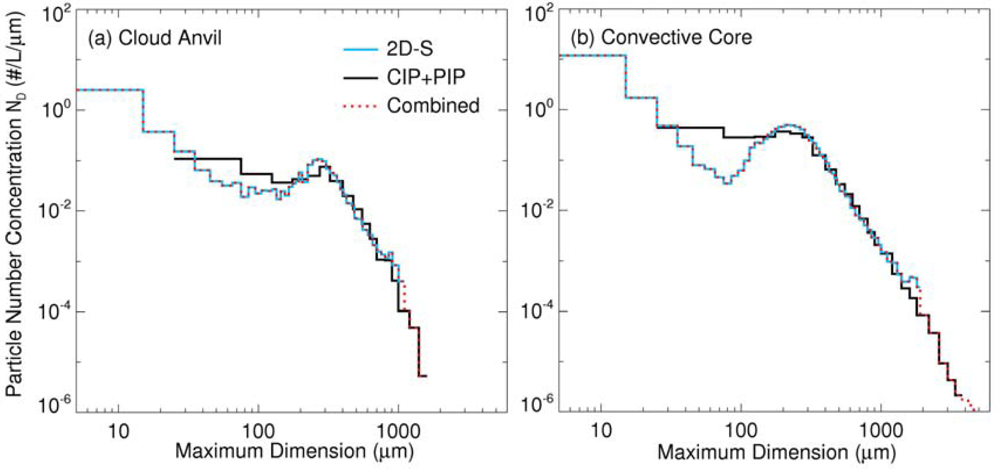
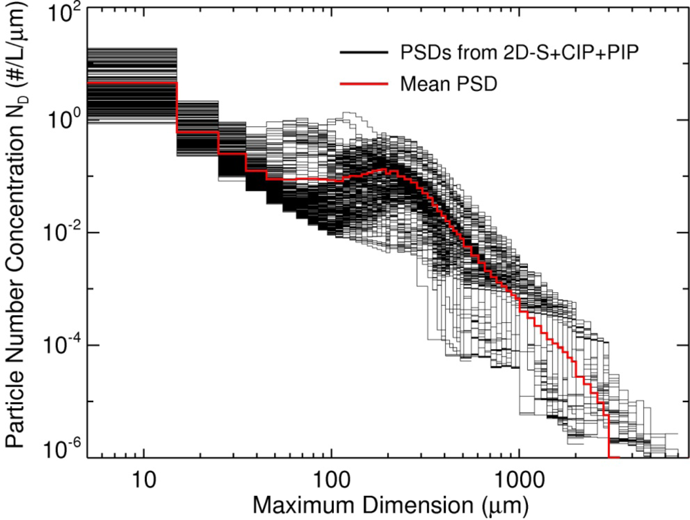
3.3. Cloud Bulk Scattering Properties during the Flight Track

Cloud bulk scattering properties are commonly used to simulate IR radiances emanating from clouds [51–55]. Ice cloud bulk scattering properties are computed by averaging ice particle single scattering properties (i.e., single scattering albedo, absorption and scattering efficiency, asymmetric factor, and scattering phase function) over ice cloud habit and particle size distributions.

Accurate measurements of ice cloud particle size and habit distributions are crucial for ice cloud bulk scattering properties. In this study, ice cloud particle size distributions from the 2D-S, CIP and PIP measurements are combined to construct the particle size distributions with a minimum size bin of 5–15 μm. To minimize the effects of large-crystal shattering on number densities of small ice particles, the particle size distributions from the 2D-S for small ice particles are combined with those from the CIP and PIP for large ice particles. To be consistent with the CIP and PIP data that have been averaged over 5 s or about 1.0 km horizontal path, the 2D-S data are averaged in the same way.

Figure 9 shows the combined ice particle size distributions over an anvil ice cloud and convective core from the 2D-S, CIP, and PIP measurements along the flight track over the deep convective cloud system (Figure 2). High concentrations of small particles are seen in both the anvil at 13:57:09 UTC (Figure 9(a)) and core at 14:02:07 UTC (Figure 9(b)). And both cloud types have a second peak concentrated at a maximum dimension D of 200–300 μm. All of the ice particle size distributions along the DC-8 flight track (Figure 7(a)) are derived and shown in Figure 10. The averaged particle size distribution is used for computing ice cloud bulk scattering properties. Besides the measured particle size distributions, the Gamma particle size distribution (e.g., [56]) is also used for investigating the effects of D_e on the IR radiances from this cloud. The Gamma particle size distribution varies with its parameters, dispersion μ and slope κ. Those used by Hong [56] are adopted here as

$$n(D)=N_0{D}^2\text{exp}\left(-4.87D/D_0\right)$$

(3)

where N₀ is the intercept and D₀ is the median of the distribution.

Also taken from the DC-8, the CPI data were used to resolve the ice cloud particle habits simultaneously with ice particle size distributions during TC⁴. Using an automatic crystal habit classification program, ice particle shapes measured by the CPI were placed into categories including sphere, column, plate, rosette, budding rosette, and irregular for ice particles with D < 50 μm and >50 μm. Figure 11 shows the ice particle habits detected by the CPI along the flight track. It was found that spherical and irregular particles comprise almost all of the habits when D < 50 μm, while the particles with irregular and column habits are most common when D > 50 μm. The averaged habit mixing ratios along the flight track are used for computing ice cloud bulk scattering properties. When D < 50 μm, the habit distribution consists of 55% spheres, 37% irregular particles, and 8% columns. When D > 50 μm, the habit distribution consists of 73% irregular particles, 19% columns, 6% rosettes including rosettes and budding rosettes, 1% spheres, and 1% plates. Single-scattering properties of ice particles with various habits including column, hollow, bullet rosette, plate, aggregate, and droxtal have been investigated extensively (e.g., [53,55,57] and references therein). The single-scattering properties of droxtal, column, plate, rosette, and aggregate particles are used respectively for the sphere, column, plate, rosette, and irregular habits determined from the CPI data.

Following Yang et al., the single-scattering properties of ice particles are then averaged over the habit distributions and particle size distributions to obtain ice cloud bulk scattering properties, which are functions of wavelength, and D_e, which is defined by:

$$D_e=\frac{3}{2}\frac{{\int }_{D_{\text{min}}}^{D_{\text{max}}}\left[\sum _{i=1}^N{f}_i(D)V_i(D)\right]n(D)\text{d}D}{\left[\sum _{i=1}^N{f}_i(D)A_i(D)\right]n(D)\text{d}D}$$

(4)

where f(D) is the particle habit distribution and the summation of f(D) over N equals 1.0, i is the index for N ice particle habits at D, and V and A are the particle volume and projected area, respectively [53]. The liquid cloud is assumed to be composed of spherical water droplets. An effective radius r_e of 10 μm with a gamma particle size distribution following Mishchenko and Travis [50] is used for the water cloud bulk scattering properties. For mixed-phase cloud portions (Figure 8(a)), a water-phase mixing ratio γ is defined by LWC/(IWC + LWC) first, then the bulk scattering properties of mixed-phase clouds are derived by combining those of the ice and water clouds [58–61].

3.4. Effects of Optical Thickness and Particle Size on IR Radiances over Deep Convective Cloud

Simulations and observations of the brightness temperatures at 3.7, 6.7, 7.3, 8.5, 10.8, and 12.0 μm (BT₀₃, BT₀₆, BT₀₇, BT₀₈, BT₁₁, and BT₁₂) over the cloud system are compared to examine the effects of τ and D_e on the IR brightness temperatures.

The correlated k-distribution routines developed by Kratz [62] and Kratz and Rose [63] for the MODIS bands are used to compute the absorption optical depth for each layer in a clear-sky atmosphere. The atmospheric profiles of temperature and humidity (Figure 3), as well as ozone, are used in the correlated k-distribution calculations for each band. The surface emissivity is assumed to be 1.00 for the IR bands. The spectral brightness temperatures over the clouds are then computed with the discrete ordinates radiative transfer model [64] using the constructed cloud τ profiles (Section 3.2), the computed bulk scattering properties, and various D_e in the range of 10–150 μm.

Figure 12 shows the simulated and observed BT values over the subject cloud system as a function of ice cloud τ using the profile in Figure 3(b). Results are similar for most channels. Differences are discussed in Section 4. The mean particle size distribution (D_e = 95 μm) along the flight track is used for the simulations. Since the measured BT₀₃ values include reflected solar radiation while the simulations only include the emitted radiance, the measurements of BT₀₃ are omitted in Figure 12(a). The other simulated values generally agree with the corresponding observations. In particular, for optically thick ice clouds with τ > 20, the simulated values are essentially the same as the observations. For optically thin ice clouds (τ < 1), the simulated BT₀₈, BT₁₁, and BT₁₂ are greater than the observations, while the simulated BT₀₆, BT₀₇, BT₀₈, BT₁₁, and BT₁₂ are less than the observations for ice clouds having 5 < τ < 10 (anvil clouds). These differences are most likely due to the uncertainties in derived ice cloud τ from the CRS (or/and CPL), which can be distinctly different because of the uncertainties in Z_e−LWC relationship [44,65]. The underlying water clouds tend to decrease the BT₀₃, BT₀₈, BT₁₁, and BT₁₂ values for non-opaque ice clouds, but have negligible effect on the water vapor channels’ brightness temperatures. The simulations and observations both reveal that all six BTs are sensitive to ice cloud optical depth for τ up to 20. Furthermore, these sensitivities are essentially monotonic, i.e., these brightness temperatures monotonically decrease with increasing ice cloud optical thickness up to τ = 20. When τ is above 20, the brightness temperatures vary widely although a weak decreasing trend with increasing ice cloud τ is apparent.

The sensitivity of the radiances to phase transition temperature is illustrated in Figure 13, where the 3.7 and 6.7-μm simulations used the −20 °C transition temperature (red) and 0° transition (blue, same as blue in Figure 12). The results are similar for the other channels (not shown). Negligible change is seen in the radiances, but the entire set of radiances is shifted to the right. Thus, the simulated radiances correspond to greater optical depths if it is assumed that the hydrometeors are entirely in the ice phase for T < 0°, as indicated by the in situ data rather than assuming that the layer between 0° and −20 °C is a mixture of ice and water as formulated in Section 3.2 above. This result is encouraging because the phase of clouds in that temperature range is often uncertain.

Figure 14 shows the simulated and observed BTDs among the 3.7, 6.7, 7.3, 8.5, 10.8, and 12.0-μm bands over the cloud system as a function of ice cloud τ. As in Figure 12(a), the BTD(3.7–11) (BTD between 6.7 and 10.8-μm bands and others are similarly defined) measurements are not shown in Figure 14(a). In general, the simulated values of BTD(6.7–11), BTD(8.5–11), BTD(11–12), and BTD(6.7–7.3) are consistent with their respective observations. They are differentially impacted by the presence of low clouds when the ice clouds are optically thin. The water vapor bands at 6.7 and 7.3 μm are affected by upper and middle tropospheric water vapor and above, respectively when the ice clouds are optically thin. This is clearly shown in Figure 14(f), which shows that the simulated BTD(6.7–7.3) values differ significantly from the observations when τ < 3, but dramatically decrease as τ increases. Both the simulated and observed BTDs show strong sensitivities to τ of up to 10. Weak sensitivities to τ up to 20 are also found for BTD(3.7–11), BTD(6.7–11), BTD(3.7–6.7) and BTD(6.7–7.3).

Brightness temperatures for the six bands and their BTDs are commonly used to estimate ice cloud D_e. As noted earlier, previous studies of infrared cloud retrievals have been limited mainly to non-opaque ice clouds having τ < ∼5. Here, the effects of ice particle size D_e on the BTDs and the potential of estimating D_e for optically thick ice clouds are investigated by performing simulations with D_e in the range of 10–150 μm. Figure 15 shows simulated BTDs for various 3.7, 6.7, 7.3, 8.5, 10.8, and 12.0-μm pairs over the subject cloud system as functions of τ and D_e. For these simulations, only ice clouds are involved. The observed BTDs, except for those for the 3.7-μm band with its reflected solar radiances, are also shown together with these simulations. Consistent with previous studies, BTD(3.7–11), BTD(8.5–11), BTD(11–12), and BTD(3.7–6.7) show strong sensitivity to ice cloud D_e when the ice clouds are non-opaque [10,14,19,66]. With τ increasing above ∼3, the differences in BTD(3.7–11), BTD(8.5–11), BTD(11–12), and BTD(3.7–6.7) as a function of D_e decrease eventually. BTD(6.7–11) is essentially insensitive to D_e, which indicates that it could provide a good estimation of τ, since it increases asymptotically toward zero at τ > 20 in the present simulations. BTD(6.7–7.3) only shows differences for D_e < 30 μm. When the opaque ice cloud τ increases, the sensitivity of these BTDs to D_e decreases dramatically. BTD(8.5–11) and BTD(11–12) are only sensitive to small D_e while BTD(3.7–11) and BTD(3.7–6.7) still show weak sensitivity to large values of D_e.

Although BTD(3.7–11), BTD(8.5–11), BTD(11–12), and BTD(3.7–6.7) show significant variability over the deep convective clouds (τ > 20), the general feature of decreasing BTDs with increasing D_e is still apparent. In order to investigate the potential for estimating D_e, the BTDs for each D_e are averaged for ice clouds having τ in the range of 20–100. Figure 16 shows the BTD(3.7–11), BTD(8.5–11), BTD(11–12), and BTD(3.7–6.7) over the tropical deep convective clouds (20 < τ < 100) as a function of D_e. It is evident that BTD(3.7–11) and BTD(3.7–6.7) are sensitive to D_e, especially for D_e > 50. BTD(8.5–11) is only sensitive to D_e values smaller than 50–70 μm and BTD(11–12) is only sensitive to the smallest D_e values. This feature reveals the potential for estimating small D_e using those two BTDs for tropical deep convective clouds during nighttime. The dependencies of BTD(3.7–11) and BTD(3.7–6.7) are likely too small to be useful for a retrieval of D_e for τ > 20 for two reasons. At the low temperatures associated with these thick clouds, the noise at ∼3.7 μm can be as high as 3.5 K [67] and the uncertainty in the water vapor in and around the cloud top can cause errors of ∼1 K (shown later), which cover the range of the signal in Figure 16.

4. Discussion

Simulations of cloud radiance fields necessarily require many assumptions about the cloud, humidity, and temperature horizontal and vertical variations. Differences between the observations and simulations in Figure 14(b,f) are likely due to those assumptions. As noted above, the differences for τ < 6 are probably due to the presence of low or midlevel clouds below thin cirrus clouds. For larger optical depths computed from the CPL and CRS data, the observed water vapor channel BTDs do not appear to reach a distinct asymptote around τ = 8 as seen in the simulations. Rather, the asymptote is not reached until τ = 20 or so. Thus, the vertical variations in D_e, IWC, temperature, and humidity are likely different than assumed and/or higher layer resolution is needed in the calculations. Given the complexities in the actual structure, however, the results are remarkably similar overall.

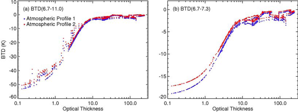
4.1. Sensitivity of BTDs to Uncertainties in Atmospheric Profiles

Nevertheless, it is important to understand how errors in the atmospheric profiles affect the modeled BTDs. The results in Figures 12–15 were all based on the sounding in Figure 3(b), which was considerably moister in the upper troposphere than the profile in Figure 3(a). Such differences may be representative of errors in numerical weather analyses where tropical convection may be properly diagnosed, but offset spatially from where it is actually occurring. To determine how the temperature and moisture profiles affect the radiances, the calculations were performed using the composite smooth sounding in Figure 3(a). The differences in BT and BTD for the two sets of calculations are very small, except for the water vapor channels and their BTDs. Figure 17 shows results for two water vapor channel pairs computed using the two profiles in Figure 3. In all cases, BTD(6.7–11) and BTD(6.7–7.3) are greater using the moister Alajuela sounding. The discrepancies in the BTDs due to the profile difference are mostly between 0.5 and 1 K for τ > 10.

To gain further insight into the sensitivity of the radiances to such errors, four different experiments were conducted. The BTDs of interest were recomputed by systematically varying the upper tropospheric humidity (UTH), the upper tropospheric temperature profile, the cloud top height, and the ice water content profile for the observed cloud system. Results for BTD(3.7–11), BTD(8.5–11), and BTD(11–12) show negligible changes for the scaling in each case. The results for BTD(3.7–6.7) are comparable to those for BTD(6.7–11). Thus, only BTD(6.7–11) and BTD(6.7–7.3) are shown.

Figure 18 shows changes in BTD(6.7–11) (left) and BTD(6.7–7.3) (right) due to systematic variations in water vapor (WV) above 7 (top) and 10 km (bottom) along the aircraft flight path. Because the ice cloud optical thickness varies along the track (Figure 7(c)), the changes vary with τ (replotted in Figure 18(d)). Each curve indicates the differences between the BTDs computed using the nominal relative humidity scaled by 0.5, 0.75, 1.25, and 1.5 and those computed using the nominal humidity profile in Figure 3(b). Decreasing (increasing) the UTH increases (lowers) the BTDs for both spectral pairs. The impact is greatest for thin clouds, particularly for BTD(6.7–11). For clouds having τ > 10, the change in BTD < 1 K, unless a thin cloud lay above the thicker cloud. Overestimation of the UTH for the thin clouds can help explain why the BTDs in Figure 14(b,f) are low relative to the observations. Obviously, the vertical profile of humidity will be considerably different in a column completely filled with clouds than one having clouds in only one layer of the column, so UTH errors of 50% or greater in the vicinity of a cumulonimbus would not be surprising. The impact of the humidity on the BTDs for other band pairs was negligible, except for BTD(3.7–6.7), which yielded results similar, though reversed in sign, to those for BTD(6.7–11).

Similar scaling was applied to the IWC above 10 and 12 km and used to compute the BTDs. Changing the IWC effectively alters the optical thickness of the cloud layer, so it should have a significant impact on thin clouds. Figure 19 presents the results for BTD(6.7–11) and BTD(6.7–7.3). The impact is less than 1.1 K for τ > 20 and smaller than 2 K for 10 < τ < 20. For those cases, an error in IWC of 100% is needed to raise the difference above 1 K. For τ < 10, halving the IWC drops the BTD(6.7–11) by as much as 15 K, while doubling it increases the BTD by as much as (Figure 19(a)). The impacts are much smaller when only part of the cloud is altered (Figure 19(c)) and for BTD(6.7–7.3) as seen in Figure 19(b,d). Biases in the IWC profile could also contribute to the relatively large differences between the computed and observed BTDs seen in Figure 14(b,f). For optically thick clouds, the variation in IWC had an impact less than 0.1 K on BTD(11–12) (not shown). BTD(3.7–6.7) changes due to the IWC variations were slightly larger than those for BTD(6.7–11).

Altering the temperature profiles between 10 and 15 km and between 12 and 15 km by 2 or 4 K produced changes in BTD(6.7–11) and BTD(6.7–7.3) of less than 0.4 K for 10 < τ < 20 and less than 0.2 K for τ > 20 (not shown). Moving the cloud higher by as much as 3 km produced an increase in both BTD(6.7–11) and BTD(6.7–7.3) with values ranging from 0 K for optically thin clouds to increases of up to 4 K for 5 < τ < 20 and down again to ∼ 1 K for τ > 20 (not shown). The increase in BTD(6.7–11) is consistent with a stratospheric penetration by convective clouds [68]. Lowering the cloud by 3 km decreases the thick cloud (τ > 20) 6.7-μm BTDs by as much as 6 K and by up to 15 K for mid-range optical depths. This decrease results from increased WV above the cloud.

The sensitivities illustrated above contribute to uncertainties in the radiance calculations relative to the observations, particularly for the unsampled portions of the cloud contributing to the observed radiances. Differences between the various sensor fields of view also introduce some variability in the observed radiances relative to the calculations. For the most part, it appears that variations in D_e near cloud top could explain much of the thick cloud BTD variability in Figure 15(c,d), but not for the water vapor channel BTDs in Figure 15(b,f). For those channel pairs, a combination of sensor calibration errors, sensor viewing angle differences, and uncertainties in the input data are likely to be responsible for 1–2 K variability in the observations that is not seen in the calculations.

The above results suggest that there is useful information about thick ice cloud optical depth in the BTDs between several channels commonly found on operational meteorological satellites. In particular, the 6.7-μm water vapor channel, when differenced with the 11-μm channel, appears to be most sensitive to τ. The sensitivities to errors in the soundings, cloud temperature, and IWC studied here are typically on the order of 1 K for optically thick clouds. Thus, while the sensitivities of BTD(6.7–11) to changes in thick ice cloud τ indicate that methods to retrieve τ at night can be developed, their results will likely be subject to uncertainties greater than those encountered using solar reflectance methods.

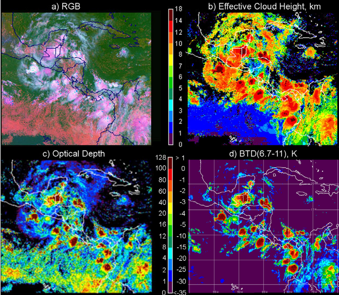
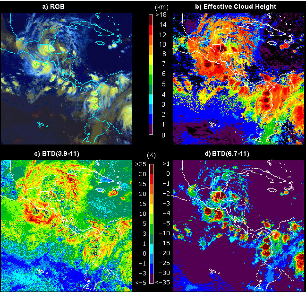
4.2. Satellite Examples of τ Dependency on BTD(6.7–11)

While it is beyond the scope of this paper to completely evaluate the typicality of the above results, it is useful to determine if the dependencies seen here are, at least, qualitatively evident in satellite imagery. Figure 20 shows imagery over Central America from GOES-12 taken at the same time as the example presented above. The pseudocolor RGB (red: BT₁₁, scale reversed; green: BTD(3.9–11); and blue: 0.65-μm reflectance) and BTD(6.7–11) images are shown in Figures 20a and 20d, respectively. Figure 20(b,c) depicts the effective cloud height Z_c and τ, respectively, derived using the methods of Minnis et al. [10]. Generally, in these images, wherever Z_c > 6 km and τ > 4, BTD(6.7–11) > −20 K or so. While there is not perfect correlation, some of the large optical depths are caused by thin cirrus over thick stratus, it is clear that the gradients in BTD(6.7–11) correspond, to some extent, to the gradients in τ for the thicker portions of the high clouds.

At night, similar gradients in BTD(6.7–11) are evident around the convective cells in the 1045 UTC GOES-12 imagery for 5 August 2007 (Figure 21). The correspondence between the highest clouds and the BTD(6.7–11) gradients around the cores is as strong in Figure 21(b,d) as those seen in Figure 20, suggesting similar variations in τ. The imagery also highlights some of the difficulties that will be encountered when trying to use such spectral signals to retrieve τ. The midlevel (5–7 km in Figure 21(b)) clouds over the Andes and even some of the marine stratus clouds in the lower left part of the image are also accompanied by some variations in BTD(6.7–11) that approach −20 K. With even drier atmospheres over mid- and lower-level clouds in other areas, BTD(6.7–11) will be even closer to 0 K. Thus, other information such as cloud height (e.g., Figure 21(b)) and other channel BTDs, as well as accurate temperature and water vapor profiles would be needed to unravel the BTD(6.7–11) signal.

There are considerable variations in BTD(3.9–11) in Figure 21(c) with the largest values (>30 K) occurring in the anvil-generated cirrus. The 3.7 and 3.9-μm channels are similar enough to make some inferences from Figure 15(a). The greatest values likely correspond to smaller values of D_e for 2 < τ < 8.

As the optical depth increases toward the core, BTD(3.9–11) drops precipitously to <10 K and eventually becomes noisy over the core because the accuracy of BT₀₃ is greatly diminished at the lowest temperatures (<205 K). The gradient in BTD(3.7–11) over a convective core can be seen more clearly for the developing storms just southwest of Hispaniola. There, BTD(6.7–11) is close to −1 K, which would correspond to 30 < τ < 100 (Figure 15(b)) and the smallest value of BTD(3.7–11) is ∼5 K, which would correspond to small particles at the cloud top (Figure 21(b)). While the earlier discussion regarding the small gradient in BTD(3.7–11) with increasing D_e would be overwhelmed by noise in the detector at low temperatures, the satellite observations suggest that D_e could be retrieved at night for many of the thicker ice clouds, but not for the coldest clouds. More likely, such a retrieval would be limited to clouds with τ < 20. Further research is needed to clarify the range of optical depths and temperatures for which such retrievals would be useful.

The case presented in the previous section used a tropical convective system and may have characteristics unlike high clouds in mid-latitudes and polar regions. Figure 22 shows imagery from the Meteosat-9 Spinning Enhanced Visible Infrared Imager (SEVIRI) taken at 1200 UTC, 1 June 2012 over Europe. The RGB image (Figure 22(a)) shows baroclinic systems over the eastern and western sides of the domain with stratus clouds between and cirrus clouds over Italy and North Africa. Cloud optical depths retrieved with the methods of Minnis et al. [10] exceed 100 over parts of the eastern system and are greater than 20–40 over portions of the western high clouds. Although the correspondence of BTD(6.7–11) in Figure 22(c) with τ is less obvious than seen in Figure 20, some is still present. This diminished correspondence could be due to the considerable amount of multi-layered clouds occurring in the baroclinic systems and the higher viewing zenith angles for the domain. The variations in τ derived using the 0.65-μm reflectance are due to the total column cloud optical depth, while τ for the upper layer clouds should primarily be responsible for variations in BTD(6.7–11). While this difference in sensitivity could raise some obstacles to retrieving τ at night, it could also provide a means for detecting multilayered clouds and, perhaps, retrieving their properties using an approach similar to that of Chang et al. [69].

The information in the BTD(8.5–11) and BTD(11–12) images in Figure 22(d) and 22(e), respectively, could also aid in the determination of multilayered cloud conditions and the utility of the BTD(6.7–11) for thick cloud τ retrievals. For example, the large values of BTD(8.5–11) and BTD(11–12) over Italy and North Africa indicate that the high clouds have τ < ∼4 and small values of D_e. The near-zero values for both channel differences over much of the frontal cloudiness suggest that the ice clouds are opaque and the retrieval of τ using BTD(6.7–11) would apply only to ice clouds. If it is significantly different from the visible channel τ retrieval, then it could be concluded that a multilayered or contiguous, very thick cloud was present. Figure 22(f) shows the results of applying the 11 and 13.4-μm channel method of Chang et al. to the same image [69]. Most of the clouds classified as thick multilayer or thick high clouds by the Chang et al. technique correspond to areas where BTD(6.7–11) > −15 K [69]. Thus, it appears that even in the absence of the 13.4-μm channel, it may be possible to obtain valuable multilayered cloud information using the 6.7 and 11-μm channels common to all current and most older geostationary satellites.

5. Conclusions

With the aid of TC⁴ aircraft measurements of radiances over a tropical deep convective cloud system and simulations of radiances using in situ measurements of cloud properties, this paper has investigated the sensitivities of brightness temperatures for these bands and their differences to ice cloud τ and D_e. Measurements from two aircraft and surface-based radiosondes were used in a detailed radiative transfer model to simulate radiances at various MODIS channels that would emanate from a deep convective cloud complex. The simulated radiances were compared with radiance measurements taken at nadir from two instruments on the ER-2 and adjusted to the MODIS filter functions.

The simulated BTs are generally consistent with the corresponding observations, particularly, for optically thick ice clouds with τ > 20 (i.e., deep convective clouds). The IR radiances emitted from deep convective clouds are essentially the result of contributions from the cloud and from atmospheric gaseous absorption and emission above the clouds (upper troposphere), which can be neglected for the window bands, 3.7, 8.5, 10.8 and 12.0 μm. Both the simulations and observations of these IR brightness temperatures monotonically decrease with increasing ice cloud τ up to ∼20. Although, in some instances, significant differences are found between the absolute values of the simulations and observations, a weak decreasing trend is found with increasing ice cloud τ when τ is above 20. Similar to the brightness temperature comparisons, simulated BTDs among these bands generally agree with the observations within the range of uncertainties in the input data. Both simulated and observed BTD(3.7–11), BTD(6.7–11), BTD(3.7–6.7), and BTD(6.7–7.3) are sensitive to ice cloud τ up to ∼20. This dependency is accompanied by uncertainties due to sensitivities of the BTDs to errors in the atmospheric profiles of temperature, humidity, ice water content, and cloud top height that can be as large or larger than the variation of BTD with τ.

The sensitivity of BTDs to D_e was also investigated. BTD(6.7–11) has no sensitivity to D_e. This feature provides an advantage for estimating ice cloud τ. Consistent with previous studies on estimating ice cloud D_e using IR BTDs, BTD(3.7–11), BTD(8.5–11), BTD(11–12), and BTD(3.7–6.7) show strong sensitivity to D_e of non-opaque ice clouds. With increasing ice cloud τ, the sensitivity weakens. Over deep convective clouds (τ > 20), both BTD(3.7–11) and BTD(3.7–6.7) show sensitivity to D_e while BTD(8.5–11) is only sensitive to small D_e that are less than 50–70 μm and BTD(11–12) is sensitive to even smaller D_e. Unfortunately, the D_e signal is likely to be overwhelmed by the noise in some channels at cold temperatures and uncertainties in the vertical profiles of temperature, humidity, and ice water content. Additional research is needed to define the range of temperatures and optical depths for which D_e could be retrieved using the spectral bands considered here.

The simulated results are also generally consistent with satellite observations taken at similar wavelengths and indicate that some combination of these channels, particularly the 3.7, 6.7, and 11-μm channels, could be used for retrieving the optical depths of ice clouds that exceed the typical opaque limit of 6 for cloud optical depth. While many challenges and obstacles, such as the size of the uncertainties in input data, would need to be overcome, it may be possible to use such information to provide better quantitative monitoring of ice clouds over the entire diurnal cycle. Such a capability would aid both climate and weather studies because clouds are an essential component of the radiation and water budgets of the atmosphere both day and night.

References and Notes

- Liou, K.-N. Influence of cirrus clouds on weather and climate processes: A global perspective. Mon. Wea. Rev 1986, 114, 1167–1199. [Google Scholar]
- Ramanathan, V.; Collins, W. Thermodynamic regulation of ocean warming by cirrus clouds deduced from observations of the 1987 El Niño. Nature 1991, 351, 27–32. [Google Scholar]
- Zhang, M.H.; Lin, W.Y.; Klein, S.A.; Bacmeister, J.T.; Bony, S.; Cederwall, R.T.; Del Genio, A.D.; Hack, J.J.; Loeb, N.G.; Lohmann, U.; et al. Comparing clouds and their seasonal variations in 10 atmospheric general circulation models with satellite measurements. J. Geophys. Res 2005, 110. [Google Scholar] [CrossRef]
- Rossow, W.B.; Schiffer, R.A. Advances in understanding clouds from ISCCP. Bull. Amer. Meteor. Soc 1999, 80, 2261–2288. [Google Scholar]
- Wylie, D.P.; Jackson, D.L.; Menzel, W.P.; Bates, J.J. Trends in global cloud cover in two decades of HIRS observations. J. Climate 2005, 18, 3021–3031. [Google Scholar]
- Jones, T.A.; Stensrud, D.J.; Minnis, P.; Palikonda, R. Evaluation of a forward operator to assimilate cloud water path into WRF-DART. Mon. Wea. Rev 2012. submitted. [Google Scholar]
- Norris, P.M.; da Silva, A.M. Monte Carlo Bayesian inference on a statistical model of sub-grid column moisture variability using high-resolution cloud observations. Part I: Sensitivity tests and results. Q. J. R. Meteorol. Soc 2012. submitted. [Google Scholar]
- King, M.D.; Menzel, P.; Kaufman, Y.J.; Tanre, D.; Gao, B.-C.; Platnick, S.; Ackerman, S.A.; Remer, L.A.; Pincus, R.; Hubanks, P.A. Cloud and aerosol properties, precipitable water, and profiles of temperature and water vapor from MODIS. IEEE Trans. Geosci. Remote Sens 2003, 41, 442–458. [Google Scholar]
- Minnis, P.; Takano, Y.; Liou, K.-N. Inference of cirrus cloud properties using satellite-observed visible and infrared radiances, Part I: Parameterization of radiance fields. J. Atmos. Sci 1993, 50, 1279–1304. [Google Scholar]
- Minnis, P.; Szedung, S.-M.; Young, D.F.; Heck, P.W.; Garber, D.P.; Chen, Y.; Spangenberg, D.A.; Arduini, R.F.; Trepte, Q.Z.; Smith, W.L.; et al. CERES Edition-2 cloud property retrievals using TRMM VIRS and Terra and Aqua MODIS data, Part I: Algorithms. IEEE Trans. Geosci. Remote Sens 2011, 49, 4374–4400. [Google Scholar]
- Platnick, S.; King, M.D.; Ackerman, S.A.; Menzel, W.P.; Baum, B.A.; Riédi, J.C.; Frey, R.A. The MODIS cloud products: Algorithms and examples from Terra. IEEE Trans. Geosci. Remote Sens 2003, 41, 459–473. [Google Scholar]
- Heidinger, A.K. Rapid daytime estimation of cloud properties over a large area from radiance distributions. J. Atmos. Ocean. Tech 2003, 20, 1237–1250. [Google Scholar]
- Hong, G.; Minnis, P.; Doelling, D.R.; Ayers, J.K.; Sun-Mack, S. Estimating effective particle size of tropical deep convective clouds with a look-up table method using satellite measurements of brightness temperature differences. J. Geophys. Res 2012, 117. [Google Scholar] [CrossRef]
- Wu, M.C. A method for remote sensing the emissivity, fractional cloud cover, and cloud top temperature of high-level, thin clouds. J. Climate Appl. Meteor 1987, 26, 225–233. [Google Scholar]
- Menzel, W.P.; Richard, F.; Zhang, H.; Wylie, D.P.; Moeller, C.; Holz, R.E.; Maddux, B.; Strabala, K.I.; Gumley, L.E. MODIS global cloud-top pressure and amount estimation: Algorithm description and results. J. Appl. Meteorol. Climatol 2008, 47, 1175–1198. [Google Scholar]
- Inoue, T. On the temperature and effective emissivity determination of semi-transparent cirrus clouds by bispectral measurements in the 10 micron window region. J. Meteor. Soc. Japan 1985, 63, 88–99. [Google Scholar]
- Hong, G.; Yang, P.; Heidinger, A.K.; Pavolonis, M.J.; Baum, B.A.; Platnick, S.E. Detecting opaque and nonopaque tropical upper tropospheric ice clouds: A trispectral technique based on the MODIS 8–12 μm window bands. J. Geophys. Res 2010, 115. [Google Scholar] [CrossRef]
- Lin, X.; Coakley, J., Jr. Retrieval of properties for semitransparent clouds from multispectral infrared imagery data. J. Geophys. Res 1993, 98, 18501–18514. [Google Scholar]
- Ou, S.C.; Liou, K.-N.; Gooch, W.M.; Takano, Y. Remote sensing of cirrus cloud properties using Advanced Very-High Resolution Radiometer 3.7 and 10.9-μm channels. Appl. Opt 1993, 32, 2171–2180. [Google Scholar]
- Szejwach, G. Determination of semitransparent cirrus cloud temperature from infrared radiances: Application to METEOSAT. J. Appl. Meteor 1982, 21, 384–393. [Google Scholar]
- Liou, K.-N.; Ou, S.C.; Takano, Y.; Valero, F.P.J.; Ackerman, T.P. Remote sounding of the tropical cirrus cloud temperature and optical depth using 6.5 and 10.5 μm radiometers during STEP. J. Appl. Meteor 1990, 29, 716–726. [Google Scholar]
- Huang, H.-L.; Yang, P.; Wei, H.; Baum, B.A.; Hu, Y.X.; Atonelli, P.; Ackerman, S.A. Inference of ice cloud properties from high spectral resolution infrared observations. IEEE Trans. Geosci. Remote Sens 2004, 42, 842–852. [Google Scholar]
- Kahn, B.H.; Eldering, A.; Ghil, M.; Bordoni, S.; Clough, S.A. Sensitivity analysis of cirrus cloud properties from high resolution infrared spectra, Part I: Methodology and synthetic cirrus. J. Climate 2004, 17, 4856–4870. [Google Scholar]
- Yue, Q.; Liou, K.-N. Cirrus cloud optical and microphysical properties determined from AIRS infrared spectra. Geophys. Res. Lett 2009, 36, L05810. [Google Scholar] [CrossRef]
- Chaboureau, J.-P.; Bechtold, P. Statistical representation of clouds in a regional model and the impact on the diurnal cycle of convection during Tropical Convection, Cirrus and Nitrogen Oxides (TROCCINOX). J. Geophys. Res 2005, 110, D17103. [Google Scholar] [CrossRef]
- Hong, G.; Yang, P.; Gao, B.-C.; Baum, B.A.; Hu, Y.X.; King, M.D.; Platnick, S. High cloud properties from three years of MODIS Terra and Aqua data over the Tropics. J. Appl. Meteor. Climatol 2007, 46, 1840–1856. [Google Scholar]
- Hong, G.; Heygster, G.; Notholt, J.; Buehler, S.A. Interannual to diurnal variations in tropical and subtropical deep convective clouds and convective overshooting from seven years of AMSU-B measurements. J. Climate 2008, 21, 4168–4189. [Google Scholar]
- Bedka, K. M.; Minnis, P. GOES-12 observations of convective storm variability and evolution during the TC4 field program. J. Geophys. Res 2010, 115, D00J13. [Google Scholar] [CrossRef]
- Wood, R. Marine stratocumulus. Mon. Wea. Rev 2012, 140, 2373–2423. [Google Scholar]
- Toon, O.B.; Starr, D.O.; Jensen, E.J.; Newman, P.A.; Platnick, S.; Schoeberl, M.R.; Wennberg, P.O.; Wofsy, S.C.; Kurylo, M.J.; Maring, H.; Jucks, K.W.; et al. Planning, implementation, and first results of the Tropical Composition, Cloud and Climate Coupling Experiment (TC4). J. Geophys. Res 2010, 115. [Google Scholar] [CrossRef]
- Hook, S.J.; Myers, J.J.; Thome, K.J.; Fitzgerald, M.; Kahle, A.B. The MODIS/ASTER airborne simulator (MASTER)—A new instrument for earth science studies. Remote Sens. Environ 2001, 76, 93–102. [Google Scholar]
- King, M.D.; Platnick, S.; Wind, G.; Arnold, G.T.; Dominguez, R.T. Remote sensing of radiative and microphysical properties of clouds during TC4: Results form MAS, MASTER, MODIS, and MISR. J. Geophys. Res 2010, 11, D00J07. [Google Scholar] [CrossRef]
- Revercomb, H.E.; Walden, V.P.; Tobin, D.C.; Anderson, J.; Best, F.A.; Ciganovich, N.C.; Dedecker, R.G.; Dirkx, T.; Ellington, S.C.; Garcia, R.K.; et al. Recent results from two new aircraft-based Fourier transform interferometers: The Scanning High-Resolution Interferometer Sounder and the NPOESS Atmospheric Sounder Testbed Interferometer. Proceedings of 8th International Workshop of Atmospheric Science From Space Using Fourier Transform Spectrometry, Toulouse, France, 16–18 November 1998; pp. 1–6.
- Li, L.; Heymsfield, G.M.; Racette, P.E.; Tian, L.; Zenker, E. A 94 GHz cloud radar system on a NASA high-altitude ER-2 aircraft. J. Atmos. Ocean. Tech 2004, 21, 1378–1388. [Google Scholar]
- McGill, M.J.; Li, L.; Hart, W.D.; Heymsfield, G.M.; Hlavka, D.L.; Racette, P.E.; Tian, L.; Vaughan, M.A.; Winker, D.M. Combined lidar-radar remote sensing: Initial results from CRYSTAL-FACE. J. Geophys. Res 2004, 109, D07203. [Google Scholar] [CrossRef]
- McGill, M.J.; Hlavka, D.L.; Hart, W.D.; Spinhirne, J.D.; Scott, V.S.; Schmid, B. The Cloud Physics Lidar: Instrument description and initial measurement results. Appl. Opt 2002, 41, 3725–3734. [Google Scholar]
- Jensen, E.J.; Lawson, P.; Baker, B.; Pilson, B.; Mo, Q.; Heymsfield, A.J.; Bansemer, A.; Bui, T.P.; McGill, M.; Hlavka, D.; et al. On the importance of small ice crystals in tropical anvil cirrus. Atmos. Chem. Phys 2009, 9, 5321–5370. [Google Scholar]
- Lawson, R.P.; O’Connor, D.; Zmarzly, P.; Weaver, W.; Baker, B.A.; Mo, Q.; Jonsson, H. The 2D-S (Stereo) probe: Design and preliminary tests of a new airborne, high-speed, high-resolution imaging probe. J. Atmos. Ocean. Tech 2006, 23, 1462–1477. [Google Scholar]
- Field, P.R.; Heymsfield, A.J.; Bansemer, A. Shattering and particle interarrival times measured by optical array probes in ice clouds. J. Atmos. Ocean. Tech 2006, 23, 1357–1371. [Google Scholar]
- Baumgardner, D.; Jonsson, H.; Dawson, W.; O’Connor, D.; Newton, R. The cloud, aerosol and precipitation spectrometer (CAPS): A new instrument for cloud investigations. Atmos. Res 2002, 59–60, 251–264. [Google Scholar]
- Heymsfield, A.J.; Bansemer, A.; Schmitt, C.G.; Twohy, C.; Poellet, M.R. Effective ice particle densities derived from aircraft data. J. Atmos. Sci 2004, 61, 982–1003. [Google Scholar]
- Tian, L.; Heymsfield, G.M.; Heymsfield, A.J.; Bansemer, A.; Li, L.; Twohy, C.H.; Srivastava, R.C. A study of cirrus ice particle size distribution using TC4 observations. J. Atmos. Sci 2010, 67, 195–216. [Google Scholar]
- Thompson, A.M.; MacFarlane, A.M.; Morris, G.A.; Yorks, J.E.; Miller, S.K.; Taubman, B.F.; Verver, G.; Vömel, H.; Avery, M.A.; Hair, J.W.; et al. Convective and wave signatures in ozone profiles over the equatorial Americas: Views from TC4 2007 and SHADOZ. J. Geophys. Res 2010, 115, D00J23. [Google Scholar] [CrossRef]
- Minnis, P.; Yost, C.R.; Sun-Mack, S.; Chen, Y. Estimating the physical top altitude of optically thick ice clouds from thermal infrared satellite observations using CALIPSO data. Geophys. Res. Lett 2008, 35, L12801. [Google Scholar] [CrossRef]
- Austin, R.T.; Heymsfield, A.J.; Stephens, G.L. Retrieval of ice cloud microphysical parameters using the CloudSat millimeter-wave radar and temperature. J. Geophys. Res 2009, 114, D00A23. [Google Scholar] [CrossRef]
- Baedi, R.J.P.; de Wit, J.J.M.; Russchenberg, H.W.J.; Erkelens, J.S.; Baptista, J.P.V.P. Estimating effective radius and liquid water content from radar and lidar based on the CLARE98 data set. Phys. Chem. Earth B 2000, 25, 1057–1062. [Google Scholar]
- Liu, C.L.; Illingworth, A.J. Toward more accurate retrievals of ice water content from radar measurements of clouds. J. Appl. Meteorol 2000, 39, 1130–1146. [Google Scholar]
- Marzano, F.S.; Mugnai, A.; Panegrossi, G.; Pierdicca, N.; Smith, E.A.; Turk, J. Bayesian estimation of precipitating cloud parameters from combined measurements of spaceborne microwave radiometer and radar. IEEE Trans. Geosci. Remote Sens 1999, 37, 596–613. [Google Scholar]
- Skofronick-Jackson, G.M.; Wang, J.R.; Heymsfield, G.M.; Hood, R.; Manning, W.; Meneghini, R.; Weiman, J.A. Combined radiometer-radar microphysical profile estimations with emphasis on high-frequency brightness temperature observations. J. Appl. Meteorol 2003, 42, 476–487. [Google Scholar]
- Heymsfield, A.J.; Matrosov, S.; Baum, B. Ice water path–optical depth relationships for cirrus and deep stratiform ice cloud layers. J. Appl. Meteor 2003, 42, 1369–1390. [Google Scholar]
- Mishchenko, M.I.; Travis, L.D. Capabilities and limitations of a current FORTRAN implementation of the T-matrix method for randomly oriented, rotationally symmetric scatterers. J. Quant. Spectrosc. Radiat. Transfer 1998, 60, 309–324. [Google Scholar]
- Baran, A.J. On the scattering and absorption properties of cirrus cloud. J. Quant. Spectrosc. Radiat. Transfer 2004, 89, 17–36. [Google Scholar]
- Baum, B.A.; Heymsfield, A.J.; Yang, P.; Bedka, S.T. Bulk scattering properties for the remote sensing of ice clouds. Part I: Microphysical data and models. J. Appl.Meteor 2005, 44, 1885–1895. [Google Scholar]
- Yang, P.; Wei, H.; Huang, H.-L.; Baum, B.A.; Hu, Y.X.; Kattawar, G.W.; Mishchenko, M.I.; Fu, Q. Scattering and absorption property database for nonspherical ice particles in the near through far-infrared spectral region. Appl. Opt 2005, 44, 5512–5523. [Google Scholar]
- Kokhanovsky, A.A. Light Scattering Reviews 4: Single Light Scattering and Radiative Transfer; Praxis Publishing Ltd.: Chichester, UK, 2009; p. 534. [Google Scholar]
- Kosarev, A.L.; Mazin, I.P. An empirical model of the physical structure of upper layer clouds. Atmos. Res 1999, 26, 213–228. [Google Scholar]
- Hong, G. Parameterization of scattering and absorption properties of nonspherical ice crystals at microwave frequencies. J. Geophys. Res 2007, 112, D11208. [Google Scholar] [CrossRef]
- Baran, A.J. A review of the light scattering properties of cirrus. J. Quant. Spectrosc. Radiat. Transfer 2009, 110, 1239–1260. [Google Scholar]
- Yang, P.; Wei, H.L.; Baum, B.A.; Huang, H.-L.; Heymsfield, A.J.; Hu, Y.X.; Gao, B.-C.; Turner, D.D. The spectral signature of mixed-phase clouds composed of nonspherical ice crystals and spherical liquid droplets in the terrestrial window region. J. Quant. Spectrosc. Radiat. Transf 2003, 79, 1171–1188. [Google Scholar]
- Lee, J.; Yang, P.; Dessler, A.; Baum, B.A.; Platnick, S. The influence of thermodynamic phase on the retrieval of mixed-phase cloud microphysical and optical properties in the visible and near-infrared region. IEEE Geosci. Remote Sens. Lett 2006, 3, 287–291. [Google Scholar]
- Ou, S.C.; Liou, K.N.; Wang, X.J.; Hagan, D.; Dybdahl, A.; Mussetto, M.; Carey, L.D.; Niu, J.; Kankiewicz, J.A.; Kidder, S.; Vonder Haar, T.H. Retrievals of mixed-phase cloud properties during the National Polar-Orbiting Operational Environmental Satellite System. Appl. Opt 2009, 48, 1452–1462. [Google Scholar]
- Mitchell, D.L.; Lawson, R.P.; Baker, B. Understanding effective diameter and its application to terrestrial radiation in ice clouds. Atmos. Chem. Phys 2011, 11, 3417–3429. [Google Scholar]
- Kratz, D.P. The correlated k-distribution technique as applied to the AVHRR channels. J. Quant. Spectrosc. Radiat. Transfer 1995, 53, 501–517. [Google Scholar]
- Kratz, D.P.; Rose, F.G. Accounting for molecular absorption within the spectral range of the CERES window channel. J. Quant. Spectrosc. Radiat. Transfer 1999, 61, 83–95. [Google Scholar]
- Stamnes, K.; Tsay, S.-C.; Wiscombe, W.J.; Jayaweera, K. Numerically stable algorithm for discrete-ordinate-method radiative transfer in multiple scattering and emitting layered media. Appl. Opt 1998, 27, 2502–2509. [Google Scholar]
- Hong, G.; Yang, P.; Baum, B.A.; Heymsfield, A.J. Relationship between ice water content and equivalent radar reflectivity for clouds consisting of nonspherical ice particles. J. Geophys. Res 2008, 113, D20205. [Google Scholar] [CrossRef]
- Minnis, P.; Garber, D.P.; Young, D.F.; Arduini, R.F.; Takano, Y. Parameterization of reflectance and effective emittance for satellite remote sensing of cloud properties. J. Atmos. Sci 1998, 55, 3313–3339. [Google Scholar]
- Menzel, W.P.; Purdom, J.F.W. Introducing GOES-I: The first of a new generation of Geostationary Operational Environmental Satellites. Bull. Amer. Meteor. Soc 1994, 75, 757–781. [Google Scholar]
- Schmetz, J.; Tjemkes, S.A.; Gube, M.; van der Berg, L. Monitoring deep convection and convective overshooting with METEOSAT. Adv. Space Res 1997, 19, 433–441. [Google Scholar]
- Chang, F.-L.; Minnis, P.; Sun-Mack, S.; Kato, S.; Chen, Y. Passive and active remote sensing of multilayer clouds: A look at GOES, MODIS, CALIPSO, CloudSat and ARM SGP observations. J. Atmos. Sci 2012. submitted. [Google Scholar]
Share and Cite
Minnis, P.; Hong, G.; Ayers, J.K.; Smith, W.L., Jr.; Yost, C.R.; Heymsfield, A.J.; Heymsfield, G.M.; Hlavka, D.L.; King, M.D.; Korn, E.; et al. Simulations of Infrared Radiances over a Deep Convective Cloud System Observed during TC4: Potential for Enhancing Nocturnal Ice Cloud Retrievals. Remote Sens. 2012, 4, 3022-3054. https://doi.org/10.3390/rs4103022
Minnis P, Hong G, Ayers JK, Smith WL Jr., Yost CR, Heymsfield AJ, Heymsfield GM, Hlavka DL, King MD, Korn E, et al. Simulations of Infrared Radiances over a Deep Convective Cloud System Observed during TC4: Potential for Enhancing Nocturnal Ice Cloud Retrievals. Remote Sensing. 2012; 4(10):3022-3054. https://doi.org/10.3390/rs4103022
Chicago/Turabian StyleMinnis, Patrick, Gang Hong, J. Kirk Ayers, William L. Smith, Jr., Christopher R. Yost, Andrew J. Heymsfield, Gerald M. Heymsfield, Dennis L. Hlavka, Michael D. King, Errol Korn, and et al. 2012. "Simulations of Infrared Radiances over a Deep Convective Cloud System Observed during TC4: Potential for Enhancing Nocturnal Ice Cloud Retrievals" Remote Sensing 4, no. 10: 3022-3054. https://doi.org/10.3390/rs4103022
APA StyleMinnis, P., Hong, G., Ayers, J. K., Smith, W. L., Jr., Yost, C. R., Heymsfield, A. J., Heymsfield, G. M., Hlavka, D. L., King, M. D., Korn, E., McGill, M. J., Selkirk, H. B., Thompson, A. M., Tian, L., & Yang, P. (2012). Simulations of Infrared Radiances over a Deep Convective Cloud System Observed during TC4: Potential for Enhancing Nocturnal Ice Cloud Retrievals. Remote Sensing, 4(10), 3022-3054. https://doi.org/10.3390/rs4103022