MERIS Retrieval of Water Quality Components in the Turbid Albemarle-Pamlico Sound Estuary, USA


Abstract
:1. Introduction
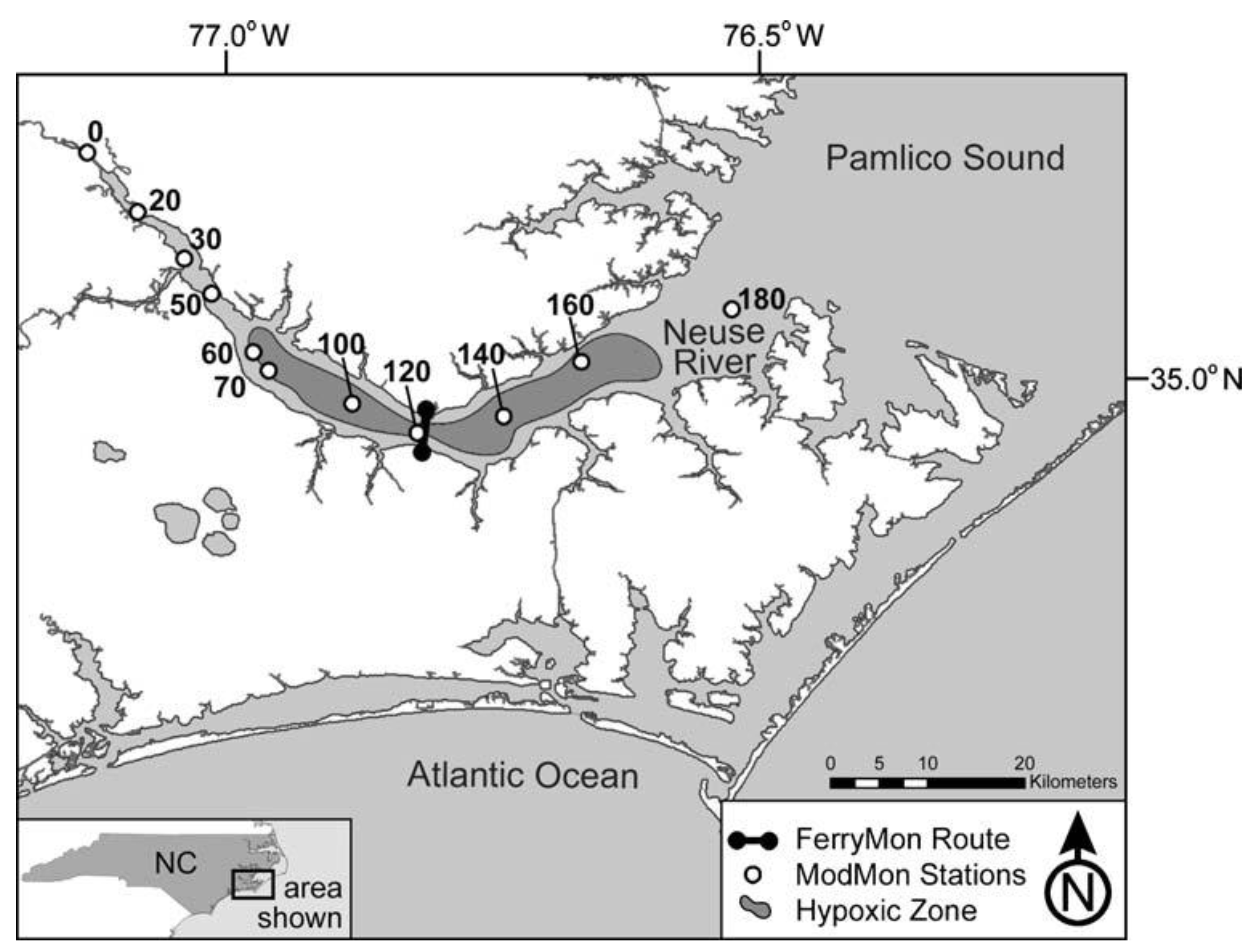
1.1. Study Area
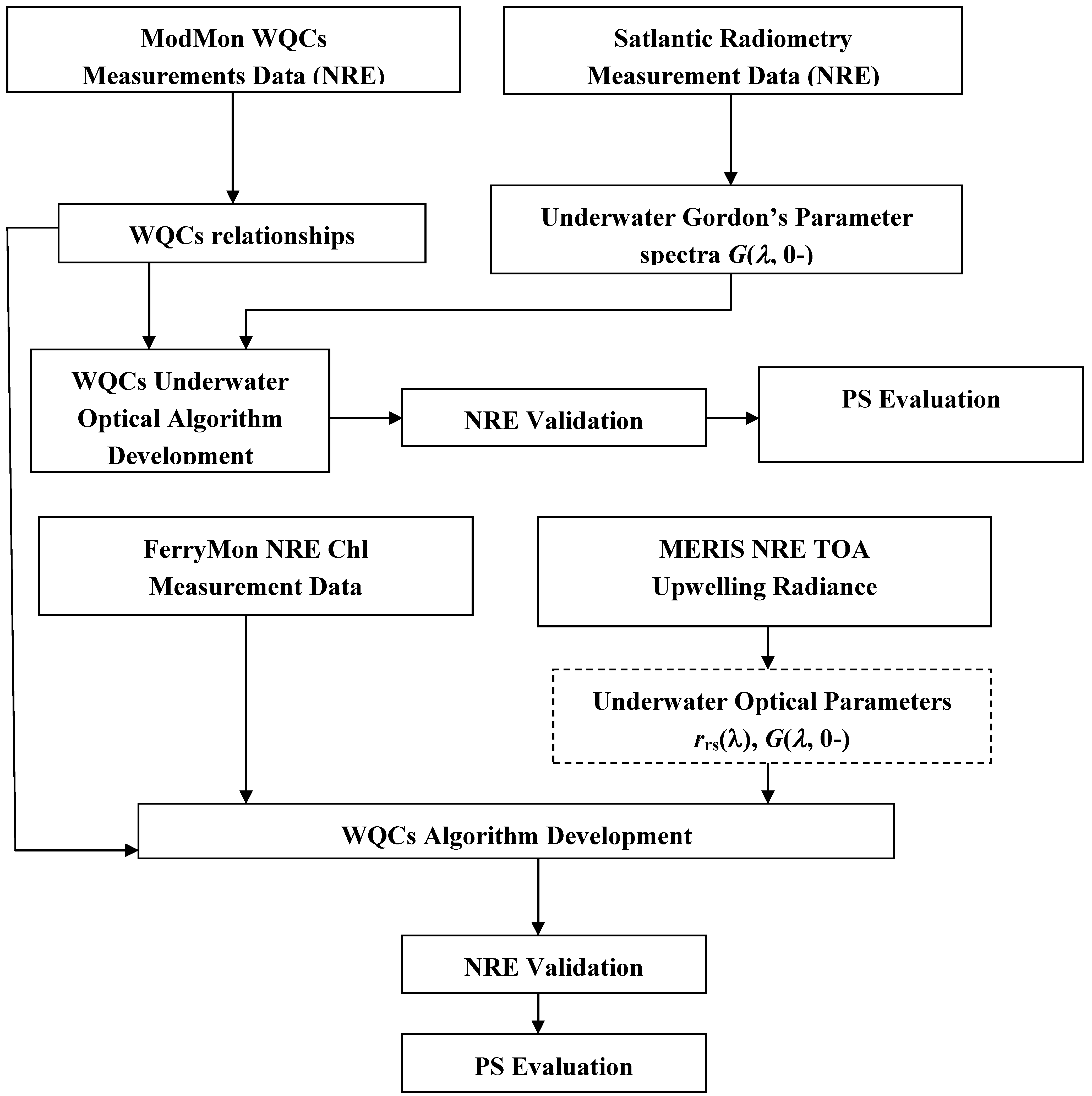
2. Methods
2.1. Radiometric Measurements

2.2. Water Quality Measurements
2.3. Satellite Imagery
2.4. Water Quality Retrieval Algorithms
3. Results and Discussion
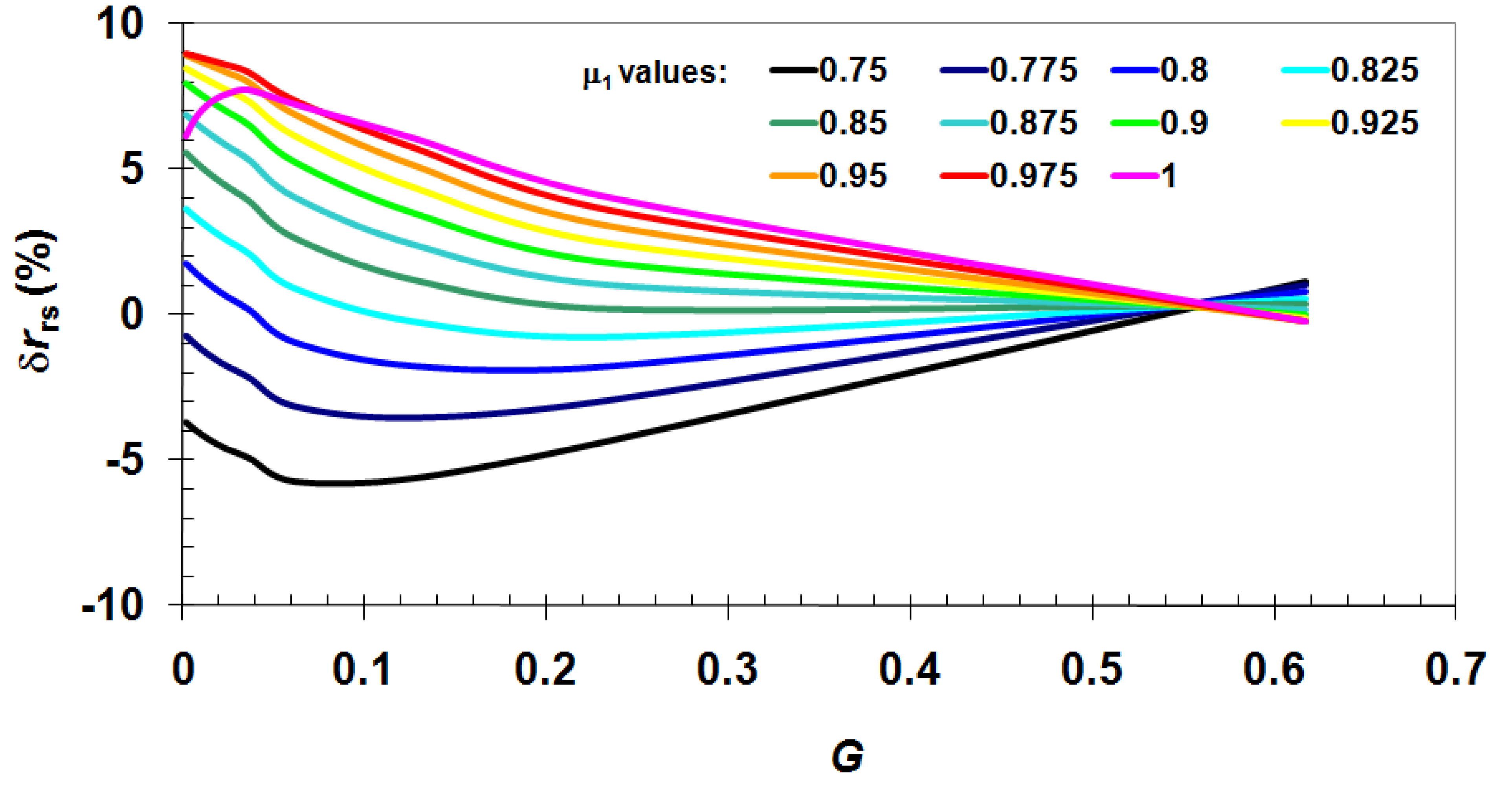
3.1. Validation of rrs Approximations
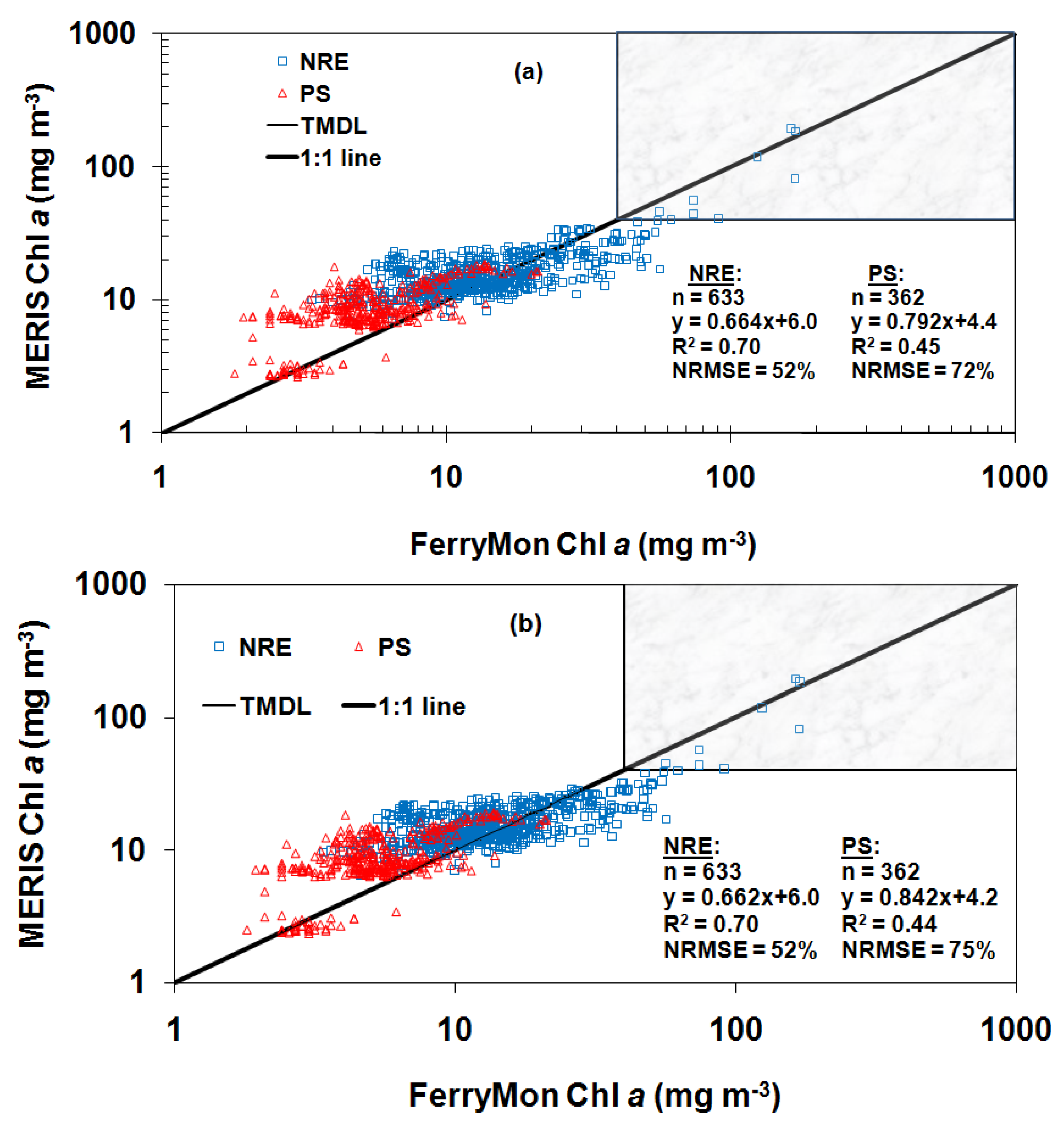
3.2. Validation of WQC Algorithms


| n | Mean (mg m−3) | SD (mg m−3) | CV (%) | NMBE (%) | NRMSE (%) | R2 | p | Intercept (mg m−3) | Slope |
|---|---|---|---|---|---|---|---|---|---|
| Neuse River Estuary | |||||||||
| 633 | 17.7 | 12.6 | 71 | 2.7 | 52 | 0.70 | 3 × 10−165 | 6.0 | 0.66 |
| 633 | 17.8 | 12.4 | 70 | 2.8 | 52 | 0.70 | 6 × 10−165 | 6.0 | 0.66 |
| Pamlico Sound | |||||||||
| 362 | 9.1 | 3.5 | 38 | 55 | 72 | 0.45 | 3 × 10−49 | 4.4 | 0.79 |
| 362 | 9.2 | 3.8 | 41 | 56 | 75 | 0.44 | 2 × 10−47 | 4.2 | 0.84 |
| Chl (mg m−3) | VSS(g m−3) | FSS(g m−3) | TSS(g m−3) | aCDOM(412.5)(m−1) | |
|---|---|---|---|---|---|
| ModMon | 15.5 | 2.4 | 1.5 | 3.9 | 4.1 |
| MERIS (with atm. correction) | 11.2(−28%) | 1.9(−22%) | 3.9(161%) | 5.8(48%) | 2.8(−32%) |
| MERIS (without atm. correction) | 10.9(−30%) | 1.8(−23%) | 3.9(159%) | 5.7(46%) | 3.2(−21%) |
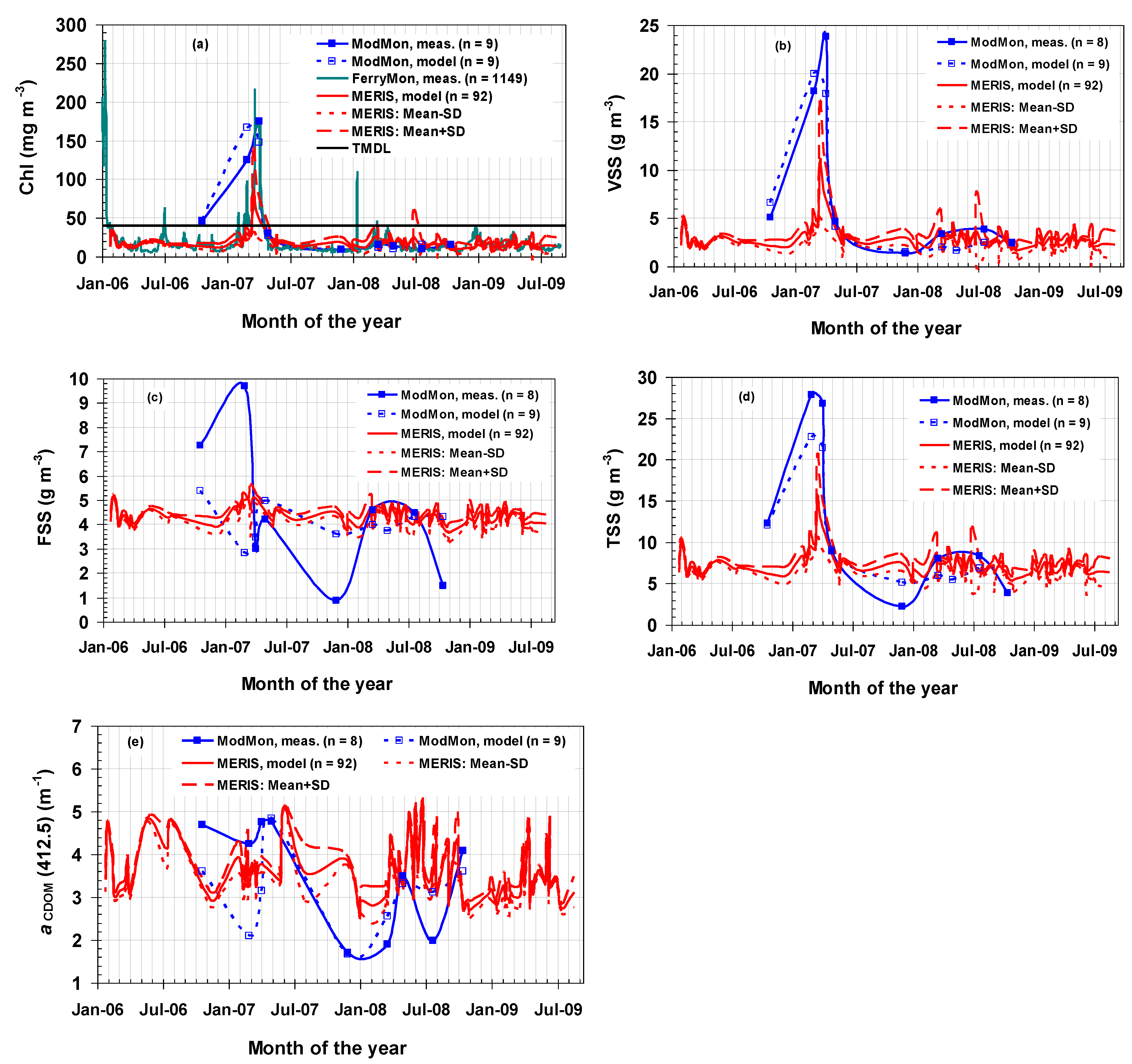
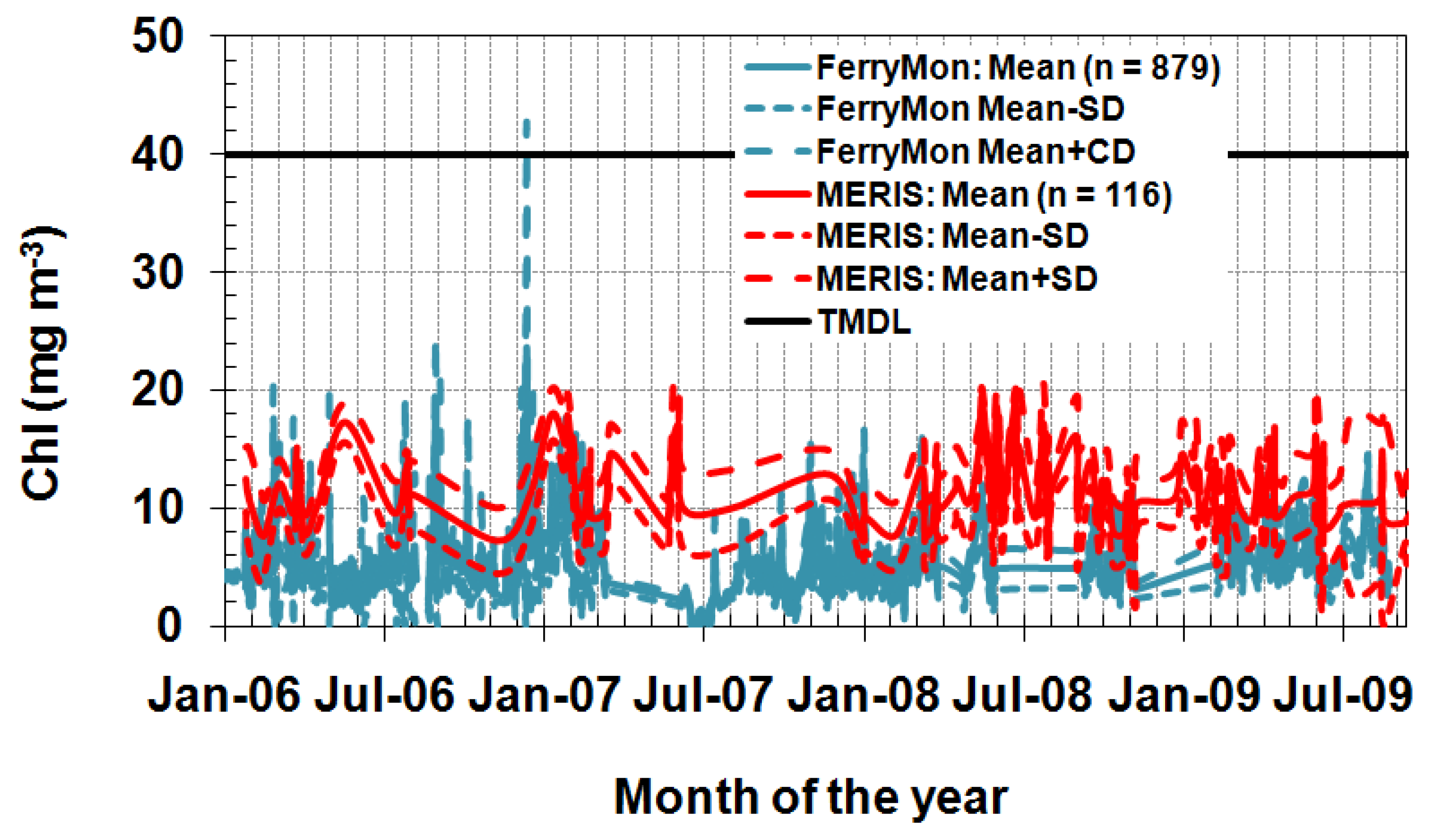
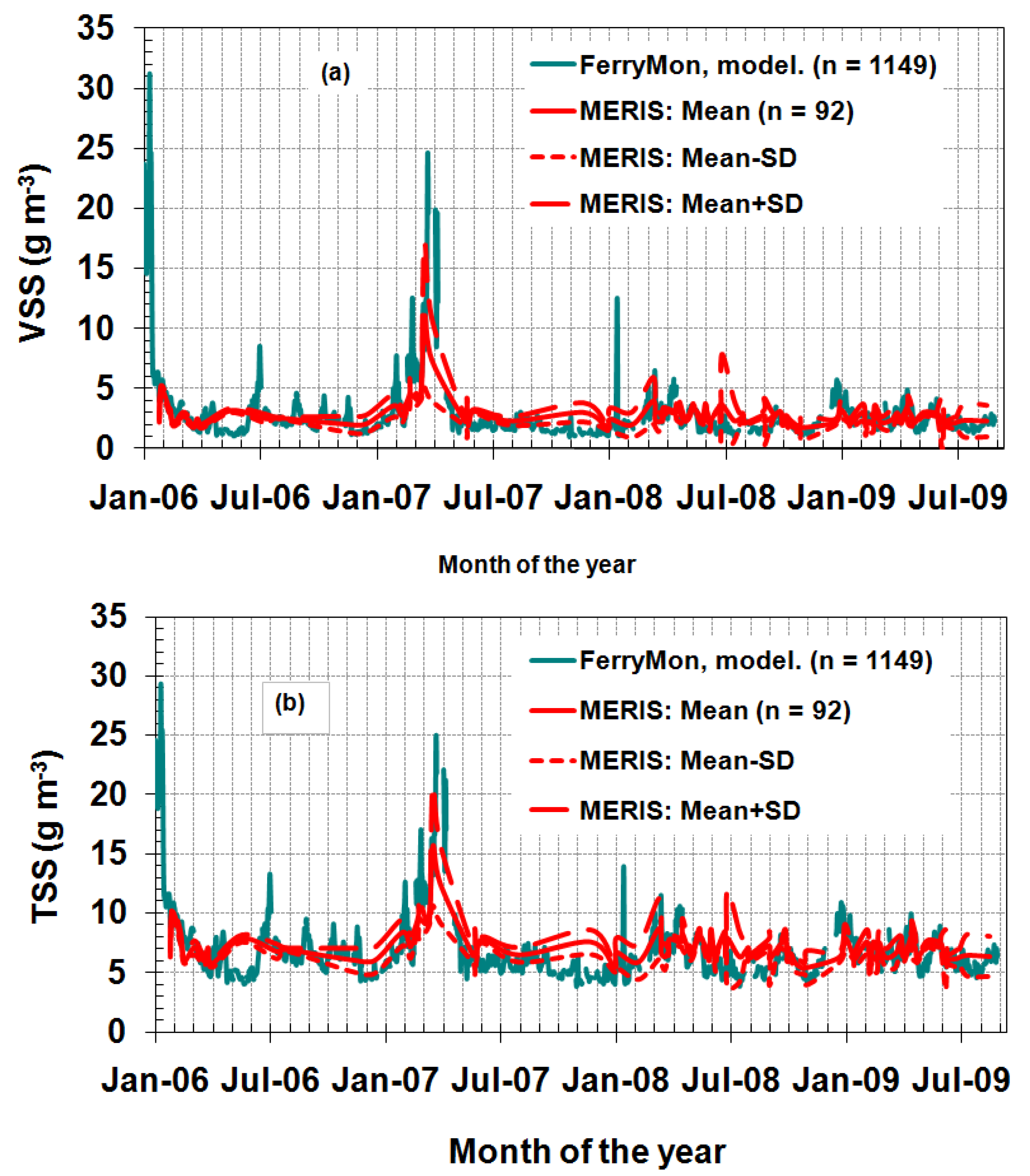
3.3. WQC Dynamics


4. Conclusions
Acknowledgments
References
- Boss, E.; Perry, M.J.; Swift, D.; Taylor, L.; Brickley, P.; Zaneveld, J.R.V. Three years of ocean data from a bio-optical profiling float. Eos Trans. AGU 2008, 89, 209–210. [Google Scholar] [CrossRef]
- Campbell, J.W.; Esaias, W.E. Basis for spectral curvature algorithms in remote sensing of chlorophyll. Appl. Opt. 1983, 22, 1084–1093. [Google Scholar] [CrossRef] [PubMed]
- O’Reilly, J.E.; Maritorena, S.; Mitchell, B.G.; Siegel, D.A.; Carder, K.L.; Garver, S.A.; Kahru, M.; McClain, C. Ocean color chlorophyll algorithms for SeaWiFS. J. Geophys. Res. 1998, 103, 24937–24953. [Google Scholar] [CrossRef]
- Dall’olmo, G.; Gitelson, A.A. Effect of bio-optical parameter variability on the remote estimation of chlorophyll-a concentration in turbid productive waters: Experimental results. Appl. Opt. 2005, 44, 412–422. [Google Scholar] [CrossRef] [PubMed]
- IOCCG. Remote Sensing of Inherent Optical Properties: Fundamentals, Tests of Algorithms, and Applications; Reports of the International Ocean-Colour Coordinating Group, No. 5; Lee, Z., Ed.; IOCCG: Dartmouth, NS, Canada, 2006. [Google Scholar]
- Khorram, S.; Cheshire, H.M. Remote sensing of water quality in the Neuse River Estuary, North Carolina. Photogramm. Eng. Remote Sensing 1985, 51, 329–341. [Google Scholar]
- Woodruff, D.L.; Stumpf, R.P.; Scope, J.A.; Paerl, H.W. Remote estimation of water clarity in optically complex estuarine waters. Remote Sens. Environ. 1999, 68, 41–52. [Google Scholar] [CrossRef]
- Stumpf, R.P.; Pennock, J.R. Remote estimation of the diffuse attenuation coefficient in a moderately turbid estuary. Remote Sens. Environ. 1991, 38, 183–191. [Google Scholar] [CrossRef]
- Gordon, H.R. Simple calculation of the diffuse reflectance of ocean. Appl. Opt. 1973, 12, 2803–2804. [Google Scholar] [CrossRef] [PubMed]
- Haltrin, V.I.; Gallegos, S.C. About nonlinear dependence of remote sensing and diffuse reflection coefficients of Gordon’s parameter. In Proceedings of Conference “Current Problems in Optics of Natural Waters”, St. Petersburg, Russia, 8–12 September 2003; pp. 363–369. Available online: http://vih.freeshell.org/pp/03_ONW_St.Petersburg/Nonlin_RSR.pdf (accessed on 28 March 2011).
- Sokoletsky, L. A comparative analysis of simple radiative transfer approaches for aquatic environments. In Proceedings of the 2004 ENVISAT & ERS Symposium, Salzburg, Austria, 6–10 September 2004. [CD-ROM].
- Twardowski, M.S.; Boss, E.; Macdonald, J.B.; Pegau, W.S.; Barnard, A.H.; Zaneveld, J.R.V. A model for estimating bulk refractive index from the optical backscattering ratio and the implications for understanding particle composition in case I and case II waters. J. Geophys. Res. 2001, 106, 14129–14142. [Google Scholar] [CrossRef]
- Sokoletsky, L. In situ and Remote Sensing Bio-optical Methods for the Estimation of Phytoplankton Concentration in the Gulf of Aqaba (Eilat). Ph.D. Thesis, Bar-Ilan University, Ramat-Gan, Israel, 2003. [Google Scholar]
- Woźniak, S.B.; Stramski, D. Modeling the optical properties of mineral particles suspended in seawater and their influence on ocean reflectance and chlorophyll estimation from remote sensing algorithms. Appl. Opt. 2004, 43, 3489–3503. [Google Scholar] [CrossRef] [PubMed]
- Karaska, M.A.; Huguenin, R.L.; Beacham, J.L.; Wang, M.; Jensen, J.R.; Kaufmann, R.S. AVIRIS measurements of chlorophyll, suspended minerals, dissolved organic carbons, and turbidity in the Neuse River, North Carolina. Photogramm. Eng. Remote Sensing 2004, 70, 125–133. [Google Scholar] [CrossRef]
- Huguenin, R.L.; Wang, M.; Biehl, R.; Stoodley, S.; Rogers, J.N. Automated subpixel photobathymetry and water quality mapping. Photogramm. Eng. Remote Sensing 2004, 70, 111–123. [Google Scholar] [CrossRef]
- Morel, A.; Prieur, L. Analysis of variations in ocean color. Limnol. Oceanogr. 1977, 22, 709–722. [Google Scholar] [CrossRef]
- Dekker, A.G.; Peters, S.W.M. The use of the Thematic Mapper for the analysis of eutrophic lakes: A case study in the Netherlands. Int. J. Remote Sens. 1993, 14, 799–821. [Google Scholar] [CrossRef]
- Kalio, K.; Kutser, T.; Hannonen, T.; Koponen, S.; Pulliainen, J.; Vepsäläinen, J.; Puhälahti, T. Retrieval of water quality from airborne imaging spectrometry of various lake types in different seasons. Sci. Total Environ. 2001, 268, 59–77. [Google Scholar] [CrossRef]
- Doxaran, D.; Froidefond, J.M.; Castaing, P. A reflectance band ratio used to estimate suspended matter concentrations in sediment-dominated coastal waters. Int. J. Remote Sens. 2002, 23, 5079–5085. [Google Scholar] [CrossRef]
- Brezonik, P.; Menken, K.D.; Bauer, M. Landsat-based remote sensing of lake water quality characteristics, including chlorophyll and colored dissolved organic matter (CDOM). Lake Reserv. Manag. 2005, 4, 373–382. [Google Scholar] [CrossRef]
- Morel, A.; Gentili, B. A simple band ratio technique to quantify the colored and detrital organic material from ocean color remotely sensed data. Remote Sens. Environ. 2009, 113, 998–1011. [Google Scholar] [CrossRef]
- Sokoletsky, L.; Gallegos, S. Towards development of an improved technique for remote retrieval of water quality components: An approach based on the Gordon’s parameter spectral ratio. In Proceedings of the Ocean Optics XX Conference, Anchorage, AK, USA, 27 September–1 October 2010. #100881.
- Ruddick, K.G.; Gons, H.J.; Rijkeboer, M.; Tilstone, G. Optical remote sensing of chlorophyll a in case 2 waters by use of an adaptive two-band algorithm with optimal error properties. Appl. Opt. 2001, 40, 3575–3585. [Google Scholar] [CrossRef] [PubMed]
- Gons, H.J.; Rijkeboer, M.; Ruddick, K.G. A chlorophyll-retrieval algorithm for satellite imagery (Medium Resolution Imaging Spectrometer) of inland and coastal waters. J. Plankton Res. 2002, 24, 947–951. [Google Scholar] [CrossRef]
- Lee, Z.P.; Carder, K.L.; Arnone, R.A. Deriving inherent optical properties from water color: A multiband quasi-analytical algorithm for optically deep waters. Appl. Opt. 2002, 41, 5755–5772. [Google Scholar] [CrossRef] [PubMed]
- Peters, S.W.M.; Pasterkamp, R.; van de Woerd, H.J. A sensitivity analysis of analytical inversion methods to derive chlorophyll from MERIS spectra in case-II waters. In Proceedings of the Ocean Optics XVI Conference, Santa Fe, NM, USA, November 2002; pp. 363–369. Available online: http://www.brockmann-consult.de/revamp/pdfs/147.pdf (accessed on 28 March 2011).
- Cauwer, V.D.; Ruddick, K.; Park, Y.J.; Kyramarios, M. Optical remote sensing in support of eutrophication monitoring in the Southern North Sea. EARSeL eProceedings 2004, 3, 208–221. [Google Scholar]
- Craig, S.E.; Lohrenz, S.E.; Lee, Z.P.; Mahoney, K.L.; Kirkpatrick, G.J.; Schofield, O.M.; Steward, R.G. Use of hyperspectral remote sensing reflectance for detection and assessment of the harmful alga, Karenia brevis. Appl. Opt. 2006, 45, 5414–5425. [Google Scholar] [CrossRef] [PubMed]
- Sokoletsky, L.G.; Lunetta, R.S.; Wetz, M.S.; Paerl, H.W. Assessment of the water quality components in turbid estuarine waters based on radiative transfer approximations. 2011; submitted. [Google Scholar]
- Defoin-Platel, M.; Chami, M. How ambiguous is the inverse problem of ocean color in coastal waters? J. Geophys. Res. 2007, 112, C03004. [Google Scholar] [CrossRef]
- Lunetta, R.S.; Knight, J.F.; Paerl, H.W.; Streicher, J.J.; Peierls, B.L.; Gallo, T.; Lyon, J.G.; Mace, T.H.; Buzzelli, C.P. Measurement of water colour using AVIRIS imagery to assess the potential for an operational monitoring capability in the Pamlico Sound Estuary, USA. Int. J. Remote Sens. 2009, 30, 3291–3314. [Google Scholar] [CrossRef] [PubMed]
- Berk, A.; Bernstein, L.S.; Robertson, D.C. MODTRAN: A Moderate Resolution Model for LOWTRAN 7; Technical Report GL-TR-0122; AFGL, Hanscom AFB: Bedford, MA, USA, 1989. [Google Scholar]
- Stamnes, K.; Conklin, P. A new multi-layer discrete ordinate approach to radiative transfer in vertically inhomogeneous atmospheres. J. Quant. Spectrosc. Radiat. Transfer 1984, 31, 273–282. [Google Scholar] [CrossRef]
- Paerl, H.W.; Bales, J.D.; Ausley, L.W.; Buzzelli, C.P.; Crowder, L.B.; Eby, L.A.; Fear, J.M.; Go, M.; Peierls, B.L.; Richardsoni, T.L.; Ramus, J.S. Ecosystem impacts of three sequential hurricanes (Dennis, Floyd, and Irene) on the United States’ largest lagoonal estuary, Pamlico Sound, NC. Proc. Nat. Acad. Sci. USA 2001, 98, 5655–5660. [Google Scholar] [CrossRef] [PubMed]
- Paerl, H.W.; Valdes, L.M.; Joyner, A.R.; Peierls, B.L.; Piehler, M.F.; Riggs, S.R.; Christian, R.R.; Eby, L.A.; Crowder, L.B.; Ramus, J.S.; Clesceri, E.J.; Buzzelli, C.P.; Luettich, R.A. Ecological response to hurricane events in the Pamlico Sound system, North Carolina, and implications for assessment and management in a regime of increased frequency. Estuar. Coast. 2006, 29, 1033–1045. [Google Scholar] [CrossRef]
- Burkholder, J.; Eggleston, D.; Glasgow, H.; Brownie, C.; Reed, R.; Janowitz, G.; Posey, M.; Melia, G.; Kinder, C.; Corbett, R.; Toms, D.; Alphin, T.; Deamer, N.; Springer, J. Comparative impacts of two major hurricane seasons on the Neuse River and western Pamlico Sound ecosystems. Proc. Nat. Acad. Sci. USA 2004, 101, 9291–9296. [Google Scholar] [CrossRef] [PubMed]
- Copeland, B.J.; Gray, J. Status and Trends of the Albemarle-Pamlico Estuary Study; Technical Report 90-01; Department of Environment, Health, and Natural Resources, NC State University: Raleigh, NC, USA, 1991. [Google Scholar]
- Paerl, H.W.; Pinckney, J.L.; Fear, J.M.; Peierls, B.L. Ecosystem responses to internal and watershed organic matter loading: consequences for hypoxia in the eutrophying Neuse River Estuary, North Carolina, USA. Mar. Ecol. Prog. Ser. 1998, 166, 17–25. [Google Scholar] [CrossRef]
- Paerl, H.W.; Valdes, L.M.; Piehler, M.F.; Stow, C.A. Assessing the effects of nutrient management in an estuary experiencing climatic change: The Neuse River Estuary, NC, USA. Environ. Manage. 2006, 37, 422–436. [Google Scholar] [CrossRef] [PubMed]
- Buzzelli, C.P.; Ramus, J.R.; Paerl, H.W. Ferry-based monitoring of surface water quality in North Carolina estuaries. Estuaries 2003, 26, 975–984. [Google Scholar] [CrossRef]
- Mobley, C.D. Estimation of the remote-sensing reflectance from above-surface measurements. Appl. Opt. 1999, 38, 7442–7455. [Google Scholar] [CrossRef] [PubMed]
- Sokoletsky, L. Comparative analysis of selected radiative transfer approaches for aquatic environments. Appl. Opt. 2005, 44, 136–148. [Google Scholar] [CrossRef] [PubMed]
- Paerl, H.W.; Rossignol, K.L.; Hall, N.S.; Guajardo, R.; Joyner, A.R.; Peierls, B.L.; Ramus, J.S. FerryMon: Ferry-based monitoring and assessment of human and climatically-driven environmental change in the Pamlico Sound System, North Carolina, USA. Environ. Sci. Technol. 2009, 43, 7609–7613. [Google Scholar] [CrossRef] [PubMed]
- Curran, P.J.; Steele, C.M. MERIS: The re-branding of an ocean sensor. Int. J. Remote Sens. 2005, 26, 1781–1798. [Google Scholar] [CrossRef]
- Gordon, H.R.; Castaño, D.J. Coastal Zone Color Scanner atmospheric correction algorithm: Multiply scattering effects. Appl. Opt. 1987, 26, 2111–2122. [Google Scholar] [CrossRef] [PubMed]
- Haltrin, V.I. Empirical relationship between aerosol scattering phase function and optical thickness of atmosphere above the ocean. Proc. SPIE 1998, 3433, 334–342. [Google Scholar]
- Gong, S.; Huang, J.; Li, Y.; Wang, H. Comparison of atmospheric correction algorithms for TM image in inland waters. Int. J. Remote Sens. 2008, 29, 2199–2210. [Google Scholar] [CrossRef]
- Katsev, I.L.; Prikhach, A.S.; Zege, E.P.; Ivanov, A.P.; Kokhanovsky, A.A. Iterative procedure for retrieval of spectral aerosol optical thickness and surface reflectance from satellite data using fast radiative code and its application to MERIS measurements. In Satellite Aerosol Remote Sensing over Land; Kokhanovsky, A.A., de Leeuw, G., Eds.; Springer-Praxis: Berlin, Germany, 2009; pp. 101–134. [Google Scholar]
- Albert, A.; Gege, P. Inversion of irradiance and remote sensing reflectance in shallow water between 400 and 800 nm for calculations of water and bottom properties. Appl. Opt. 2006, 45, 2331–2343. [Google Scholar] [CrossRef] [PubMed]
- Mishchenko, M.I.; Dlugach, J.M.; Yanovitskij, E.G.; Zakharova, N.T. Bidirectional reflectance of flat, optically thick particulate layers: An efficient radiative transfer solution and applications to snow and soil surfaces. J. Quant. Spectrosc. Radiat. Transfer 1999, 63, 409–432. [Google Scholar] [CrossRef]
- Kokhanovsky, A.A.; Sokoletsky, L.G. Reflection of light from semi-infinite absorbing turbid media. Part 1: Spherical albedo. Color Res. Appl. 2006, 31, 491–497. [Google Scholar] [CrossRef]
- Kokhanovsky, A.A.; Sokoletsky, L.G. Reflection of light from semi-infinite absorbing turbid media. Part 2: Plane albedo and reflection function. Color Res. Appl. 2006, 31, 498–509. [Google Scholar] [CrossRef]
- Sokoletsky, L.G.; Nikolaeva, O.V.; Budak, V.P.; Bass, L.P.; Lunetta, R.S.; Kuznetsov, V.S.; Kokhanovsky, A.A. Comparison of different numerical and analytical solutions of the radiative-transfer equation for plane albedo with emphasis on the natural waters consideration. J. Quant. Spectrosc. Radiat. Transfer 2009, 110, 1132–1146. [Google Scholar] [CrossRef]
- Petzold, T.J. Volume Scattering Functions for Selected Ocean Waters; Technical Report SIO 72-78; Scripps Institution of Oceanography: San Diego, CA, USA, 1972. [Google Scholar]
- Haltrin, V.I. An analytical Fournier-Forand scattering phase function as an alternative to the Henyey-Greenstein phase function in hydrologic optics. Proc. IEEE 1998, 11, 910–913. [Google Scholar]
- Mobley, C.D.; Sundman, L.K.; Boss, E. Phase function effects on oceanic light fields. Appl. Opt. 2002, 41, 1035–1050. [Google Scholar] [CrossRef] [PubMed]
- Hapke, B. Theory of Reflectance and Emittance Spectroscopy; Cambridge University Press: New York, NY, USA, 1993. [Google Scholar]
- Knaeps, E.; Sterckx, S.; Raymaekers, D. A seasonally robust empirical algorithm to retrieve suspended sediment concentrations in the Scheldt River. Remote Sens. 2010, 2, 2040–2059. [Google Scholar] [CrossRef]
- Hooker, S.B.; Esaias, W.E.; Feldman, G.C.; Gregg, W.W.; McClain, C.R. An overview of SeaWiFS and ocean color. In SeaWiFS Technical Report Series, NASA Technical Memorandum 104566; Hooker, S.B., Firestone, E.R., Eds.; NASA Goddard Space Flight Center: Greenbelt, MD, USA, 1992; Volume 1, pp. 1–24. [Google Scholar]
- Mueller, J.L.; Austin, R.W.; Fargion, G.S.; McClain, C.R. Ocean color radiometry and bio-optics. In Ocean Optics Protocols for Satellite Ocean Color Sensor Validation; Mueller, J.L., Fargion, G.S., Eds.; NASA/TM-2003-21621, Revision 4; NASA Goddard Space Flight Center: Greenbelt, MD, USA, 2003; Volume 1. [Google Scholar]
- Borsuk, M.E.; Stow, C.A.; Reckhow, K.H. Integrated approach to Total Maximum Daily Load development for Neuse River Estuary using Bayesian Probability Network Model (Neu-BERN). J. Water Res. Plan. Manage. 2003, 131, 271–282. [Google Scholar] [CrossRef]
- Smith, E.T.; Zhang, H.X. Developing key water quality indicators for sustainable water resources management. In Proceedings of 77th Annual Water Environment Federation Technical Exhibition and Conference, New Orleans, LA, USA, 2–6 October 2004; Available online: http://acwi.gov/swrr/Rpt_Pubs/WEFTEC04_SWRR_Zhang.pdf (accessed on 28 March 2011).
- Rigollier, C.; Bauer, O.; Wald, L. On the clear sky model of the 4th European Solar Radiation Atlas with respect to the Heliosat method. Solar Energy 2000, 68, 33–48. [Google Scholar] [CrossRef]
- Aboura, R.; Lansari, A. Satellite-derived surface radiation budget over the Algerian area. In Proceedings of the International Congress on Photovoltaic and Wind Energy (ICPWE'03), Tlemcen, Algeria, 16–18 December 2003; Available online: http://www.cder.dz/download/Art02.pdf (accessed on 28 March 2011).
- Remund, J.; Wald, L.; Lefèvre, M.; Ranchin, T.; Page, J. Worldwide linke turbidity information. In Proceedings of the ISES Solar World Congress, Göteborg, Sweden, 16–19 June 2003; Available online: http://www.meteotest.ch/fileadmin/user_upload/Sonnenenergie/pdf/Remund_ises2003_linketurbidity.pdf (accessed on 28 March 2011).
- Remund, J.; Kunz, S.; Schilter, C. Handbook of METEONORM, version 6.114. Part II: Theory; METEOTEST: Bern, Switzerland, 2009; Available online: http://www.meteonorm.com/media/pdf/mn6_theory.pdf (accessed on 28 March 2011).
- Spencer, J.W. Fourier series representation of the position of the sun. Search 1971, 2, 272. [Google Scholar]
- Kasten, F.; Young, A.T. Revised optical air mass tables and approximation formula. Appl. Opt. 1989, 28, 4735–4738. [Google Scholar] [CrossRef] [PubMed]
- Exell, R.H.B. A mathematical model for solar radiation in South-East Asia (Thailand). Solar Energy 1981, 26, 161–168. [Google Scholar] [CrossRef]
- Duffie, J.A.; Beckman, W.A. Solar Engineering of Thermal Processes; Wiley: New York, NY, USA, 1991. [Google Scholar]
- Helyar, A.G. Equation of time. 2001. Available online: http://homepages.pavilion.co.uk/aghelyar/sundat.htm (accessed on 28 March 2011).
- Sekera, Z. Reciprocity relations for diffuse reflection and transmission of radiative transfer in the planetary atmosphere. Astrophys. J. 1970, 162, 3–16. [Google Scholar] [CrossRef]
- Yang, H.; Gordon, H.R. Remote sensing of ocean color: assessment of water-leaving radiance bidirectional effects on atmospheric diffuse transmittance. Appl. Opt. 1997, 36, 7887–7897. [Google Scholar] [CrossRef] [PubMed]
- Thuillier, G.; Herse, M.; Simon, P.C.; Labs, D.; Mandel, H.; Gillotay, D.; Foujols, T. The solar spectral irradiance from 200 to 2400 nm as measured by the SOLSPEC spectrometer from the ATLAS 1-2-3 and EURECA missions. Solar Phys. 2003, 214, 1–22. [Google Scholar] [CrossRef]
- Toole, D.A.; Siegel, D.A.; Menzies, D.W.; Neumann, M.J.; Smith, R.C. Remote-sensing reflectance determinations in the coastal ocean environment: Impact of instrumental characteristics and environmental variability. Appl. Opt. 2000, 39, 456–469. [Google Scholar] [CrossRef] [PubMed]
- Sokoletsky, L.G.; Oren, A.; Stambler, N.; Iluz, D. Practical algorithms for remote-sensing retrieval of the water column constituents in the Israeli waters. In Proceedings of Conference “Current Problems in Optics of Natural Waters”, St. Petersburg, Russia, 8–12 September 2009.
- Ruddick, K.G.; Cauwer, V.D.; Park, Y.J. Seaborne measurements of near infrared water-leaving reflectance: The similarity spectrum for turbid waters. Limnol. Oceanogr. 2006, 51, 1167–1179. [Google Scholar] [CrossRef]
Appendix A
Atmospheric Correction Equations
© 2011 by the authors; licensee MDPI, Basel, Switzerland. This article is an open access article distributed under the terms and conditions of the Creative Commons Attribution license (http://creativecommons.org/licenses/by/3.0/).
Share and Cite
Sokoletsky, L.G.; Lunetta, R.S.; Wetz, M.S.; Paerl, H.W. MERIS Retrieval of Water Quality Components in the Turbid Albemarle-Pamlico Sound Estuary, USA. Remote Sens. 2011, 3, 684-707. https://doi.org/10.3390/rs3040684
Sokoletsky LG, Lunetta RS, Wetz MS, Paerl HW. MERIS Retrieval of Water Quality Components in the Turbid Albemarle-Pamlico Sound Estuary, USA. Remote Sensing. 2011; 3(4):684-707. https://doi.org/10.3390/rs3040684
Chicago/Turabian StyleSokoletsky, Leonid G., Ross S. Lunetta, Michael S. Wetz, and Hans W. Paerl. 2011. "MERIS Retrieval of Water Quality Components in the Turbid Albemarle-Pamlico Sound Estuary, USA" Remote Sensing 3, no. 4: 684-707. https://doi.org/10.3390/rs3040684
APA StyleSokoletsky, L. G., Lunetta, R. S., Wetz, M. S., & Paerl, H. W. (2011). MERIS Retrieval of Water Quality Components in the Turbid Albemarle-Pamlico Sound Estuary, USA. Remote Sensing, 3(4), 684-707. https://doi.org/10.3390/rs3040684