Abstract
With the progression of LiDAR (Light Detection and Ranging) towards a mainstream resource management tool, it has become necessary to understand how best to process and analyze the data. While most ground surface identification algorithms remain proprietary and have high purchase costs; a few are openly available, free to use, and are supported by published results. Two of the latter are the multiscale curvature classification and the Boise Center Aerospace Laboratory LiDAR (BCAL) algorithms. This study investigated the accuracy of these two algorithms (and a combination of the two) to create a digital terrain model from a raw LiDAR point cloud in a semi-arid landscape. Accuracy of each algorithm was assessed via comparison with >7,000 high precision survey points stratified across six different cover types. The overall performance of both algorithms differed by only 2%; however, within specific cover types significant differences were observed in accuracy. The results highlight the accuracy of both algorithms across a variety of vegetation types, and ultimately suggest specific scenarios where one approach may outperform the other. Each algorithm produced similar results except in the ceanothus and conifer cover types where BCAL produced lower errors.
1. Introduction
Developing accurate Digital Terrain Models (DTM) has been a long stated goal of both researchers and resource managers interested in quantifying land surface elevations. The potential applications of a reliable DTM include habitat assessment, forest succession, snowmelt simulation, hydrologic modeling, carbon sequestration, glacial monitoring, and floodplain assessments [1,2,3,4,5,6]. Prior to the introduction of Light Detection and Ranging (LiDAR), traditional methods such as photogrammetry and field surveys were conducted to produce DTMs. While these methods can generate DTMs with acceptable levels of accuracy for certain applications, both methods are time and labor intensive. Furthermore, in the presence of steep slopes or high biomass, traditional DTM generation methods are difficult to implement, often leading to reduced levels of accuracy [7,8,9]. Research has demonstrated that LiDAR DTM generation is more efficient and accurate as compared to traditional methods [10]. The creation of accurate DTMs is vital to understand the reliability of other LiDAR-derived metrics, such as canopy cover, tree heights, and leaf area index [11].
In recent years investigations have focused on the influence of environmental conditions (e.g., slope, elevation, cover type) and sensor characteristics (e.g., flight height, point density, and scan angles) on the accuracy of LiDAR-derived DTMs [2,12,13,14,15,16,17,18,19], ultimately demonstrating the reliability of LiDAR-derived DTMs across a range of terrain and cover types with varying acquisition parameters. Other studies investigated the impact that different point interpolators have on the accuracy of LiDAR‑derived DTMs [20,21]. Most suggest that when the LiDAR acquisition has an adequate pulse density, usually equal to, or denser than the desired DTM resolution (cell size), there are only negligible differences in accuracy due to interpolation methods. These past studies provided insight into the reliability of LiDAR to create accurate DTMs in various landscape types and have developed guidelines for working with LiDAR in different ecosystems [22].
Raw LiDAR point clouds contain returns from both ground and non-ground objects. Classification of these points as ground or non-ground returns is the first step in generating a DTM from LiDAR data. Although the influence of different variables like pulse density, terrain slope, and vegetation on the vertical accuracy of LiDAR-derived DTMs has been assessed, little attention has been paid to the accuracies of the different point classification algorithms commonly being applied. Point classification algorithms that are commonly applied by LiDAR vendors are considered proprietary knowledge, are often grey- or black-box approaches, and thus are not readily available for independent validation and comparison. For landowners that will only every acquire LiDAR once or twice, the use of these proprietary methodologies is limited by the high cost of purchasing the software ($5,000–$20,000). However, in recent years open source point classification algorithms have been developed. Since they are open source, such algorithms can be independently tested, evaluated, and compared against the products commonly produced by vendors. Two such algorithms are the Multiscale Curvature Classification LiDAR algorithm (MCC, http://sourceforge.net/project/mccLiDAR) and the Boise Center Aerospace Laboratory LiDAR algorithm (BCAL).
The MCC algorithm was developed at the Moscow Forestry Sciences Laboratory of the USFS Rocky Mountain Research Station [23] and the BCAL algorithm was developed by the Boise Center Aerospace Laboratory of Idaho State University [24]. The two algorithms were developed for different objectives; MCC was intended for classifying LiDAR returns in high biomass forest ecosystems [2,25,26,27,28], while the BCAL algorithm was developed specifically for optimal performance in shrub-steppe ecosystems [19,24,29,30]. The primary difference between the way the methods iteratively interpolate surfaces to the point cloud during processing is that MCC works from the top down while BCAL works from the bottom up. The MCC algorithm operates by discarding returns that exceed a threshold curvature calculated from a surface interpolated using a thin plated spline. Through three successively larger scale domains that define the processing window size, the algorithm iterates until the number of remaining returns changes by <1%, <0.1% and finally <0.01% for the three scale domains, respectively [23]. BCAL is a grid based classification algorithm, first identifying the lowest elevation point in a search area determined by the user, and then creating a surface by interpolating these lowest points [24]. In subsequent iterations, any point that lies on or below the previous iteration’s surface are classified as ground points and are included in subsequent iterations. The iterations continue until there are no unclassified returns below the interpolated surface in which case all unclassified returns above the surface are classified as vegetation returns.
The objective of this study is to cross compare and evaluated the ability of the two algorithms to filter a raw LiDAR point cloud and produce an accurate DTM in a semi-arid watershed with mixed vegetation types. The performance of each algorithm is tested for overall accuracy, in a variety of cover types and at different spatial resolutions.
2. Methods
2.1. Study Area
The study area is the 38 ha Reynolds Mountain East (RME) catchment, which is part of the larger Reynolds Creek Experimental Watershed (Figure 1). Located in southwestern Idaho, USA, the watershed is owned by the Bureau of Land Management and research infrastructure in the watershed is managed by the USDA ARS Northwest Watershed Research Center. The catchment is in a semi-arid mountainous area ranging from 2,023 to 2,139 m in elevation with slopes reaching 35°. The landscape is a patchwork of shrub-steppe, meadow, and bare ground with large stands of coniferous and deciduous forests that occur in topographically sheltered zones. The shrub-steppe in RME is dominated by mountain big sagebrush (Artimesia tridentate Nutt. ssp. vaseyana) and mountain snowberry (Symphoricarpos oreophilus Gray) with patches of prostrate ceanothus (Ceanothus prostratus Benth.). The meadow is a mixture of forbs and graminoids with Lupinus ssp. and Carex ssp. dominating the forbs and Poa ssp. dominating the graminoids. The conifer tree stand is solely comprised of Douglas-fir (Pseudotsuga menziesii), while quaking aspen (Populus tremuloides) dominates the deciduous stand.
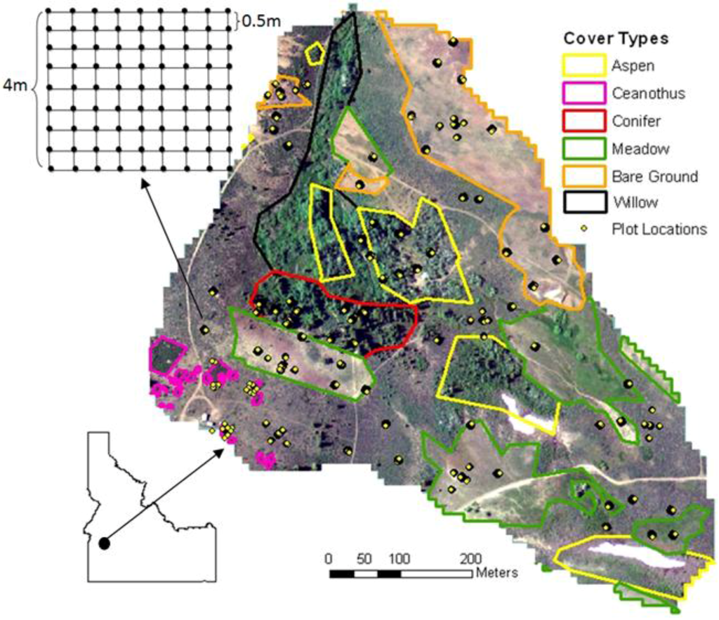
Figure 1.
Cover type map of Reynolds Creek Mountain East, defined by seven classes (Willow, Ceanothus, Shrub, Bare Ground, Conifer, Meadow, and Aspen). The shrub cover type represents all areas not outlined by other cover types and the willow cover type was excluded from surveying due to the impracticality of operating equipment in saturated areas. Each set of yellow points represents the location of a 4 m by 4 m plot with survey points systematically gridded every 0.5 m (81 points/plot; 9 points/m2; see inset).
2.2. LiDAR Data and Acquisition
Airborne LiDAR data were acquired in mid-November 2007 with a Leica ALS50 Phase II Laser, which operated at a wavelength of 1,064 nm and records up to four returns per pulse. The data were acquired with a nominal pulse density of 6 pulses/m2 and an off nadir scan angle of ±15°. The mean return rate and range of return rates across the study area were 5.7 returns/m2 and 0–70 returns/m2, respectively. According to vendor provided measurements, the absolute vertical accuracy in terms of root mean square error (RMSE) was 3.3 cm based on 1,002 real time kinematic (RTK) global positioning system (GPS) points surveyed on asphalt road surfaces throughout the watershed. The flight lines were calibrated and the raw LiDAR data were tiled using the TerraScan and TerraMatch software respectively (Terrasolid Ltd., Jyväskylä, Finland), the delivered raw bins were projected in NAD83 UTM Zone 11 North. Along with the xyz coordinates, GPS time, intensity, and scan angle were also recorded for each return. A study using the same LiDAR dataset, from another area of the watershed, found a vertical accuracy of approximately 10 cm and horizontal accuracy within 30 cm [29].
2.3. Point Classification with MCC and BCAL
The raw LiDAR point cloud was classified into ground and non-ground returns with both of the previously described algorithms (MCC and BCAL). Ranges for initial parameters were selected for both methods by consulting with the algorithm developers, for MCC the scale and curvature ranged from 0.8 to 1.5 and 0.01–0.10, respectively, and for BCAL the window and threshold ranged from 5 to 7 m and 0.00–0.10 m, respectively. These initial parameters were used to produce DTMs for an optimization process in order to determine which parameter settings produce the lowest root mean square error (RMSE) for the study area. We acknowledge that a similar optimization process will be necessary for other study areas, especially with different vegetation types such as forests. The MCC parameters found to operate the best were a scale value of 1.0 and curvature value of 0.05. Both the original BCAL algorithm and a modified version were applied to the raw LiDAR data set. In the modified BCAL algorithm, a threshold level is applied, which instead of classifying LiDAR returns using the absolute interpolated surface, the interpolated surface plus a threshold value of 0.05–0.10 m was used at each iteration for classifying LiDAR data into ground and non-ground returns. The threshold was applied to allow for an increase in the proportion of returns being classified as ground returns. Through the parameterization process the modified BCAL algorithm was found to outperform the original at all tested resolution levels. The modified algorithm produced the lowest RMSE when the window size was set to 7 m and the threshold value was 0.10 m. Then combinations of the MCC and the modified BCAL algorithms were also applied for filtering the raw point cloud, it was found that using the BCAL window size of 7 m and threshold of 0.10 m with the MCC scale value of 1.0 and a curvature value of 0.05, produced the lowest RMSE of the combined filtering results. This new point classification method will be referred to as Combo through the rest of the paper. The algorithm parameters that are utilized in the analysis are summarized in Table 1.

Table 1.
Finalized algorithm parameters for analysis.
| Algorithm | BCAL Parameters | MCC Parameters | ||
|---|---|---|---|---|
| Window | Threshold | Scale | Curvature | |
| BCAL | 7 m | 0.10 m | – | – |
| MCC | – | – | 1.0 | 0.05 |
| Combo | 7 m | 0.10 m | 1.0 | 0.05 |
2.4. Ground Reference Data
In summer 2010, 71 plot locations were proportionally allocated by area, within six vegetation cover type strata (shrub, ceanothus, meadow, bare ground, deciduous, and conifer; Figure 1). The sampling protocol ensured that the selected plots covered the range of terrain and vegetation variability within the study area (Table 2). Each plot consisted of a 4 × 4 m square within which survey points were systematically distributed on a 0.5 m grid spacing (81 survey points per plot). Each survey point was located and measured (x, y, z position) using a Topcon GTS-236w laser total station that had been georeferenced using a Topcon Hyper-Pro real-time kinematic (RTK) global positioning system (Topcon Corp., Livermore, CA, USA) and the system of USGS monuments (Figure 1). The Topcon Hyper-Pro RTK has a static reading standard of ±15 mm vertical and ±10 mm horizontal. At each of the 81 survey points within the grid a presence/absence of vegetative cover was recorded for calculating the average vegetation cover of the plot (Table 2). In addition to the 81 survey points, additional survey measurements were taken at the center of each shrub (center of crown area) and on the northern side of each tree bole in those plots with trees. This provided a total of 7,285 points for assessing the accuracies of the DTMs.
Table 2.
Distribution of plots within different cover and terrain conditions.
| Cover Type | N | Mean Slope | Max. Slope | Min. Slope | Mean Cover | Max. Cover | Min. Cover |
|---|---|---|---|---|---|---|---|
| Meadow | 19 | 8.2 | 16.9 | 4.2 | 82% | 100% | 14% |
| Shrub | 20 | 7.9 | 15.3 | 3.5 | 96% | 100% | 84% |
| Bare Ground | 10 | 6.8 | 11.8 | 2.6 | 24% | 100% | 0% |
| Ceanothus | 3 | 8.9 | 12.5 | 6.1 | 96% | 100% | 91% |
| Aspen | 9 | 6.5 | 9.5 | 3.9 | 66% | 84% | 39% |
| Conifer | 10 | 12.4 | 17.9 | 7.4 | 79% | 100% | 48% |
*all slopes are given in degrees.
Once the LiDAR point cloud had been classified into ground and non-ground returns with the different combinations of the algorithms and parameters, DTMs were generated from the ground returns via a natural neighbors interpolator. DTMs were generated at 1.0 and 0.5 m cell size resolutions for each of the three algorithms (MCC, BCAL, Combo). It is believed that with the density of returns in this LiDAR data set that error introduced through interpolation is negligible no matter what interpolator is being used [20,21]. The survey point locations were used to extract the corresponding DTM elevations for comparison. The corresponding surveyed elevations were then subtracted from the DTM elevations and these values were analyzed using the Kruskal-Wallis one-way ANOVA. Utilizing the ANOVA, all 7,285 survey points were used to assess the overall performance of the DTM in terms of RMSE across the catchment. Furthermore, the DTMs were analyzed to evaluate which method performed the best within each of the cover types. All results are reported at a significance level of p < 0.05.
3. Analysis and Results
3.1. 1.0 m Resolution
When assessing the overall performance of the algorithms, BCAL, MCC and the Combo returned RMSEs of 27.33, 27.98, and 30.41 cm, respectively. The ANOVA indicated that there was no significant difference between BCAL and MCC, but that each outperformed the Combo algorithm. We further compared the performance of the algorithms within each of the cover types (Figure 2) and observed that BCAL was either comparable to (or significantly better than) the other two methods in each of the cover types. At 1 m resolution, BCAL provided the most consistent performance between the cover types; however, the difference in RMSE between BCAL and MCC overall was only 0.65 cm, an increase of 2.4%. The ceanothus class was the only one where a substantial deviation (~40 cm) occurs between the BCAL and MCC DTMs, it appeared that MCC misclassified several vegetation returns. In other areas, however, it was evident that BCAL removed ground returns from rock outcroppings that MCC had done a better job of retaining, this misclassification caused BCAL’s DTM surface to be nearly 2 m below actual.
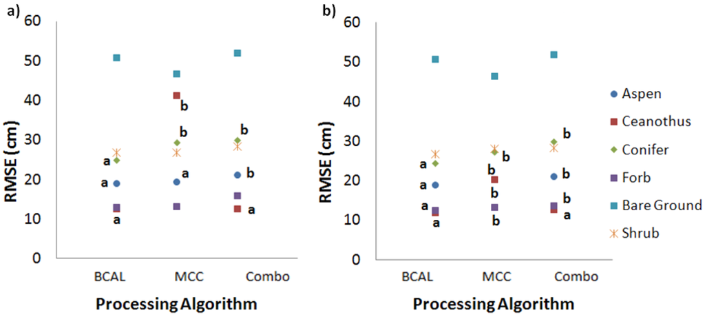
Figure 2.
The three Digital Terrain Models (DTMs) at 1.0 m (a) and 0.5 m (b) were tested to identify the best overall performance in each of the cover types. At 1.0 m resolution there were no significant differences reported in the shrub, forb and bare ground cover types, nor were there significant differences within the shrub and bare ground cover types at 0.5 m resolution. Significance was tested at the p = 0.05 level.
3.2. 0.5 m Resolution
At 0.5 m resolution, BCAL, MCC and the Combo returned overall RMSE levels of 27.18, 27.65, and 28.90 cm, respectively. Again the ANOVA indicated no significant difference between BCAL and MCC, and that both slightly outperformed the Combo algorithm. When testing the algorithms within the different cover types, BCAL outperformed both MCC and the Combo in all of the cover types except the bare ground and shrub classes (Figure 2). At 0.5 m resolution, BCAL provided only marginally better accuracy, with a 0.47 cm or 1.75% increase in RMSE between BCAL and MCC.
These two algorithms were further investigated by comparing the MCC and BCAL DTMs, at the 0.5 m cell size, with a surface created from the grid of plot points, to show the differences between specific scenarios (Figure 3). Image (a) of Figure 3 indicates the challenge of filtering rock outcrops. In this case, when subtracting the survey produced surface from the algorithm surfaces, BCAL had a mean and standard deviation of −92 and 74 cm, while MCC had a mean and standard deviation of −61 and 46 cm. BCAL removed returns that fell on rock outcrops, causing the DTM surface to be more than 2 m below the ‘Truth Surface’. Image (b) demonstrates how the methods perform in the dense vegetation of the ceanothus. In this case, BCAL had a mean and standard deviation of −17 and 5 cm, while MCC had a mean and standard deviation of 20 and 13 cm. Within the ceanothus class it appears that MCC failed to filter much of the vegetation returns from the ground returns. Overall the performance of BCAL and MCC produce comparable DTMs, although they differ in ways that reflect their contrasting processing approaches. MCC caused commission errors with its misclassification of some vegetation returns as ground, while BCAL produced omission errors by omitting some actual terrain features.
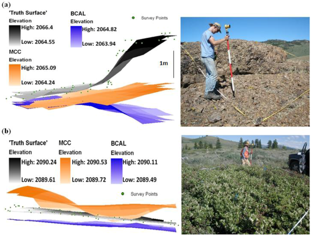
Figure 3.
Surface comparison of the Boise Center Aerospace Laboratory LiDAR algorithm (BCAL), Multiscale Curvature Classification LiDAR algorithm (MCC) and ‘Truth Surface’, created from the 81 survey locations within the plot, for the bare ground (a) and ceanothus (b) cover types. All surfaces are at 0.5 m resolution and elevations are given in meters.
4. Conclusions
This study assessed the potential of the BCAL and MCC algorithms to perform in a mixed cover type landscape with a variety of terrain features. Ideally, multiple algorithms could be applied to different cover types if a highly accurate DTM is required. Table 3 summarizes the performance of each algorithm within the different cover types, these results should be used in deciding which processing method will work the best within a LiDAR acquisition. It can be seen that both BCAL and MCC performed well overall, but BCAL performed better within the ceanothus and conifer cover types. It should be noted that both algorithms tended to produce surfaces with negative elevation biases when compared with the survey points, meaning that predicted elevations were less than those observed. This trend was consistent for all cover types except the ceanothus as predicted by MCC, here there is a large positive bias due to MCC’s failure to classify points within this dense mat of vegetation. The points returned by vegetation like ceanothus (Figure 3(b)) create a plainer feature that MCC is unable to filter, while the block minimum approach that BCAL utilizes is able to remove most of these features.
Separate assessments at both the 1.0 m and 0.5 m resolution level revealed no significant difference between the BCAL and MCC accuracy levels, while both algorithms outperformed the Combo algorithm. The DTM results were also compared between the 1.0 m and 0.5 m resolutions; again this showed no significant difference in accuracy for any of the algorithms/methods. However, it was observed in the DTMs that Combo did experience the greatest improvement in accuracy in each of the cover types and overall, when going from 1.0 m to 0.5 m resolution. The improvement is attributed to the higher percentage of points that MCC retains during classification.
Table 3.
Comparison of algorithm performance overall and within different cover types.
| Cover Type | BCAL | MCC | ||||
|---|---|---|---|---|---|---|
| Mean Error | Std. Dev. Error | Rank | Mean Error | Std. Dev. Error | Rank | |
| Aspen | −0.151 | 0.116 | 1 | −0.149 | 0.122 | 1 |
| Ceonothus | −0.012 | 0.125 | 1 | 0.342 | 0.229 | 2 |
| Conifer | −0.160 | 0.190 | 1 | −0.085 | 0.280 | 2 |
| Forb | −0.058 | 0.116 | 1 | −0.061 | 0.116 | 1 |
| Rock | −0.270 | 0.429 | 1 | −0.248 | 0.395 | 1 |
| Shrub | −0.052 | 0.263 | 1 | −0.046 | 0.265 | 1 |
| Overall | −0.106 | 0.252 | 1 | −0.079 | 0.268 | 1 |
*all accuracies are reported in meters
Both algorithms have potential to be applied to most cover types but one may outperform the other in specific scenarios. The results indicate that BCAL is able to create a more reliable surface in very dense, continuous vegetation like that which occurs in the ceanothus and willow cover types. This is most likely due to the block minimum approach that BCAL uses, allowing it to create a surface from fewer points than MCC. In areas where steep or sudden changes in slope, such as with the rock outcroppings, MCC is expected to outperform BCAL because it retains more ground returns during the filtering process. Although the ANOVA indicates that BCAL and MCC will provide similar overall accuracies when optimally parameterized, a prior knowledge of the terrain and vegetation within a LiDAR acquisition area, and the particular project objective(s), should be considered when deciding which algorithm to employ. Further analysis will be necessary to fully understand how versatile these algorithms are or if they can truly be applied to all landscapes.
Acknowledgments
We thank N. Brewer, J. Hyde, T. Erickson, and Eder Moreira for their contribution to the field survey, Watershed Sciences, Inc. for the LiDAR data acquisition, and the ARS-Northwest Watershed Research Centre technicians for field assistance. This study is supported by the NSF Idaho EPSCoR Program and by the NSF under award numbers EPS-0814387 and CBET-0854553.
References
- Martinuzzi, S.; Vierling, L.A.; Gould, W.A.; Falkowski, M.J.; Evans, J.S.; Hudak, A.T.; Vierling, K.T. Mapping snags and understory shrubs for a lidar-based assessment of wildlife habitat suitability. Remote Sens. Environ. 2009, 113, 2533–2546. [Google Scholar] [CrossRef]
- Falkowski, M.J.; Evans, J.S.; Martinuzzi, S.; Gessler, P.E.; Hudak, A.T. Characterizing forest succession with lidar data: An evaluation for the Inland Northwest, USA. Remote Sens. Environ. 2009, 113, 946–956. [Google Scholar] [CrossRef]
- Essery, R.; Bunting, P.; Hardy, J.; Link, T.; Marks, D.; Melloh, R.; Pomeroy, J.; Rowlands, A.; Rutter, N. Radiative transfer modeling of a coniferous canopy characterized by airborne remote sensing. J. Hydrometeorol. 2008, 9, 228–241. [Google Scholar] [CrossRef]
- Asner, G.P. Tropical forest carbon assessment: Integrating satellite and airborne mapping approaches. Environ. Res. Lett. 2009, 4, 1–11. [Google Scholar] [CrossRef]
- Abermann, J.; Fischer, A.; Lambrecht, A.; Geist, T. On the potential of very high-resolution repeat DEMs in glacial and periglacial environments. The Cryosphere 2010, 4, 53–65. [Google Scholar] [CrossRef]
- Marks, K.; Bates, P. Integration of high-resolution topographic data with floodplain flow models. Hydrol. Process. 2000, 14, 2109–2112. [Google Scholar] [CrossRef]
- Hodgson, M.E.; Jensen, J.; Raber, G.; Tullis, J.; Davis, B.A.; Thompson, G.; Schuckman, K. An evaluation of lidar-derived elevation and terrain slope in leaf-off conditions. Photogramm. Eng. Remote Sensing 2005, 71, 817–823. [Google Scholar] [CrossRef]
- Hollaus, M.; Wagner, W.; Eberhofer, C.; Karel, W. Accuracy of large-scale canopy heights derived from lidar data under operational constraints in a complex alpine environment. ISPRS J. Photogram. Remote Sens. 2006, 60, 323–338. [Google Scholar] [CrossRef]
- Baltsavias, E.P. Airborne laser scanning: Existing systems and firms and other resources. ISPRS J. Photogram. Remote Sens. 1999, 54, 165–198. [Google Scholar] [CrossRef]
- Hodgson, M.E.; Jenson, J.R.; Schmidt, L.; Schill, S.; Davis, B. An evaluation of lidar- and IFSAR-derived digital elevation models in leaf-on conditions with USGS Level 1 and Level 2 DEMs. Remote Sens. Environ. 2003, 84, 295–308. [Google Scholar] [CrossRef]
- Smith, S.L.; Holland, D.A.; Longley, P.A. The importance of understanding error in lidar digital elevation models. In Proceedings of XXth ISPRS Congress: Commission IV “Geo-Imagery Bridging Continents”, Istanbul, Turkey, 12–23 July 2004; Volume 35, pp. 996–1001.
- Reutebuch, S.E.; McGaughey, R.J.; Andersen, H.-E.; Carson, W.W. Accuracy of a high-resolution lidar terrain model under a conifer forest canopy. Can. J. Remote Sens. 2003, 29, 527–535. [Google Scholar] [CrossRef]
- Hodgson, M.E.; Bresnahan, E. Accuracy of airborne lidar-derived elevation: Empirical assessment and error budget. Photogram. Eng. Remote Sensing 2004, 70, 331–339. [Google Scholar] [CrossRef]
- Anderson, E.S.; Thompson, J.A.; Austin, R.E. Lidar density and linear interpolator effects on elevation estimates. Int. J. Remote Sens. 2005, 26, 3889–3900. [Google Scholar] [CrossRef]
- Hyyppä, H.; Yu, Z.; Hyyppa, J.; Kaartinen, H.; Kaasalainen, S.; Honkavaara, E.; Ronnholm, P. Factors affecting the quality of DTM generation in forested areas. In Proceedings of the ISPRS Workshop Laser Scanning 2005, Enschede, The Netherlands, 12–14 September 2005; Volume 36 Part 3/W19, pp. 97–102.
- Su, J.; Bork, E. Influence of vegetation, slope, and lidar sampling angle on DEM accuracy. Photogram. Eng. Remote Sensing 2006, 72, 1265–1274. [Google Scholar] [CrossRef]
- Bates, C.W.; Coops, N.C. Evaluating error associated with lidar-derived DEM interpolation. Comput. Geosci. 2008, 35, 289–300. [Google Scholar]
- Shan, J.; Toth, C.K. Topographic Laser Ranging and Scanning: Principles and Processing; CRC Press: Boca Raton, FL, USA, 2009. [Google Scholar]
- Spaete, L.P.; Glenn, N.F.; Derryberry, D.P.; Sanki, T.T.; Mitchell, J.; Hardegree, S.P. The effects of slope and vegetation cover type on the accuracy of a small-footprint airborne lidar derived digital elevation model. Remote Sens. Lett. 2011, in press. [Google Scholar] [CrossRef]
- Guo, Q.; Li, W.; Yu, H.; Alvarez, O. Effects of topographic variability and lidar sampling density on several DEM interpolation methods. Photogram. Eng. Remote Sensing 2010, 76, 1–12. [Google Scholar] [CrossRef]
- Evans, J.S.; Hudak, A.T.; Faux, R.; Smith, A.M.S. Discrete return lidar in natural resources: Recommendations for project planning, data processing, and deliverables. Remote Sens. 2009, 1, 776–794. [Google Scholar] [CrossRef]
- Jensen, J.R. Active and passive microwave remote sensing. In Remote Sensing of the Environment: An Earth Resource Perspective; Prentice Hall: Upper Saddle River, NJ, USA, 2007; pp. 335–354. [Google Scholar]
- Evans, J.S.; Hudak, A.T. A multiscale curvature algorithm for classifying discrete return lidar in forested environments. IEEE Trans. Geosci. Remote Sens. 2007, 45, 1029–1038. [Google Scholar] [CrossRef]
- Streutker, D.; Glenn, N. lidar measurement of sagebrush steppe vegetation heights. Remote Sens. Environ. 2006, 102, 135–145. [Google Scholar] [CrossRef]
- Hudak, A.T.; Crookston, N.L.; Evans, J.S.; Falkowski, M.J.; Smith, A.M.S.; Gessler, P.E.; Morgan, P. Regression modeling and mapping of coniferous forest basal area and tree density from discrete-return lidar and multispectral satellite data. Can. J. Remote Sens. 2006, 32, 126–138. [Google Scholar] [CrossRef]
- Hudak, A.T.; Crookston, N.L.; Evans, J.S.; Hall, D.E.; Falkowski, M.J. Nearest neighbor imputation of species-level, plot-scale forest structure attributes from lidar data. Remote Sens. Environ. 2008, 112, 2232–2245. [Google Scholar] [CrossRef]
- Jensen, J.L.R.; Humes, K.S.; Vierling, L.A.; Hudak, A.T. Discrete return lidar-based prediction of leaf area index in two conifer forests. Remote Sens. Environ. 2008, 112, 3947–3957. [Google Scholar] [CrossRef]
- Falkowski, M.J.; Hudak, A.T.; Crookston, N.L.; Gessler, P.E.; Uebler, E.; Smith, A.M.S. Landscape-scale parameterization of a tree-level forest growth model: A k-nearest neighbor imputation approach incorporating lidar data. Can. J. For. Res. 2010, 40, 184–199. [Google Scholar] [CrossRef]
- Glenn, N.F.; Spaete, L.; Sankey, T.; Derryberry, D.R.; Hardegree, S. Lidar-derived shrub height and crown area: development of methods and the lack of influence from sloped terrain. J. Arid Environ. 2011, in press. [Google Scholar] [CrossRef]
- Sankey, T.T.; Bond, P. LiDAR-based classification of sagebrush community types. Rangeland Ecol. Manage. 2011, 64, 92–98. [Google Scholar] [CrossRef]
© 2011 by the authors; licensee MDPI, Basel, Switzerland. This article is an open access article distributed under the terms and conditions of the Creative Commons Attribution license (http://creativecommons.org/licenses/by/3.0/).