S2A-Swin: Spectral Smoothing–Guided Spectral–Spatial Windows with Generative Augmentation for Hyperspectral Image Classification Under Class Imbalance and Limited Labels

Highlights

What are the main findings?

• We propose S2A-Swin, a joint spatial–spectral hybrid Swin Transformer framework that leverages prior-guided generative augmentation to address the critical challenges of limited labels and severe class imbalance in hyperspectral image classification.
• We design two core components: a spectral–spatial Conditional GAN (SSC-cGAN) and a dimension-aware HybridSwinBlock, to synthesize physically realistic minority-class samples and efficiently model complex cross-dimensional interactions via alternating window attention.

What are the implications of the main findings?

• By introducing a spectral smoothness constraint (SSC), the framework synthesizes physically reliable minority-class patches that maintain inherent band continuity, offering a robust data augmentation strategy.
• The integration of SSC-cGAN and HybridSwinBlock successfully suppressed nonphysically generated noise and background interference, achieving robust feature decoupling and accurate identification of scarce spectral categories.

Abstract

Hyperspectral image (HSI) classification faces the challenges of scarce labeled data and severe class imbalance, which limits the effective training and generalization capabilities of models. To address these issues, we propose S2A-Swin, a joint spatial–spectral hybrid Swin Transformer framework. First, we develop a spectral–spatial conditional generative adversarial network (SSC-cGAN), which combines spectral and spatial smoothing regularizers to synthesize class-specific image patches, thus alleviating the problems of data scarcity and class imbalance while maintaining spectral continuity and local spatial structure consistent with real data. Second, we introduce a dimension-aware hybrid Transformer module, which adds local windows along the spectral dimension to the standard spatial window, thereby facilitating cross-dimensional feature interactions and ensuring that each spectral band is modeled using the local spatial context for more efficient joint spatial–spectral modeling. In this module, attention mechanisms for spectral and spatial windows are applied alternately (“cross-sequence” attention mechanisms), the execution order of which is guided by hyperspectral prior knowledge to enhance cross-dimensional representation learning. This module is embedded in the lightweight Swin backbone and extends the traditional spatial window mechanism through spectral window attention, capturing spectral continuity while maintaining spatial structure consistency. Extensive experiments on multiple datasets demonstrate that, compared to mainstream CNN and Transformer baselines on four benchmark datasets, the proposed method achieves overall accuracy (OA) improvements of 2.45%, 7.05%, 5.17%, and 0.85%.

1. Introduction

Hyperspectral images (HSIs) are complex three-dimensional remote sensing data that integrate abundant spectral and spatial information [1]. The spectral dimension of HSIs typically spans tens to hundreds of contiguous bands, providing fine-grained reflectance characteristics of each pixel across multiple wavelengths. Such high spectral resolution enables the discrimination of materials with subtle spectral differences, making HSIs a valuable data source for land-cover classification, mineral mapping [2], and environmental monitoring [3,4]. However, the high-dimensional complexity of HSIs and the constraints of data acquisition pose significant challenges for effective classification [5]. On the one hand, labeling HSIs is costly and time-consuming, resulting in a limited number of annotated samples. Deep learning models generally require a large amount of labeled data to achieve satisfactory performance; when trained with only a few samples, they often suffer from poor generalization and overfitting [6]. On the other hand, due to variations in land-cover distribution, the number of samples per class in HSIs is typically imbalanced: certain classes contain only a few pixels, while majority classes have abundant samples [7]. This class imbalance causes the model to be biased toward majority classes during training, leading to low recognition accuracy for minority classes. The dual challenges of limited samples and class imbalance jointly hinder the effective training and generalization of hyperspectral classification models. Therefore, how to fully exploit the spectral–spatial discriminative information in HSIs and enhance the representational capacity of models under the conditions of scarce annotations and imbalanced class distributions remains a critical and unresolved issue.

Early studies applied conventional machine learning (SVM [8], KNN [9]) to hyperspectral image (HSI) classification. These methods exploit rich spectral information and can be robust when labeled samples are scarce, achieving encouraging results. However, they usually rely on hand-crafted features and struggle to capture the complex joint spectral–spatial cues in HSIs. Their limited capacity to model high-dimensional spectral–spatial structures leaves them vulnerable to the “Hughes phenomenon”, often leading to overfitting and degraded classification performance [10]. The advent of deep learning has provided new solutions for HSI classification. By stacking nonlinear transformations, deep models learn hierarchical representations directly from data, removing the dependence on manual feature engineering and showing strong capability in feature extraction and pattern discovery [11].

However, the strong performance of deep models typically hinges on large quantities of labeled data [12]. For classes with subtle spectral differences and scarce samples, their discriminative capacity is markedly constrained. To alleviate the impact of sample scarcity and class imbalance on hyperspectral image (HSI) classification, data augmentation has been widely adopted as a key means of improving model generalization [13,14]. Conventional augmentation techniques (rotation, flipping, and noise injection) can moderately increase dataset diversity, but they often fail to capture the complex spectral–spatial variations present in real HSI scenes and therefore offer limited relief from overfitting [13]. GAN-based augmentation offers a stronger alternative by learning hyperspectral distributions and synthesizing realistic samples with diverse spectral signatures, thereby enriching minority-class coverage and improving generalization in low-label regimes [15]. Representative works such as HSGAN [16] and SSARL [17] demonstrate that adversarial generation can effectively boost few-shot HSI classification by providing additional training diversity.

Nonetheless, existing GAN-driven augmentation still faces notable limitations from a security and reliability perspective. First, many models lack targeted quality optimization for minority-class synthesis, yielding unreliable samples for long-tail categories. Second, discriminator overfitting may cause generators to collapse into producing homogeneous outputs, i.e., mode collapse, which results in insufficient intra-class coverage and leaves minority-class vulnerabilities unresolved [18]. Although WGAN-GP stabilizes adversarial training [19], its global distance optimization does not explicitly enforce the spectral smoothness and spatial coherence inherent to HSIs, often producing oscillatory artifacts and locally inconsistent samples that may introduce new risks in downstream classification [20]. Moreover, most hyperspectral GANs rely on pure noise vectors or noisy labels without physical priors, leading to unstable multi-class synthesis and a persistent trade-off between sample quality and diversity. These issues motivate the need for prior-guided generative augmentation that can simultaneously improve realism and diversity, especially for security-critical minority classes.

In summary, in order to address the above challenges, our work rethinks the HSI data feature extraction process from two different perspectives and designs a novel Swin-based HSI classification method (based on Swin: Spatial–Spectral Cooperative Conditional Adversarial Network). Specifically, this study first uses the WGAN-GP framework to construct a generative adversarial module and introduces a spectral smoothness constraint (SSC) in the loss function of the GAN. This constraint incorporates the band continuity of hyperspectral data as a regularization term into the optimization process of the generative network, guiding the model to enable the generator to synthesize more realistic and physically compliant samples that conform to the spectral smoothness characteristics, thereby effectively expanding the training data. Secondly, based on the spatial window attention mechanism of the classic Swin Transformer, we design a hybrid Swin transformer architecture and propose a spectral window attention mechanism to divide the spectral dimension into windows. The hyperspectral data structure is fully utilized by alternating spatial and spectral self-attention operations in the network layer. In our design, the Transformer encoder consists of layers that alternate attention types in sequence: one layer performs multi-head self-attention on spatial tags within a local window (like the standard Swin Transformer layers), and the next layer performs multi-head self-attention on the spectral window partitioned by the spectral dimension at each spatial location (treating the spectral bands as a sequence of attention). In this way, spatial structures (such as shape, texture, and neighborhood context) are captured in a set of layers, while spectral dependencies (such as continuous reflectance spectrum curves, absorption features, and cross-band interactions) are learned in alternating layers. This design effectively decouples the learning of spatial and spectral features, allowing each attention mechanism to focus on one of them. The spatial attention layers are confined to a local window with a shift, which maintains computational efficiency and allows the model to gradually build a scene representation from the local to the more global spatial context. On the other hand, the spectral attention layers ensure that the model explicitly learns how information propagates and correlates across wavelengths—a purely spatial transformer may only learn implicitly. By stacking these layers alternately, the network can be viewed as a two-branch transformer merged into one: with a deep-rooted understanding of both spatial layout and spectral features. Our main contributions are as follows:

• A novel constraint: We propose a spectral smoothness constraint (SSC) mechanism, which fully utilizes the physical prior property that the difference in spectral reflectance values between adjacent bands of hyperspectral data is usually small. This method explicitly introduces the band continuity of hyperspectral data as a regularization term into the optimization process of the generative network. To our knowledge, this is the first attempt to explore the potential of constraint conditions in generative networks.
• We novelly propose a spectral attention window module, which adds a spectral attention window to the original Swin space window to complete the spatial–spectral fusion in one block. At the same time, in different blocks, the spatial–spectral and spectral–spatial interleaving executions are flexibly completed, further improving the fine-grainedness of spectral feature extraction.
• We conducted extensive experiments on four benchmark datasets (Indian Pines, Pavia University, Botswana, and Salinas Scene). The results show that our proposed method outperforms other state-of-the-art methods.

2. Related Work

2.1. Classic Deep Learning-Based Methods

Owing to local receptive fields and weight sharing, convolutional neural networks (CNNs) effectively model local spatial structures and contextual relationships, and have therefore been widely adopted for HSI classification [21]. For example, Lee et al. [22] proposed a context-aware CNN that fuses spatial and spectral information to exploit the high dimensionality of hyperspectral data; Zhang et al. [23] designed region-based CNNs that encode semantically aware contextual representations to obtain more discriminative features; and Yang et al. [24] introduced a fully convolutional network with a weighted fusion strategy to further boost performance. These approaches capture local textures, edge information, and spectral sequence patterns and can perform well under limited supervision. Nevertheless, the inherently local nature of CNNs makes it difficult to model long-range dependencies and global context, which constrains their representational power in complex scenes. To address this limitation, researchers have increasingly adopted Transformer architectures [25]. With self-attention, Transformers capture global dependencies among image tokens and thereby improve modeling of complex spatial structures. For instance, Yang et al. [26]’s ITCNet combines a Transformer with a CNN via a parallel interaction mechanism, extracting complementary local high-frequency and global low-frequency features; Kong et al. [27] normalize spectral curves into unified token representations as Transformer inputs, yielding improved cross-scene generalization and few-shot performance. In addition, pretraining on generic spectral features mitigates sample scarcity and enhances robustness in new scenarios. The Swin Transformer improves efficiency and scalability by restricting attention to nonoverlapping local windows and enabling cross-window interaction through window shifting [28]. Although highly effective for RGB image classification, directly applying Swin-style models to HSIs often overlooks structure along the spectral dimension. Many existing approaches embed HSI patches as tokens, treat spectral bands merely as channels, and rely on spatial attention while leaving inter-band relationships to be modeled implicitly by feed-forward networks—thereby underutilizing spectral structure [29]. Prior work has shown that combining spectral attention (to model inter-band correlations) with spatial attention (to capture inter-pixel relations) yields consistent gains in HSI classification. While some studies adopt dual-branch designs that process spectral and spatial cues in parallel and then fuse them, such schemes typically require intricate fusion mechanisms and incur high training cost.

2.2. Generative Adversarial Network

In recent years, generative adversarial networks (GANs) have provided a promising paradigm for hyperspectral image (HSI) augmentation, especially under scarce labels and long-tail distributions. GAN-based approaches train a generator to approximate the real hyperspectral data distribution, enabling the synthesis of spectral–spatial physically plausible samples with diverse spectral signatures and spatial textures to enrich the training set [15]. Through the adversarial game between the generator and discriminator, GANs can expand minority-class coverage and improve the representation and classification of high-dimensional HSIs in few-shot settings. Zhan et al. [16] proposed HSGAN, which employs a one-dimensional GAN for semi-supervised HSI classification, where adversarial learning encourages the generator to capture latent spectral structures. Building on this line, Chen et al. [17] introduced SSARL by integrating dual spectral–spatial branches and an inconsistency regularizer, and further leveraged inter-sample adaptive augmentation to enhance generalization robustness under extremely low labeling ratios (0.3–5%).

Despite these advances, GAN-based augmentation also raises security and privacy concerns in consumer-grade and industrial HSI services. Recent studies have shown that generative models, including GANs, may leak sensitive information through membership inference attacks [30,31]. Hayes et al. [30], for instance, demonstrated effective membership inference against GANs under both white-box and black-box access, indicating that generators can memorize training samples rather than learning a truly generalizable distribution. This risk is particularly severe under few-shot and long-tail regimes, where minority-class samples are scarce and more identifiable, thereby undermining the trustworthiness of synthesized data.

From the model-design perspective, existing GANs often lack targeted quality optimization for minority-class synthesis and are prone to discriminator overfitting, causing generators to collapse into low-quality and homogeneous outputs—i.e., mode collapse [18]. Mode collapse not only reduces sample diversity but also leads to insufficient intra-class coverage for rare categories, leaving long-tail vulnerabilities unresolved. To alleviate vanishing gradients and collapse, Liang et al. [32] proposed a mean-minimization loss constrained by unlabeled HSI data, while Gulrajani et al. introduced WGAN-GP to stabilize adversarial training [19]. However, although WGAN-GP improves training stability, its global distance optimization does not explicitly enforce the spectral autocorrelation and spatial coherence intrinsic to HSIs. As a result, synthesized samples may exhibit high-frequency oscillations and local artifacts, together with pronounced intra-class undercoverage under class-conditional few-shot regimes [20].

Meanwhile, CGAN-based enhancements are actively explored [33,34], yet they often face a persistent trade-off between sample quality and diversity, which limits reliability for security-critical minority classes. Moreover, most hyperspectral GANs rely on noise vectors or noisy labels without the guidance and constraints of prior knowledge, yielding unstable and low-quality outputs for multi-class tasks, leading to unstable multi-class synthesis and potentially amplifying memorization risks. Therefore, designing prior-guided adversarial augmentation that simultaneously prevents mode collapse, improves minority-class realism and diversity, and supports trustworthy HSI learning remains an urgent open problem for secure few-shot hyperspectral services.

3. Methodology

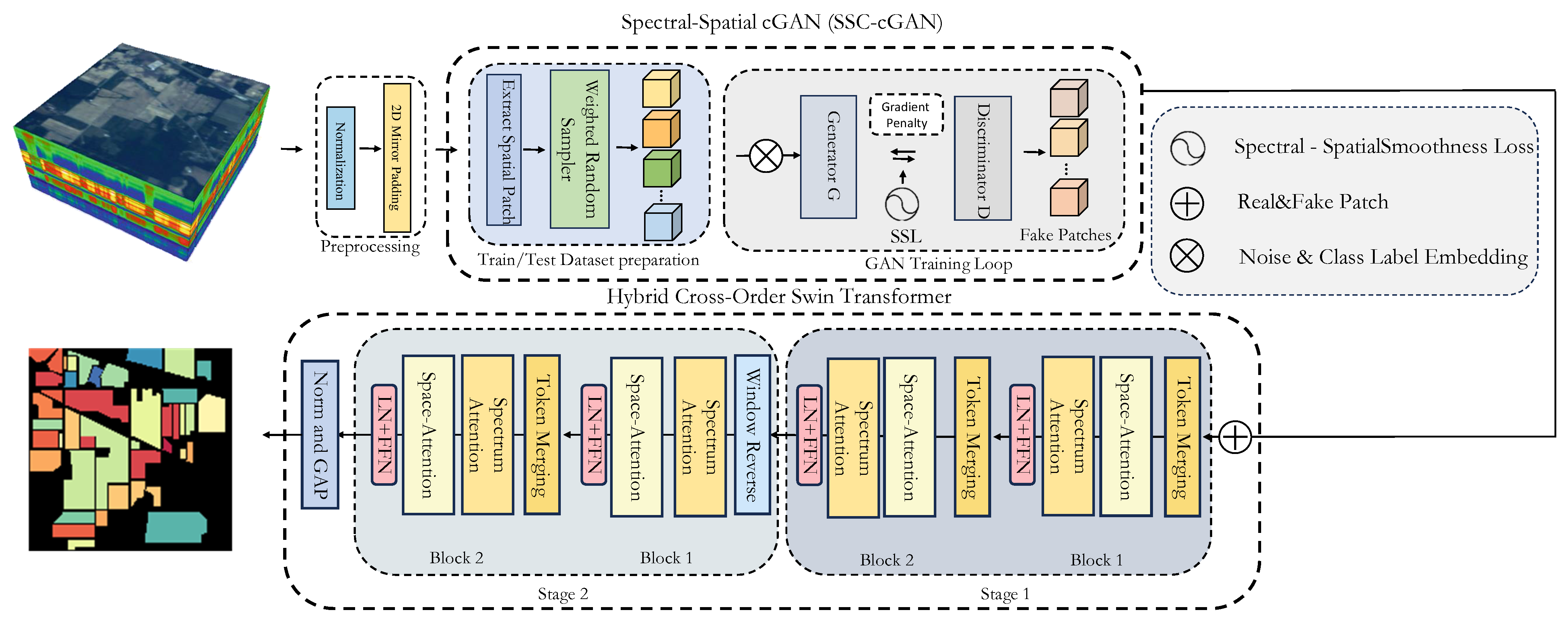
As illustrated in Figure 1, the overall architecture of S2A-Swin comprises three main components: a pre-processing module, an SSC-cGAN, and a HybridSwinBlock. Given a hyperspectral image (HSI) $\mathbf{I}\in {\mathbb{R}}^{H\times W\times C}$, where H, W, and C denote the height, width, and number of spectral bands, respectively, we first reshape $\mathbf{I}$ to ${\mathbf{I}}_{\mathrm{pn}}\in {\mathbb{R}}^{H^{\prime }\times W^{\prime }\times C}$ and apply normalization and zero-padding. An image patch $\mathbf{P}\in {\mathbb{R}}^{p\times p\times C}$, centred on the target pixel, is then cropped from ${\mathbf{I}}_{\mathrm{pn}}$ and fed into the SSC-cGAN, which generates a set of synthetic samples. The resulting embeddings are forwarded to the HybridSwinBlock, followed by a multilayer perceptron (MLP) that outputs the final prediction $\mathbf{Y}\in {\mathbb{R}}^{1\times N}$, where N is the number of classes. The network is trained end-to-end using the standard cross-entropy loss.

3.1. Data Preprocessing and Spatial-Spectral Patch Construction

In order to eliminate the negative impact of data scale differences in different spectral bands on model training, this study first performed normalization processing band by band. Hyperspectral images are usually represented as a three-dimensional data cube, and each pixel contains rich spectral information. The input hyperspectral image is represented as:

$$\mathbf{X}\in {\mathbb{R}}^{H\times W\times C},$$

where H and W are the image height and width, and C is the spectral dimension (number of bands). Let ${\mathbf{X}}_b$ ($b=1,2,\dots ,C$) denote the b-th spectral band; the normalised band ${\mathbf{X}}_b^{\mathrm{norm}}$ is defined by

$${\mathbf{x}}_b^{\mathrm{norm}}={\displaystyle \frac{x_b-min\left({\mathbf{X}}_b\right)}{max\left({\mathbf{X}}_b\right)-min\left({\mathbf{X}}_b\right)+\epsilon }},b=1,2,\dots ,C,$$

where $min\left({\mathbf{X}}_b\right)$ and $max\left({\mathbf{X}}_b\right)$ are, respectively, the minimum and maximum pixel values in band b, and $\epsilon ={10}^{-6}$ is a small constant that prevents division by zero.

To exploit spatial context, a square neighbourhood window of size $w\times w$ ($w=9$ in this study) is centred at every labelled pixel. For any pixel located at $(i,j)$ with a non-zero class label, the corresponding spatial–spectral patch ${\mathbf{P}}_{(i,j)}\in {\mathbb{R}}^{C\times w\times w}$ is constructed as

$${\mathbf{P}}_{(i,j)}={\mathbf{X}}^{\mathrm{norm}}\left[i-\delta :i+\delta ,j-\delta :j+\delta ,1:C\right],$$

where $\delta =\lfloor w/2\rfloor$ is the window radius ($\delta =4$ when $w=9$). To ensure that border pixels can provide a full spatial context, the normalised image ${\mathbf{X}}^{\mathrm{norm}}$ is mirror-padded along both spatial dimensions:

$${\mathbf{X}}_{\mathrm{pad}}=MirrorPad\left({\mathbf{X}}_{\mathrm{norm}},(\delta ,\delta )\right)$$

After padding, the spatial dimensions of ${\mathbf{X}}^{\mathrm{pad}}$ are extended from the original $H\times W$ to $(H+2\delta )\times (W+2\delta )$, which enables smooth extraction of patches near the image boundaries.

Each spatial–spectral patch ${\mathbf{P}}_{(i,j)}$ is paired with the class label $y_{(i,j)}$ of its centre pixel to form a supervised training sample:

$$({\mathbf{P}}_{(i,j)},y_{(i,j)}).$$

At the final stage of training and test split, we employ a stratified random sampling strategy to ensure that each class is well represented in both the training and test sets.

Let $N_c$ be the total number of available samples for class c, then the number of samples selected for the test set, $N_c^{\mathrm{test}}$, is defined as:

$$N_c^{\mathrm{test}}=max\left(⌊\gamma ·N_c⌋,1\right),0<\gamma <1,$$

where $\gamma$ is the proportion of test samples. In this study, we set $\gamma =0.9$ to ensure that each class has at least one sample in the test set, while the remaining samples are used for training.

3.2. Spectral–Spatial GAN (SSC-cGAN)

The goal of SSC-cGAN is to generate sample patches that closely resemble hyperspectral characteristics under conditions of data imbalance and sample scarcity, thereby augmenting the training dataset. During training, we first perform one or more gradient descent steps on the generator G, followed by gradient updates on the discriminator D. To enhance model stability and generation quality, a gradient penalty term is introduced, which is computed by sampling random points between real and generated patches through interpolation. Throughout the iterative training process, the discriminator D learns to distinguish between real patches and generated ones conditioned on class labels, while the generator G progressively improves to produce increasingly realistic patches. These generated patches become indistinguishable from real ones and adhere to spectral and spatial smoothness constraints. Once training converges, we use G to generate a large number of synthetic patches for each class, augmenting the original training set. In the subsequent classification model training, we combine real and synthetic samples. In cases where certain classes have very few samples, the synthetic data significantly increases the size and diversity of the training dataset. To ensure balanced representation across classes, we apply a class-balanced sampling strategy during augmentation. The detailed implementation of each module is described below:

3.2.1. Generative Adversarial Backbone

We adopt Conditional WGAN-GP (Wasserstein GAN with Gradient Penalty) to generate synthetic hyperspectral images (HSI) for spectral augmentation. The WGAN-GP consists of two convolutional neural networks: a generator G and a discriminator D. The generator $G\left(z\right|y)$ takes as input a random noise vector z (sampled from a uniform or Gaussian distribution) and a conditional label y, and outputs a synthetic hyperspectral image $\widehat{X}=G\left(z\right|y)\in {\mathbb{R}}^{P\times P\times B}$. The generator is implemented as a deep convolutional network. It upsamples the noise into an image with $P\times P$ pixels and B spectral bands, using transposed convolutions (deconvolution) or pixel-shuffling techniques. The conditional label y is embedded and injected into intermediate layers via conditional normalization. The discriminator $D\left(X\right|y)$ is also a convolutional network. It takes as input either a real or synthetic HSI X, together with the label y, and outputs a scalar score. Unlike conventional GANs, which use binary cross-entropy loss, WGAN-GP employs the Earth-Mover (Wasserstein) distance to measure the discrepancy between the real and generated distributions. The discriminator (also referred to as the critic) does not output probabilities, but rather estimates the Wasserstein distance by maximizing the difference between real and generated samples. In practice, the training objective minimizes the negative critic score with the addition of a gradient penalty term for regularization. Formally, let $D\left(X\right|y)$ denote the critic’s output score for an input HSI X with label y. The discriminator loss is defined as:

$$\begin{array}{cc}\hfill L_D& =-{\mathbb{E}}_{X_{\mathrm{real}}\sim p_{\mathrm{data}}}\left[D\left(X_{\mathrm{real}}\right|y)\right]\hfill \\ & +{\mathbb{E}}_{z\sim p\left(z\right)}\left[D\left(G\right(z\left|y\right)\left|y\right)\right]\hfill \\ \hfill & +{\lambda }_{GP}{\mathbb{E}}_{\widehat{X}}\left[{\left({\parallel {\nabla }_{\widehat{X}}D\left(\widehat{X}\right|y)\parallel }_2-1\right)}^2\right].\hfill \end{array}$$

(1)

where the first term $-{\mathbb{E}}_{x\sim p_{\mathrm{real}}}\left[D(x\mid y)\right]$ encourages the discriminator D to assign higher scores to real patches, and the second term ${\mathbb{E}}_{z\sim p\left(z\right)}\left[D(G(z\mid y)\mid y)\right]$ encourages D to assign lower scores to generated patches. The third term is the gradient penalty proposed in WGAN-GP (weighted by ${\lambda }_{\mathrm{GP}}$), where $\widehat{x}$ denotes samples interpolated between real and generated patches (i.e., for a random $ϵ\in [0,1]$, $\widehat{x}=ϵx+(1-ϵ)\tilde{x}$). This term penalizes the gradient norm $\parallel {\nabla }_{\widehat{x}}D(\widehat{x}\mid y){\parallel }_2$ to be close to 1, thereby enforcing the Lipschitz constraint required for Wasserstein distance estimation. The gradient penalty helps stabilize training and prevents the discriminator from becoming too sharp or discontinuous, which is especially important for high-dimensional HSI input spaces.

The generator aims to fool the discriminator while adhering to spectral smoothness regularization. Specifically, the generator G tries to maximize $D\left(G\right(z\mid y)\mid y)$ (i.e., the discriminator’s score for fake data), as a higher score implies that the discriminator considers the fake data more realistic. Therefore, we minimize the negative of this score. Without regularization, the basic generator loss would be:

$$L_{G,\mathrm{adv}}=-{\mathbb{E}}_{z\sim p\left(z\right)}\left[D(G(z\mid y)\mid y)\right]$$

3.2.2. Spectral–Spatial Smoothness Constraint (SSC)

The continuity of hyperspectral data arises inherently from the continuous spectral reflectance properties of real-world materials and is further modulated by the overlapping Spectral Response Functions (SRFs) of adjacent detector elements in the spectrometer. While natural hyperspectral signals may exhibit low-frequency variations due to atmospheric scattering, the synthetic samples generated by unconstrained GANs often suffer from unphysical high-frequency spectral jitter. This jitter is akin to amplified sensor shot noise or adversarial checkerboard artifacts, which do not conform to physical imaging mechanisms. However, the existing data augmentation methods based on generative adversarial networks (GANs) do not explicitly consider this physical continuity constraint along the spectral dimension, which often leads to drastic unphysical changes between bands or unrealistic spectral anomalies. To this end, we propose an explicit spectral smoothness constraint mechanism (Spectral Smoothness Constraint, SSC). The core idea is to explicitly introduce the band continuity of hyperspectral data as a regularization term into the optimization process of the generative network. Therefore, we express this spectral continuity feature as:

$$x_{c+1}(i,j)\approx x_c(i,j),c=1,2,\dots ,C-1,$$

(2)

where $x_c(i,j)$ denotes the pixel value at spatial location $(i,j)$ in band c of a real sample. Guided by this observation, we enforce an analogous continuity on the generated samples,

$${\widehat{x}}_{c+1}(i,j)\approx {\widehat{x}}_c(i,j),c=1,2,\dots ,C-1,$$

(3)

where $\widehat{x}=G(z,y)$ is the output of the generator G given latent code z (and, if applicable, conditioning y). Equivalently,

$${\left[G(z,y)\right]}_{c+1}(i,j)\approx {\left[G(z,y)\right]}_c(i,j),c=1,2,\dots ,C-1.$$

(4)

Specifically, the proposed SSC penalizes discrepancies between adjacent spectral bands of a generated sample, thereby enforcing realistic and smooth behavior along the spectral dimension. To rigorously encode this continuity, we design a loss that directly measures inter-band differences and adopt the squared Euclidean distance so that abrupt changes are strongly penalized. The spectral smoothness loss is defined as

$${\mathcal{L}}_{\mathrm{spec}}={\mathbb{E}}_{z,y}\left[{\displaystyle \frac{1}{C-1}}\sum _{c=1}^{C-1}{∥G{(z,y)}_{c+1}-G{(z,y)}_c∥}_2^2\right],$$

(5)

where ${\mathcal{L}}_{\mathrm{spec}}$ denotes the spectral smoothness regularization term, $G(z,y)$ is the generator’s hyperspectral output, and C is the number of spectral bands. Here $G{(z,y)}_c\in {\mathbb{R}}^{H\times W}$ is the image at band c, and ${\parallel ·\parallel }_2^2$ denotes the squared ${\ell }_2$ norm over spatial pixels, i.e.,

$${∥G{(z,y)}_{c+1}-G{(z,y)}_c∥}_2^2=\sum _{i=1}^H\sum _{j=1}^W{\left(G{(z,y)}_{c+1}(i,j)-G{(z,y)}_c(i,j)\right)}^2.$$

(6)

Abrupt discrepancies between adjacent spectral bands are typically physically implausible and often indicate anomalies or noise. Therefore, by explicitly penalizing such discrepancies, we can effectively reduce the probability that the generator produces anomalous samples. This explicit constraint drives the generator to directly learn, during training, to produce spectra that are smoother and more consistent with real-world material characteristics, thereby markedly improving the quality of synthetic samples. In addition, to further enhance the quality of the generated data, we introduce an auxiliary spatial smoothness regularization to suppress abrupt spatial changes in the generated samples:

$$\begin{array}{cc}\hfill {\mathcal{L}}_{\mathrm{spat}}=& {\mathbb{E}}_{z,y}[{\displaystyle \frac{1}{C(w-1)w}}\sum _{i=1}^{w-1}\sum _{j=1}^w{∥G{(z,y)}_{:,i+1,j}-G{(z,y)}_{:,i,j}∥}_2^2\hfill \\ \hfill & +{\displaystyle \frac{1}{Cw(w-1)}}\sum _{i=1}^w\sum _{j=1}^{w-1}{∥G{(z,y)}_{:,i,j+1}-G{(z,y)}_{:,i,j}∥}_2^2].\hfill \end{array}$$

(7)

The spatial smoothness loss enforces local spatial continuity of generated data, preventing spatial artifacts or anomalous patterns. Serving as an auxiliary term, it cooperates with the spectral smoothness regularization to jointly improve data quality along both the spatial and spectral dimensions. The final optimization objective of the generator combines the adversarial loss with the above constraints:

$${\mathcal{L}}_G={\mathcal{L}}_{G,\mathrm{adv}}+{\alpha }_{\mathrm{spec}}{\mathcal{L}}_{\mathrm{spec}}+{\alpha }_{\mathrm{spat}}{\mathcal{L}}_{\mathrm{spat}}.$$

(8)

Unlike conventional methods that encourage band-to-band continuity only implicitly, our approach encodes an explicit difference loss between adjacent spectral bands directly in the optimization objective, thereby enabling precise control over the generated data. A potential concern regarding the SSC is whether enforcing local smoothness might inadvertently blur the discriminative features of the synthesized samples, such as specific absorption valleys or red-edge characteristics crucial for classification. It is important to emphasize that SSC does not operate in isolation. In the overall objective (Equation (8)), the spectral smoothness is balanced by the conditional adversarial loss ${\mathcal{L}}_{G,adv}$. The conditional discriminator rigorously enforces the preservation of class-specific spectral signatures to prevent mode mixing. Consequently, controlled by an appropriate weight ${\alpha }_{spec}$, the SSC functions as a localized physical low-pass filter: it effectively mitigates unphysical inter-band high-frequency noise without over-smoothing the macro-level spectral discriminative features (e.g., absorption depths) that are essential for accurate representation and classification.

3.3. HybridSwinBlock

Traditional Swin Transformer usually only performs window division and attention calculation in the spatial dimension, ignoring the importance of the spectral dimension and its interaction with the spatial dimension [35]. To this end, this study proposes the HybridSwinBlock module: it integrates the spatial window mechanism and the spectral window mechanism. By completing the window division and attention calculation of the spatial and spectral dimensions in sequence within a single block, and at the same time, alternating between the spatial and spectral dimensions, it can achieve a deep fusion of spatial and spectral features, and more fully capture the interaction between spatial and spectral features in hyperspectral images. The specific process and data changes are as follows:

A hyperspectral image is typically represented as a three-dimensional data cube, where each pixel contains rich spectral information. The input hyperspectral image is denoted by

$$X\in {\mathbb{R}}^{h\times w\times c},$$

(9)

where h and w are the image height and width, and c is the spectral dimension (number of channels). We first partition the spatial plane into non-overlapping windows of size $w_{\mathrm{spatial}}\times w_{\mathrm{spatial}}$. Within each window, the data has shape $C\times w_{\mathrm{spatial}}\times w_{\mathrm{spatial}}$, and the collection of windowed tensors is

$$X_{\mathrm{windows}}\in {\mathbb{R}}^{N_{\mathrm{win}}\times C\times w_{\mathrm{spatial}}\times w_{\mathrm{spatial}}},$$

(10)

where

$$N_{\mathrm{win}}={\displaystyle \frac{H}{w_{\mathrm{spatial}}}}\times {\displaystyle \frac{W}{w_{\mathrm{spatial}}}}$$

(11)

is the total number of spatial windows after partitioning. For efficient attention computation, the data inside each window is flattened into a two-dimensional matrix of size $\left(w_{\mathrm{spatial}}^2\right)\times C$, and a multi-head self-attention (MSA) operation is applied to extract spatial features. After the spatial attention, the features of each window are reshaped back to $C\times w_{\mathrm{spatial}}\times w_{\mathrm{spatial}}$ and reassembled to the full feature map of size $C\times H\times W$:

$$X_{\mathrm{spatial}}=\mathrm{Spatial-MSA}\left(\mathrm{WindowPartition}\left(X,w_{\mathrm{spatial}}\right)\right).$$

(12)

After obtaining $X_{\mathrm{spatial}}$, its dimensionality remains $C\times H\times W$. No further reshaping is performed; the spatially attended features are directly used as the input to the spectral-attention computation:

$$X_{\mathrm{intermediate}}=X_{\mathrm{spatial}}.$$

(13)

Along the spectral dimension, $X_{\mathrm{intermediate}}$ is partitioned into contiguous spectral windows of size $w_{\mathrm{spectral}}$. Each window then has shape $w_{\mathrm{spectral}}\times H\times W$. Next, the data in each spectral window is flattened into a two-dimensional matrix of size $(H\times W)\times w_{\mathrm{spectral}}$, and a multi-head self-attention operation is performed independently within every window along the spectral dimension to capture inter-band dependencies and spectral continuity. After spectral attention, the features are reshaped back to $C\times H\times W$:

$$X_{\mathrm{spectral}}=\mathrm{Spectral-MSA}\left(\mathrm{SpectralPartition}\left(X_{\mathrm{intermediate}},w_{\mathrm{spectral}}\right)\right).$$

(14)

The final output feature representation is

$$X_{\mathrm{out}}=X_{\mathrm{spectral}}.$$

(15)

To further enhance the network’s ability to capture fine-grained spatial and spectral features, we propose an interleaved ordering mechanism inside each HybridSwinBlock, in which consecutive blocks adopt different window-attention orders:

Apply spatial attention first, followed by spectral attention:

$$X_{\mathrm{out}}=\mathrm{Spectral-MSA}\left(\mathrm{Spatial-MSA}\left(X\right)\right).$$

(16)

Apply spectral attention first, followed by spatial attention:

$$X_{\mathrm{out}}=\mathrm{Spatial-MSA}\left(\mathrm{Spectral-MSA}\left(X\right)\right).$$

(17)

Multiple HybridSwinBlocks together form a SwinStage. Each SwinStage consists of a series of HybridSwinBlocks; adjacent blocks alternate between the spatial-first and spectral-first windowing orders. That is, if the n-th block is spatial-first, then the $(n+1)$-th block is spectral-first. This interleaved attention computation enables the model to capture richer spectral interactions present in HSI data. The hybrid Swin Transformer effectively balances model complexity with hyperspectral-specific feature learning. By restricting spatial self-attention to local windows, we keep the computational cost within a controllable range (per layer $𝒪\left(P^2{M}^2\right)$, rather than the $𝒪\left({\left(P^2\right)}^2\right)$ of global attention). Moreover, spectral attention is inherently parallel across spatial locations because the spectral interactions of each pixel are computed independently, which allows an efficient GPU implementation with minimal inter-thread communication.

The alternation of spatial and spectral self-attention yields a hybrid multi-scale attention mechanism, enabling tokens to progressively integrate spatial neighborhood context together with inter-spectral dependencies as depth increases. Compared with traditional hybrid spatial–spectral filtering methods, our approach learns a dynamically weighted mixture (attention) instead of fixed convolutional kernels, thereby capturing more flexible, data-driven relationships more efficiently.

4. Experiments

In this section, we describe the dataset in Section 4.1, and then describe the evaluation metrics and implementation details in Section 4.2. To evaluate our S2A-Swin, we present and discuss the quantitative and qualitative results, as well as analyze the computational complexity of different methods, in Section 4.3.

4.1. Datasets

• Indian Pines dataset:

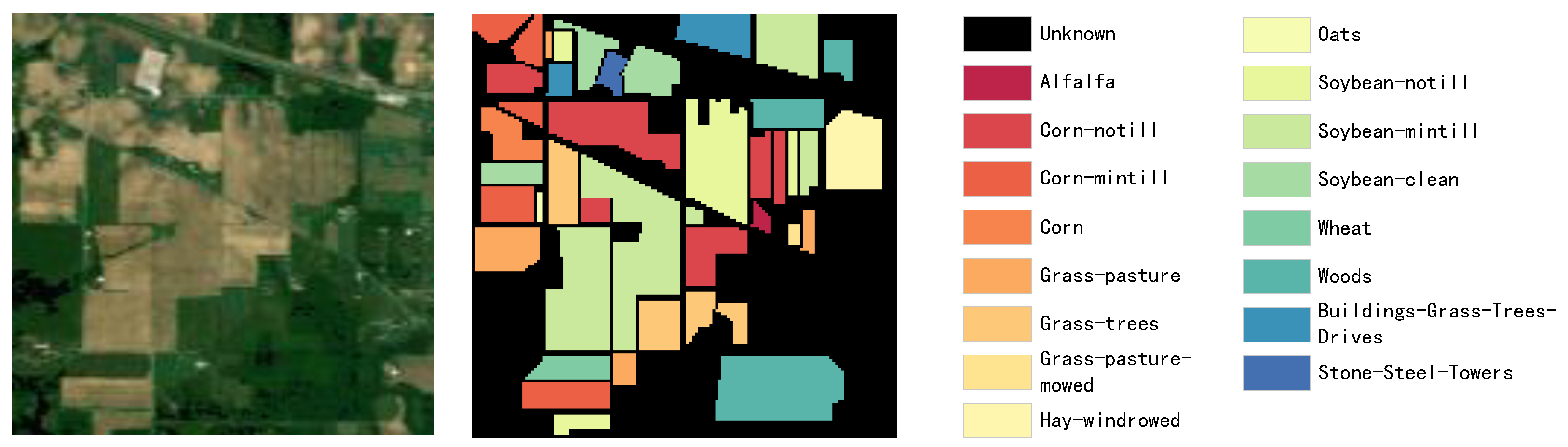
The Indian Pines dataset was collected in 1992 over northwestern Indiana (USA) by the Airborne Visible/Infrared Imaging Spectrometer (AVIRIS). It contains an image of size $145\times 145$ pixels with 224 spectral reflectance bands spanning wavelengths from $0.4\times {10}^{-6}$ to $2.5\times {10}^{-6}\mathrm{m}$. After removing bands covering atmospheric absorption regions [104–108], [150–163], and [220–224], the data are reduced to 200 bands. The scene comprises roughly two-thirds agricultural fields and one-third forest or other natural perennial vegetation. Land cover is divided into 16 classes, e.g., soybeans (min-till), and corn (min-till) as shown in Figure 2, with the number of samples for each class listed in Table 1.

• University of Pavia dataset:

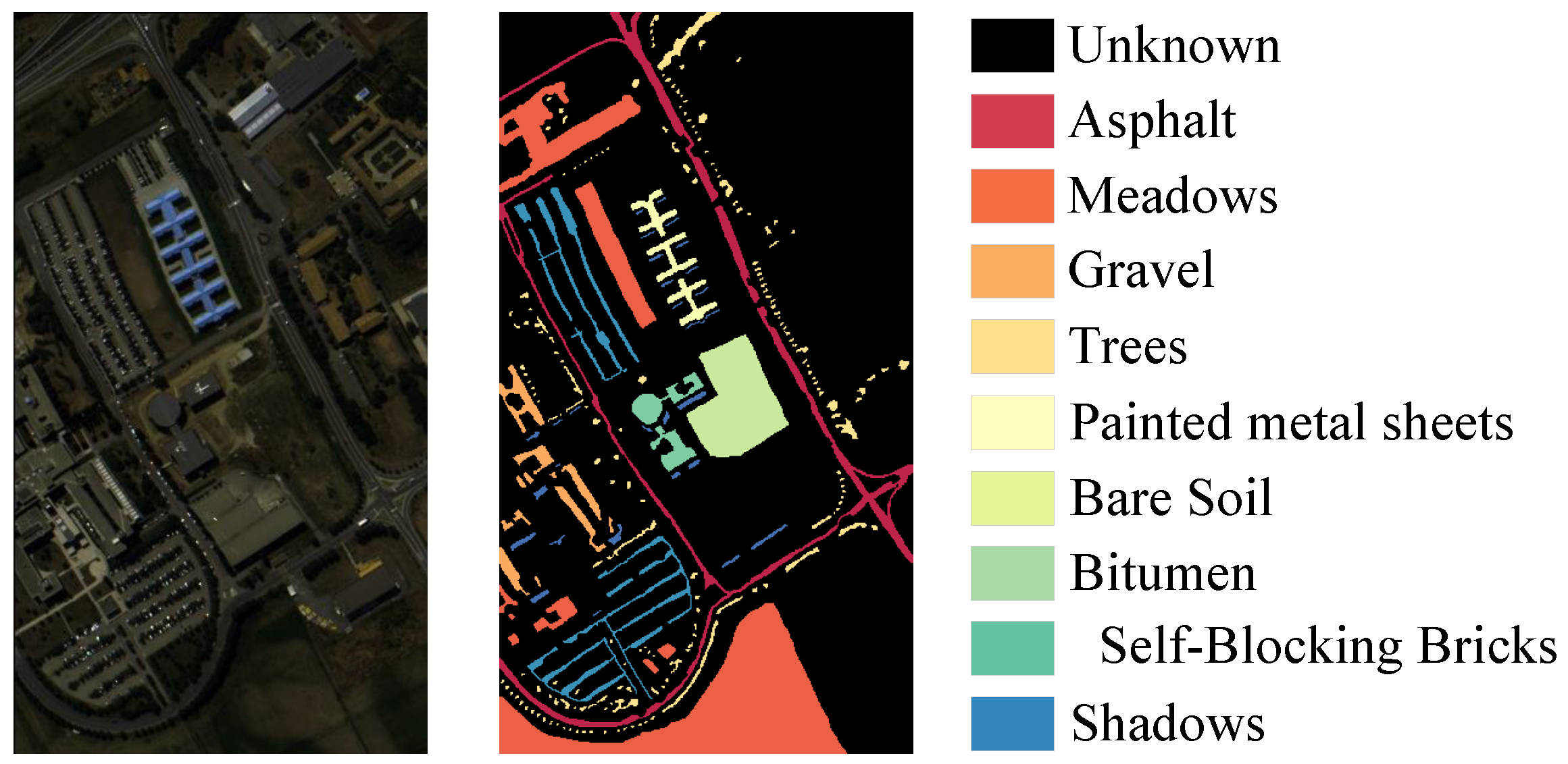
Provided by the Telecommunications and Remote Sensing Laboratory of the University of Pavia, this dataset was acquired over northern Pavia (Italy) during an airborne flight campaign using the Reflective Optics System Imaging Spectrometer (ROSIS). The image has size $610\times 340$ pixels with 103 spectral bands and is labeled into 9 categories, including asphalt, meadows, gravel, trees, painted metal sheets, bare soil, bitumen, self-blocking bricks, and shadows.as shown in Figure 3, with the number of samples for each class listed in Table 2.

• Salinas Scene dataset:

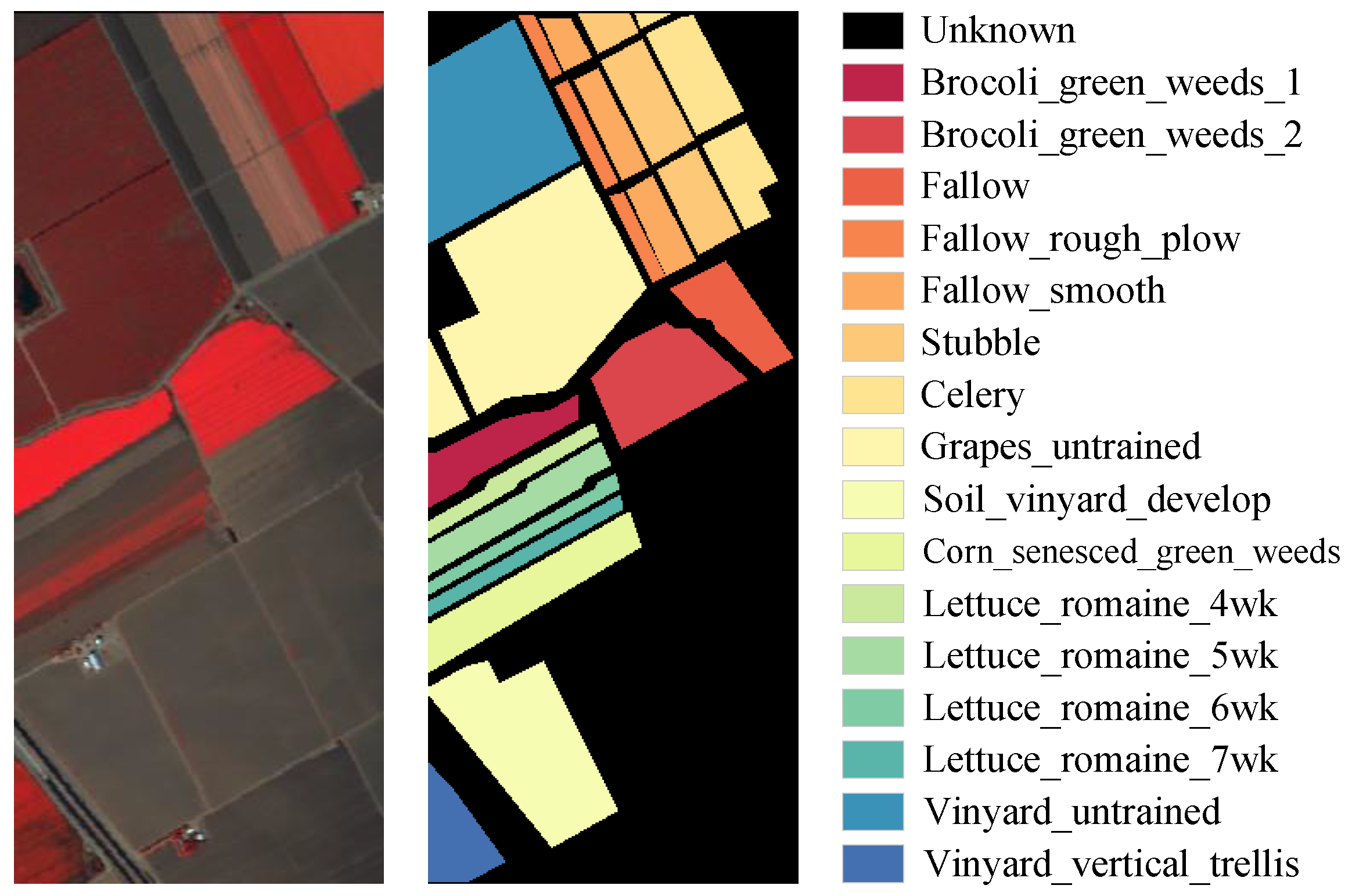
The Salinas Scene dataset was collected by AVIRIS over California’s Salinas Valley with 224 spectral bands and a high spatial resolution of $3.7\mathrm{m}$ per pixel. It contains 16 classes, such as Fallow, Stubble, and Celery in Figure 4. Table 3 reports the distribution of training and test samples for these datasets.

• BOS Dataset:

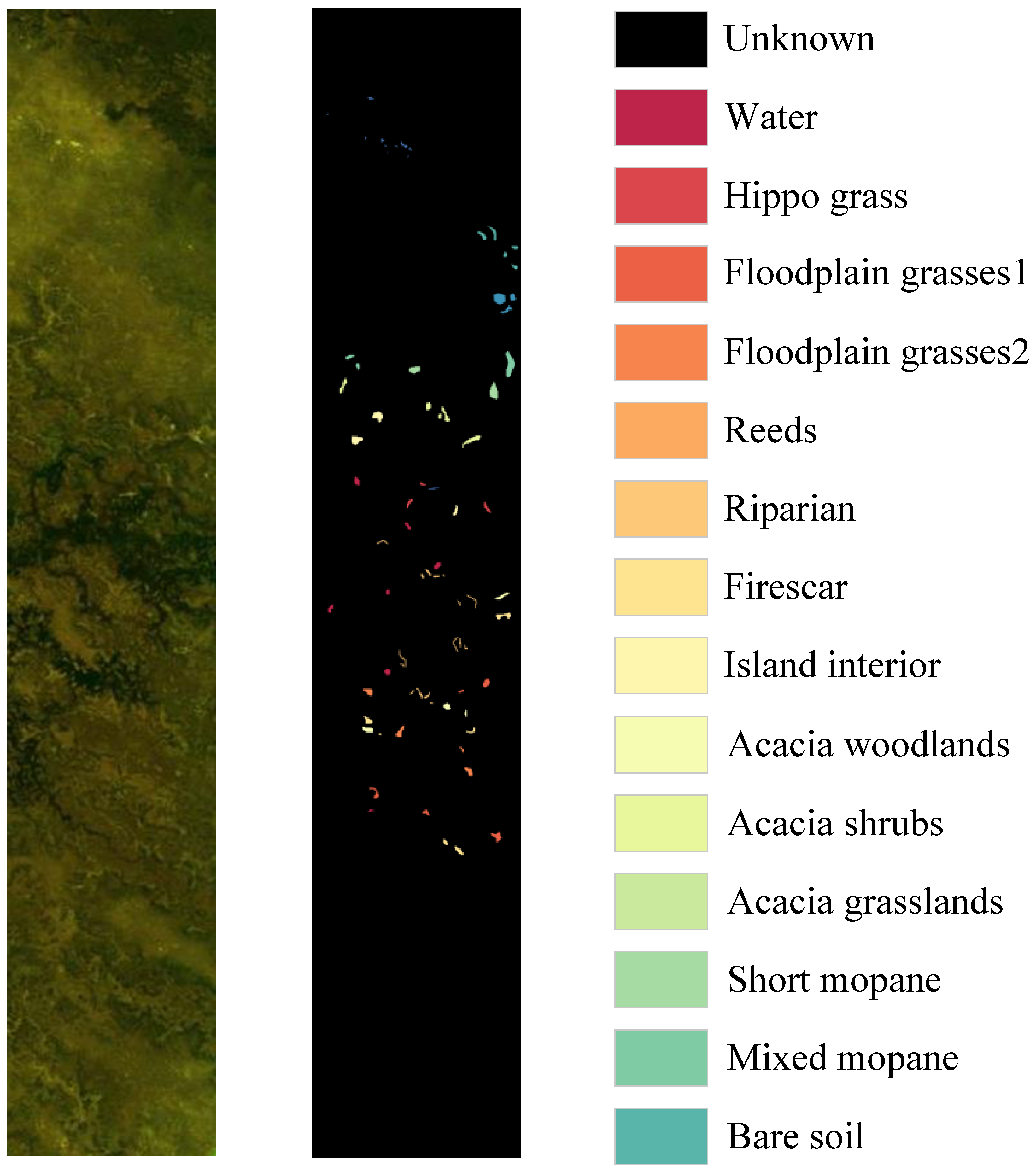
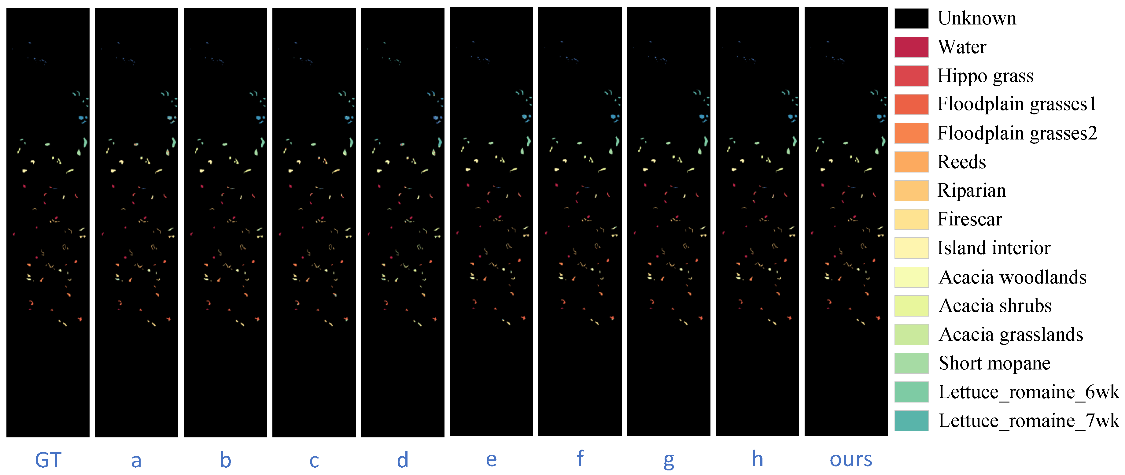
BOS Dataset was acquired by NASA EO-1 satellite over the Okavango Delta in BOS from 2001 to 2004. The Hyperion sensor on EO-1 captures data at a 30 m pixel resolution across a 7.7 km strip in 242 bands spanning the 400–2500 nm range with 10 nm spectral windows. The UT Center for Space Research performed data preprocessing to mitigate the effects of faulty detectors, inter-detector miscalibration, and intermittent anomalies. The ground truth provides sixteen different land-cover classes, as shown in Figure 5, with the number of samples for each class listed in Table 4. The wavelength information was obtained from the EO-1 data meta files available through Portal Gscloud.

Figure 3. Illustration of the PU dataset. The pseudocolor image is displayed on the left, and the corresponding ground-truth land-cover map is shown on the right, where each color represents a specific land-cover category.

Figure 3. Illustration of the PU dataset. The pseudocolor image is displayed on the left, and the corresponding ground-truth land-cover map is shown on the right, where each color represents a specific land-cover category.

Figure 4. Illustration of the SA dataset. The pseudocolor image is displayed on the left, and the corresponding ground-truth land-cover map is shown on the right, where each color represents a specific land-cover category.

Figure 4. Illustration of the SA dataset. The pseudocolor image is displayed on the left, and the corresponding ground-truth land-cover map is shown on the right, where each color represents a specific land-cover category.

Table 1. The detailed information of IP dataset.

No.	Class Name	Training Samples	Test Samples	Total Samples
1	Alfalfa	5	41	46
2	Corn-notill	143	1285	1428
3	Corn-min	83	747	830
4	Corn	24	213	237
5	Grass-pasture	49	434	483
6	Grass-trees	73	657	730
7	Grass-pasture-mowed	3	25	28
8	Hay-windrowed	48	430	478
9	Oats	2	18	20
10	Soybean-notill	98	874	972
11	Soybean-mintill	246	2209	2455
12	Soybean-clean	60	533	593
13	Wheat	21	184	205
14	Woods	127	1138	1265
15	Buildings-Grass-Trees	39	347	386
16	Stone-Steel-Towers	10	83	93
Total		1031	9218	10,249

Table 1. The detailed information of IP dataset.

No.	Class Name	Training Samples	Test Samples	Total Samples
1	Alfalfa	5	41	46
2	Corn-notill	143	1285	1428
3	Corn-min	83	747	830
4	Corn	24	213	237
5	Grass-pasture	49	434	483
6	Grass-trees	73	657	730
7	Grass-pasture-mowed	3	25	28
8	Hay-windrowed	48	430	478
9	Oats	2	18	20
10	Soybean-notill	98	874	972
11	Soybean-mintill	246	2209	2455
12	Soybean-clean	60	533	593
13	Wheat	21	184	205
14	Woods	127	1138	1265
15	Buildings-Grass-Trees	39	347	386
16	Stone-Steel-Towers	10	83	93
Total		1031	9218	10,249

Figure 5. Illustration of the BOS dataset. The pseudocolor image is displayed on the left, and the corresponding ground-truth land-cover map is shown on the right, where each color represents a specific land-cover category.

Figure 5. Illustration of the BOS dataset. The pseudocolor image is displayed on the left, and the corresponding ground-truth land-cover map is shown on the right, where each color represents a specific land-cover category.

Table 2. The detailed information of PU dataset.

No.	Class Name	Training Samples	Test Samples	Total Samples
1	Asphalt	663	5968	6631
2	Meadows	1864	16,785	18,649
3	Gravel	209	1890	2099
4	Trees	306	2758	3064
5	Painted metal sheets	134	1211	1345
6	Bare Soil	502	4527	5029
7	Bitumen	133	1197	1330
8	Self-Blocking Bricks	368	3314	3682
9	Shadows	94	853	947
Total		4273	38,503	42,776

Table 2. The detailed information of PU dataset.

No.	Class Name	Training Samples	Test Samples	Total Samples
1	Asphalt	663	5968	6631
2	Meadows	1864	16,785	18,649
3	Gravel	209	1890	2099
4	Trees	306	2758	3064
5	Painted metal sheets	134	1211	1345
6	Bare Soil	502	4527	5029
7	Bitumen	133	1197	1330
8	Self-Blocking Bricks	368	3314	3682
9	Shadows	94	853	947
Total		4273	38,503	42,776

Table 3. The detailed information of SA dataset.

No.	Class Name	Training Samples	Test Samples	Total Samples
1	Broccoli-green-weeds-1	200	1809	2009
2	Broccoli-green-weeds-2	372	3354	3726
3	Fallow	197	1779	1976
4	Fallow-rough-plow	139	1255	1394
5	Fallow-smooth	267	2411	2678
6	Stubble	395	3564	3959
7	Celery	357	3222	3579
8	Grapes-untrained	1127	10,144	11,271
9	Soil-vineyard-develop	620	5583	6203
10	Corn-senesced-green-weeds	327	2951	3278
11	Lettuce-romaine-4wk	106	962	1068
12	Lettuce-romaine-5wk	192	1735	1927
13	Lettuce-romaine-6wk	91	825	916
14	Lettuce-romaine-7wk	107	963	1070
15	Vineyard-untrained	726	6542	7268
16	Vineyard-vertical-trellis	180	1627	1807
Total		5403	48,726	54,129

Table 3. The detailed information of SA dataset.

No.	Class Name	Training Samples	Test Samples	Total Samples
1	Broccoli-green-weeds-1	200	1809	2009
2	Broccoli-green-weeds-2	372	3354	3726
3	Fallow	197	1779	1976
4	Fallow-rough-plow	139	1255	1394
5	Fallow-smooth	267	2411	2678
6	Stubble	395	3564	3959
7	Celery	357	3222	3579
8	Grapes-untrained	1127	10,144	11,271
9	Soil-vineyard-develop	620	5583	6203
10	Corn-senesced-green-weeds	327	2951	3278
11	Lettuce-romaine-4wk	106	962	1068
12	Lettuce-romaine-5wk	192	1735	1927
13	Lettuce-romaine-6wk	91	825	916
14	Lettuce-romaine-7wk	107	963	1070
15	Vineyard-untrained	726	6542	7268
16	Vineyard-vertical-trellis	180	1627	1807
Total		5403	48,726	54,129

Table 4. The detailed information of BOS dataset.

No.	Class Name	Training Samples	Test Samples	Total Samples
1	Water	27	243	270
2	Hippo grass	11	90	101
3	Floodplain grasses 1	26	225	251
4	Floodplain grasses 2	22	193	215
5	Reeds	27	242	269
6	Riparian	27	242	269
7	Firescar	26	233	259
8	Island interior	21	182	203
9	Acacia woodlands	32	282	314
10	Acacia shrubs	25	223	248
11	Acacia grasslands	31	274	305
12	Short mopane	19	162	181
13	Mixed mopane	27	241	268
14	Bare soil	10	85	95
Total		331	2917	3248

Table 4. The detailed information of BOS dataset.

No.	Class Name	Training Samples	Test Samples	Total Samples
1	Water	27	243	270
2	Hippo grass	11	90	101
3	Floodplain grasses 1	26	225	251
4	Floodplain grasses 2	22	193	215
5	Reeds	27	242	269
6	Riparian	27	242	269
7	Firescar	26	233	259
8	Island interior	21	182	203
9	Acacia woodlands	32	282	314
10	Acacia shrubs	25	223	248
11	Acacia grasslands	31	274	305
12	Short mopane	19	162	181
13	Mixed mopane	27	241	268
14	Bare soil	10	85	95
Total		331	2917	3248

4.2. Experimental Setup and Performance Evaluation Metrics

4.2.1. Experimental Setup

To ensure the effectiveness and superiority of the proposed method and comprehensively and fairly evaluate our method on the four datasets, we use three key indicators, AA (indicating the proportion of correctly classified samples of all categories), OA (indicating the average classification accuracy of each category), and Kappa coefficient, to comprehensively evaluate the algorithm and conduct quantitative analysis of different methods.

4.2.2. Evaluation Indexes

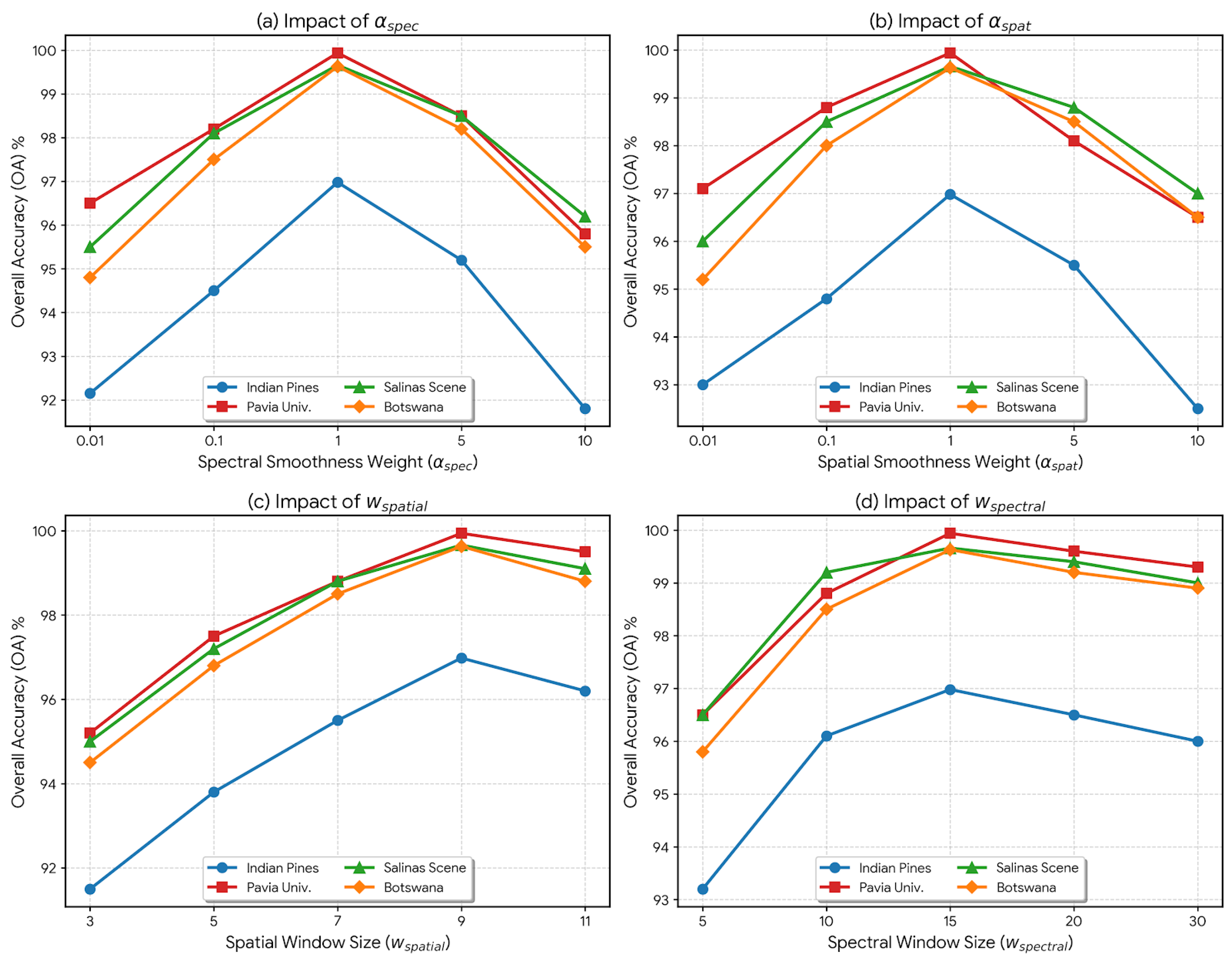
For all four datasets, we adopt a unified configuration for S2A-Swin. The multi-head self-attention layers use four heads ($h=4$), and the hidden size of each MLP layer is set to eight times the input dimension. In the SSC-cGAN module, the noise vector dimension is set to 100, with a gradient-penalty coefficient of ${\lambda }_{\mathrm{GP}}=10$ and a critic–generator update ratio of $n_{\mathrm{critic}}=5$. All classifiers are trained with the Adam optimizer with an initial learning rate of $1\times {10}^{-3}$ and a fixed weight decay of $1\times {10}^{-4}$; the learning rate (not the weight decay) is multiplied by 0.9 every 100 epochs. All experiments are conducted on a server equipped with an NVIDIA GTX 5090D GPU (32 GB). Furthermore, the selection of key spatial–spectral hyperparameters is rigorously justified through a parameter sensitivity analysis (illustrated in Figure 6). We observe an inverted-U performance trend for the smoothness regularization weights (${\alpha }_{spec}$ and ${\alpha }_{spat}$); excessively small values fail to suppress unphysical high-frequency GAN artifacts, while overly large values over-smooth critical discriminative features and spatial boundaries. Consequently, both ${\alpha }_{spec}$ and ${\alpha }_{spat}$ are optimally set to 1.0. Similarly, increasing the spatial window size initially improves accuracy by capturing richer local geometry, but sizes beyond 9 begin to introduce heterogeneous noise from adjacent classes. Therefore, we extract $9\times 9$ spatial patches centred at each labeled pixel ($w_{spatial}=9$), and dynamically set the spectral window size ($w_{spectral}$) around 10 to 15 to optimally balance long-range spectral dependency modeling with computational efficiency.

4.3. Experimental Result and Analysis

4.3.1. Quantitative Analysis

Based on the quantitative results in

Table 5. Classification results of different methods using 10% training samples per class on IP dataset.

Classes	SVM [8]	1DCNN [36]	3DCNN [37]	VIT [38]	HSIC-FM [39]	CSIL [40]	SWIN [28]	CLOLN [41]	Ours
1	67.34%	47.83%	57.60%	53.25%	61.90%	95.24%	50.00%	100.00%	95.12%
2	67.86%	42.35%	68.90%	66.20%	70.33%	90.67%	76.54%	61.91%	94.71%
3	93.48%	60.87%	66.10%	86.41%	60.31%	89.42%	78.09%	99.60%	96.92%
4	94.63%	89.49%	53.60%	89.71%	45.79%	84.11%	85.23%	98.96%	92.02%
5	88.52%	92.40%	76.50%	87.66%	77.47%	90.57%	52.59%	100.00%	96.08%
6	94.76%	97.04%	93.60%	89.98%	94.37%	96.19%	90.07%	100.00%	95.13%
7	73.86%	59.69%	63.50%	72.22%	15.38%	73.08%	92.86%	100.00%	88.00%
8	52.07%	65.38%	95.40%	66.00%	98.96%	100.00%	96.86%	95.98%	100.00%
9	72.70%	93.44%	94.70%	57.09%	58.33%	27.78%	100.00%	100.00%	94.44%
10	98.77%	99.38%	70.70%	97.53%	68.06%	91.20%	87.32%	97.47%	94.51%
11	81.67%	84.00%	77.00%	87.62%	76.09%	96.65%	83.64%	99.94%	98.60%
12	71.82%	86.06%	52.50%	63.94%	53.93%	91.95%	73.79%	99.81%	96.06%
13	95.56%	91.11%	87.10%	95.56%	98.65%	100.00%	96.37%	99.03%	100.00%
14	82.05%	84.62%	92.10%	79.49%	93.11%	95.79%	96.77%	96.78%	99.82%
15	90.91%	100.00%	56.70%	90.91%	64.94%	93.97%	72.82%	93.89%	96.83%
16	100.00%	80.00%	60.00%	80.00%	97.62%	100.00%	80.14%	91.18%	97.59%
OA	72.36%	70.43%	74.47%	71.86%	75.76%	93.67%	83.05%	90.19%	96.98%
AA	83.16%	79.60%	70.47%	78.97%	70.95%	88.54%	78.75%	95.91%	95.99%
Kappa	68.88%	66.42%	70.90%	68.04%	72.28%	92.79%	78.05%	88.88%	96.56%

,

Table 6. Classification results of different methods using 5% training samples per class on IP dataset.

Classes	SVM [8]	1DCNN [36]	3DCNN [37]	VIT [38]	HSIC-FM [39]	CSIL [40]	SWIN [28]	CLOLN [41]	Ours
OA	60.31%	63.53%	64.30%	62.86%	69.50%	86.25%	73.85%	82.55%	89.91%
AA	64.16%	65.60%	61.90%	69.97%	64.20%	85.64%	66.32%	85.63%	90.30%
Kappa	58.88%	66.42%	60.18%	67.85%	65.10%	84.50%	68.90%	80.10%	90.40%

,

Table 7. Classification results of different methods using 5% training samples per class on BOS dataset.

Classes	SVM [8]	1DCNN [36]	3DCNN [37]	VIT [38]	HSIC-FM [39]	CSIL [40]	SWIN [28]	CLOLN [41]	Ours
OA	72.36%	70.43%	74.47%	71.86%	75.76%	93.67%	83.05%	90.19%	96.98%
AA	83.16%	79.60%	70.47%	78.97%	70.95%	88.54%	78.75%	95.91%	95.99%
Kappa	68.88%	66.42%	70.90%	68.04%	72.28%	92.79%	78.05%	88.88%	96.56%

,

Table 8. Classification results of different methods using 5% training samples per class on SA dataset.

Classes	SVM [8]	1DCNN [36]	3DCNN [37]	VIT [38]	HSIC-FM [39]	CSIL [40]	SWIN [28]	CLOLN [41]	Ours
OA	60.13%	65.36%	76.52%	86.43%	68.50%	88.26%	92.63%	81.53%	93.28%
AA	64.36%	69.51%	83.20%	85.19%	75.41%	92.57%	96.88%	92.44%	97.81%
Kappa	58.28%	58.33%	77.62%	84.22%	65.29%	82.60%	90.01%	76.80%	91.92%

,

Table 9. Classification results of different methods using 5% training samples per class on PU dataset.

Classes	SVM [8]	1DCNN [36]	3DCNN [37]	VIT [38]	HSIC-FM [39]	CSIL [40]	SWIN [28]	CLOLN [41]	Ours
OA	64.20%	66.53%	75.40%	80.55%	88.27%	90.10%	92.50%	88.69%	93.60%
AA	69.93%	72.28%	78.62%	81.23%	89.52%	92.36%	95.38%	94.80%	95.26%
Kappa	59.35%	76.17%	70.10%	76.51%	80.81%	85.80%	89.58%	86.31%	90.74%

,

Table 10. Classification results of different methods using 10% training samples per class on BOS dataset.

Classes	SVM [8]	1DCNN [36]	3DCNN [37]	VIT [38]	HSIC-FM [39]	CSIL [40]	SWIN [28]	CLOLN [41]	Ours
1	97.40%	99.80%	100.00%	99.60%	100.00%	100.00%	87.96%	100.00%	99.63%
2	15.80%	93.40%	86.60%	82.50%	72.53%	97.80%	1.23%	95.56%	98.06%
3	77.00%	90.10%	91.30%	97.50%	99.56%	95.13%	87.56%	100.00%	100.00%
4	9.60%	82.70%	91.90%	94.60%	95.88%	98.97%	92.44%	97.93%	99.54%
5	69.70%	75.90%	86.40%	84.30%	83.95%	85.19%	58.14%	96.69%	99.61%
6	39.10%	58.50%	74.80%	75.80%	50.62%	90.95%	83.26%	98.35%	98.53%
7	96.80%	97.80%	97.70%	99.80%	99.57%	100.00%	100.00%	100.00%	100.00%
8	59.20%	76.90%	79.40%	90.30%	85.79%	95.63%	55.56%	100.00%	100.00%
9	60.60%	66.00%	87.10%	91.10%	83.75%	87.63%	92.83%	100.00%	100.00%
10	71.00%	60.20%	93.50%	97.20%	90.18%	100.00%	97.99%	100.00%	100.00%
11	79.50%	88.00%	90.80%	96.30%	92.36%	97.45%	86.07%	95.26%	100.00%
12	92.10%	88.50%	99.40%	98.10%	98.16%	100.00%	97.93%	100.00%	100.00%
13	50.90%	70.50%	98.80%	99.60%	83.47%	100.00%	33.95%	100.00%	98.89%
14	98.80%	98.80%	93.10%	92.50%	100.00%	100.00%	78.95%	96.47%	100.00%
OA	70.21%	80.47%	91.04%	93.16%	87.99%	95.80%	78.49%	98.77%	99.63%
AA	67.96%	82.66%	90.04%	91.98%	88.27%	96.34%	75.28%	98.59%	99.59%
Kappa	67.60%	78.90%	90.30%	92.60%	86.99%	95.45%	76.70%	98.66%	99.60%

,

Table 11. Classification results of different methods using 10% training samples per class on SA dataset.

Classes	SVM [8]	1DCNN [36]	3DCNN [37]	VIT [38]	HSIC-FM [39]	CSIL [40]	SWIN [28]	CLOLN [41]	Ours
1	88.35%	98.10%	96.51%	96.81%	98.99%	100.00%	100.00%	100.00%	100.00%
2	89.19%	98.71%	99.82%	99.91%	99.24%	99.89%	100.00%	100.00%	100.00%
3	86.08%	84.61%	98.73%	99.93%	97.33%	100.00%	97.98%	100.00%	100.00%
4	88.31%	97.40%	99.16%	99.90%	99.85%	99.40%	99.84%	93.36%	99.17%
5	86.30%	91.53%	99.80%	99.51%	98.07%	99.58%	99.83%	99.91%	100.00%
6	88.86%	99.61%	98.72%	98.83%	100.00%	100.00%	99.94%	100.00%	100.00%
7	89.30%	95.63%	98.91%	98.90%	99.52%	99.97%	100.00%	99.72%	100.00%
8	74.45%	74.83%	93.66%	90.53%	65.77%	68.22%	96.39%	100.00%	100.00%
9	88.73%	95.91%	99.54%	99.71%	95.42%	100.00%	100.00%	100.00%	100.00%
10	78.80%	81.54%	96.35%	96.74%	81.65%	97.61%	99.97%	100.00%	100.00%
11	79.40%	76.42%	95.92%	97.16%	92.97%	100.00%	99.09%	100.00%	100.00%
12	88.01%	94.53%	98.07%	97.52%	98.73%	100.00%	100.00%	100.00%	100.00%
13	87.66%	95.62%	98.00%	97.91%	99.77%	99.88%	100.00%	100.00%	100.00%
14	81.21%	91.17%	96.65%	96.69%	97.21%	99.71%	100.00%	100.00%	98.16%
15	51.72%	51.11%	88.93%	82.23%	58.93%	95.98%	99.94%	100.00%	100.00%
16	85.17%	89.25%	89.26%	89.26%	92.07%	94.89%	100.00%	100.00%	100.00%
OA	79.52%	84.43%	94.54%	93.16%	73.48%	92.52%	99.13%	96.53%	99.66%
AA	83.22%	88.13%	95.13%	94.50%	81.57%	97.42%	99.56%	91.47%	99.67%
Kappa	77.50%	82.6%	93.95%	92.43%	69.92%	91.71%	99.03%	96.05%	99.63%

and

Table 12. Classification results of different methods using 10% training samples per class on PU dataset.

Classes	SVM [8]	1DCNN [36]	3DCNN [37]	VIT [38]	HSIC-FM [39]	CSIL [40]	SWIN [28]	CLOLN [41]	Ours
1	74.22%	88.90%	87.00%	95.62%	94.59%	98.39%	99.55%	99.18%	99.94%
2	52.97%	58.51%	94.42%	95.60%	98.17%	99.79%	99.92%	100.00%	99.98%
3	65.45%	73.12%	72.81%	86.36%	80.32%	98.89%	99.34%	99.26%	99.81%
4	97.42%	82.07%	96.36%	98.01%	98.19%	99.31%	96.08%	97.21%	100.00%
5	99.46%	99.46%	99.82%	99.71%	100.00%	100.00%	100.00%	100.00%	100.00%
6	93.48%	97.92%	83.64%	98.03%	93.17%	99.36%	99.98%	99.78%	100.00%
7	87.87%	88.07%	32.68%	93.72%	83.63%	98.75%	100.00%	99.83%	100.00%
8	89.39%	88.14%	68.00%	94.39%	91.85%	97.62%	98.88%	99.15%	99.62%
9	99.87%	99.87%	93.26%	99.83%	100.00%	100.00%	78.76%	98.83%	100.00%
OA	70.82%	75.50%	87.92%	93.65%	95.25%	99.24%	99.01%	99.51%	99.94%
AA	84.44%	86.26%	82.02%	94.46%	93.32%	99.12%	96.95%	99.25%	99.93%
Kappa	64.23%	69.48%	84.29%	91.83%	93.71%	98.99%	98.69%	99.35%	99.92%

, we conducted a horizontal comparison and vertical analysis of the overall accuracy (OA), average accuracy (AA), and Cohen’s $\kappa$ of four benchmarks (Indian Pines, Pavia University, BOS, and Salinas Scene). The evidence is consistent and has a clear effect size: under the same training and environment settings, traditional methods (SVM) are limited by hand-crafted features and do not fully utilize the high-dimensional redundancy and spatial context of hyperspectral images, and overall lag significantly behind deep baselines. Classic deep models (1DCNN, 3DCNN, FM) benefit from nonlinear representation and local spatial modeling, and their OA/AA/$\kappa$ are significantly improved, but they still have shortcomings in long-range dependency and cross-band consistency. “Direct transfer” Transformers (such as ViT and its peers) are generally comparable to strong CNN baselines, indicating that in the absence of HSI-oriented structural priors, attention has difficulty in stably aligning spectral–spatial relationships under small sample conditions. Transformers designed for HSI variants (SPECTRAL-SWIN, CSIL, VIT, CLOLN) further alleviate these issues, but overall still lag behind this method.

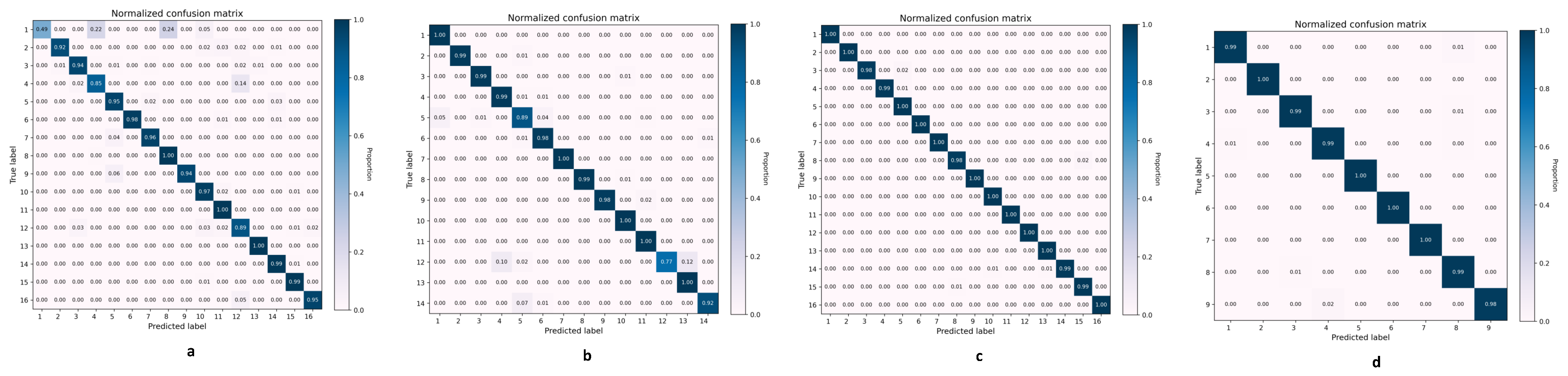
Quantitatively, S2A-Swin achieves OA improvements of 2.45%, 7.05%, 5.17%, and 0.85% on the four datasets, respectively, compared to the strongest comparison method. Furthermore, even in the case of extreme class imbalance, AA and $\kappa$ increase simultaneously, indicating that the gains are not driven by a few “large classes,” but rather broadly improve the separability of tail and easily confused classes. Taking the Pavia University dataset as an example, OA still maintains marginal advantages of approximately 0.20% and 1.07% over two strong baselines, demonstrating statistical and practical significance at the high baseline level. This is consistent with the confusion matrix. S2A-Swin’s off-diagonal terms shrink overall, and its diagonal dominance is stronger. Only in extremely difficult-to-distinguish and spatially adjacent class pairs (such as Gravel/Bricks in Pavia and Grapes Untrained/Vineyard Untrained in Salinas) are there a small amount of residual misclassification, consistent with the inherent difficulty of “nearly isospectral-adjacent” scenarios.

Overall, S2A-Swin unifies multi-scale long-range dependencies and local detail fidelity under controllable complexity through hierarchical shifting windows and spectral–spatial adaptive aggregation, resulting in a systematic, reproducible, and cross-dataset-consistent lead in the three metrics of OA, AA, and $\kappa$. Combined with our reported parameter sensitivity experiments and a unified training environment, these improvements eliminate the influence of implementation details and parameter bias, demonstrating the method’s robustness and transferability in typical HSI scenarios such as small samples, high inter-class similarity, and complex boundaries.

4.3.2. Qualitative Analysis

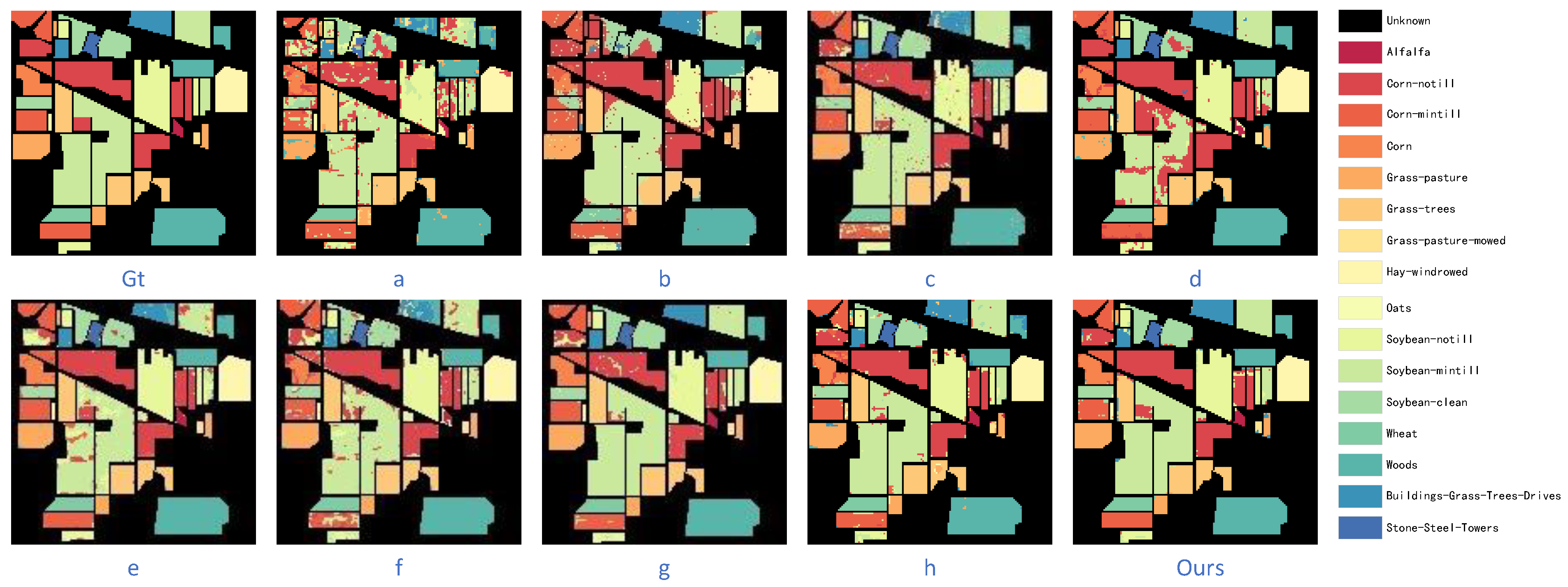
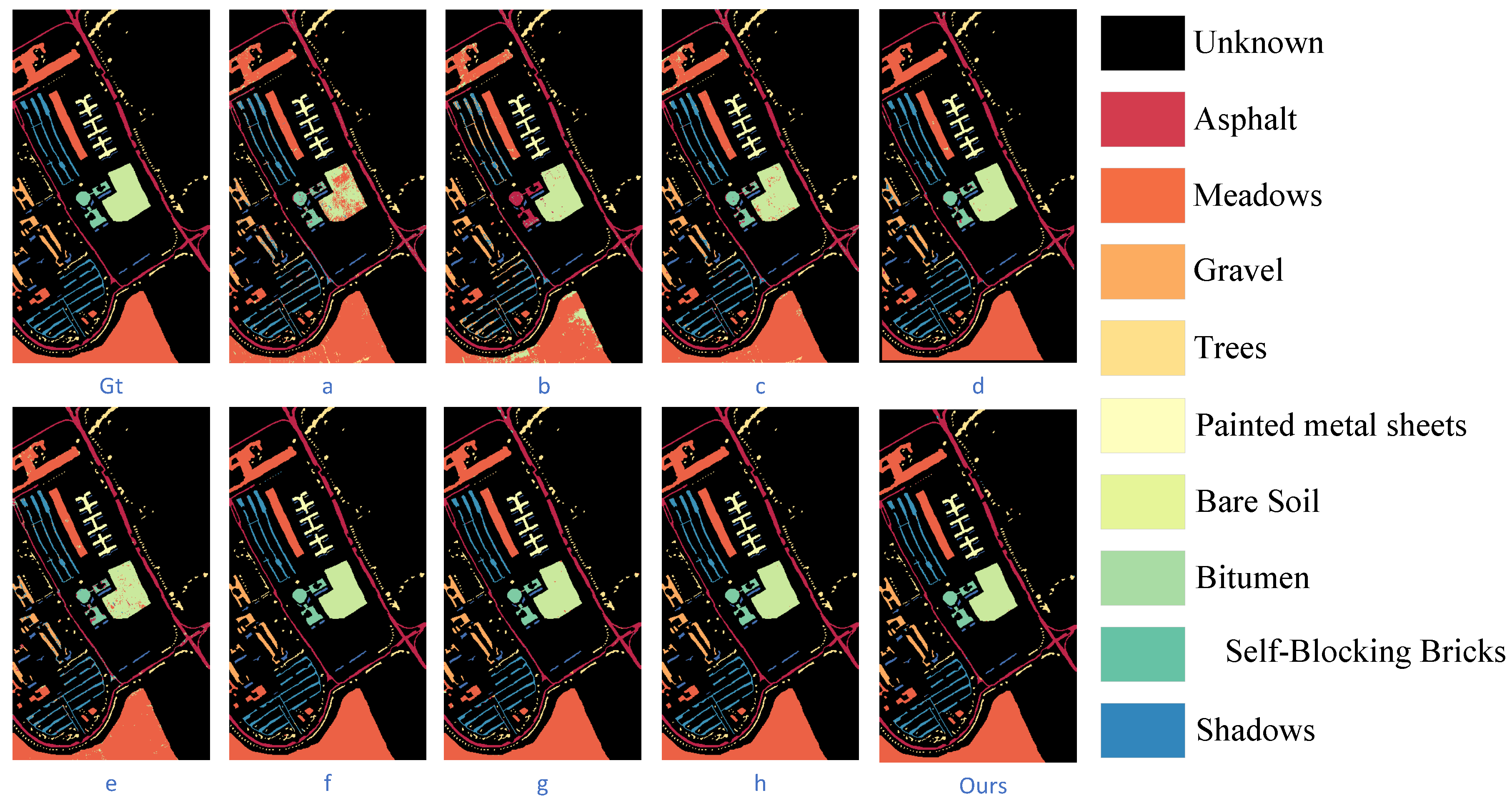
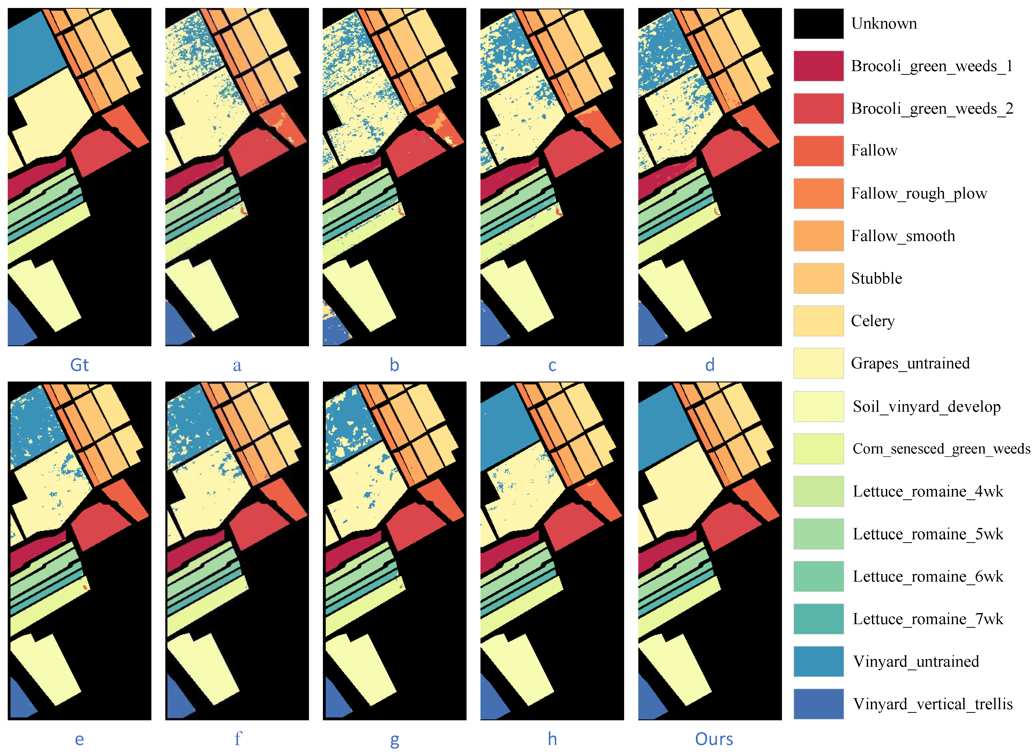
To further emphasize the superiority of our method, we also show the qualitative results and compare these with other advanced methods in Figure 7, Figure 8, Figure 9 and Figure 10. Pixel-level classifiers (1D CNN, HSIC-FM, ViT) are prone to produce significant salt-and-pepper artifacts and fragmented predictions in areas with complex textures or uncertain annotations due to the lack of spatial priors and neighborhood consistency constraints; patch-based CNN and hybrid structures (3D). Although CNN, CLOLN, and SWIN improve regional coherence through explicit spatial modeling, the local averaging effect of convolution will cause significant “boundary expansion/erosion” and topological fractures at the boundaries of high curvature or slender targets, such as “brick/commercial” and “road/runway” categories. When the spectral difference is weak and the background is similar (such as “bare soil/grass”), the decision boundary of SSFTT is unstable.

In the absence of positioning prior, VIT attention is diffuse, which brings surface smoothness but produces systematic deviations from the real geometric boundaries (such as “road”, “parking lot 2”, and “runway”). For fine-grained category combinations with highly similar appearance and spatial proximity (“soybean no-tillage/corn no-tillage”, “highway/railway/road”, “grapes untrained/vineyard”, etc.), the decision boundary of SPECTRAL-SWIN is unstable. SPECTRAL-SWIN, CLOLN, and VIT, which rely on global attention, are more likely to mistakenly incorporate irrelevant regions when representing aggregated images, diluting class-specific cues. CSIL, which primarily relies on depthwise separability and point-by-point convolution, is limited by its effective receptive field and struggles to fully capture cross-scale discriminative evidence. The fundamental reason lies in the lack of targeted structural priors for the three-dimensional spectral–spatial properties and cross-band redundancy of HSI, or the lack of fine-grained constraints on informativeness/redundancy in contextual aggregation. In contrast, S2A-Swin utilizes hierarchical and shifted window self-attention to jointly capture multi-scale long-range dependencies while preserving local details at a manageable complexity. It also selectively enhances informative bands and key neighborhoods through spectral–spatial adaptive aggregation, suppressing redundancy and interference. Combined with the multi-view consistent encoding provided by HybridSwinBlock, it mechanistically mitigates three persistent issues: pixel noise, over-smoothing boundaries, and fine-grained similarity confusion. Its visual benefits manifest in sharper edges, improved continuity of slender structures, and significantly reduced class leakage in textured areas across a wide range of scenarios. The confusion matrix in Figure 11 is highly consistent with the above phenomenon: the off-diagonal elements of the four datasets are generally sparse and nearly diagonal, with only a few misclassifications remaining in the recognized “near-isospectral–spatial proximity” difficulty points, such as Pavia’s Gravel/Bricks and Salinas’ Grapes Untrained/Vineyard Untrained. These residual confusions are more likely a reflection of intrinsic class inseparability rather than model mismatch.

Overall, S2A-Swin demonstrates systematic and interpretable advantages in the three key dimensions of “noise suppression, boundary preservation, and separation of similar classes,” resulting in higher consistency and stability between its classification maps and the ground truth across the four datasets, and demonstrating good small-sample adaptability.

4.3.3. Computational Complexity Analysis

To illustrate the computational complexity of the proposed S2A-Swin compared to other methods, we report floating-point operations (FLOPs), parameter count (Params), and inference runtime in

Table 13. FLOPs, parameters, and inference time of comparative methods on four datasets.

Methods	Indian Pines			Pavia University			BOS			Salinas Scene
	FLOPs (M)	Params (k)	Time (s)	FLOPs (M)	Params (k)	Time (s)	FLOPs (M)	Params (k)	Time (s)	FLOPs (M)	Params (k)	Time (s)
1D CNN	0.19	28.05	0.05	0.10	14.73	0.14	0.14	20.75	0.05	0.17	28.56	0.39
3D CNN	6.80	86.96	0.07	3.40	58.12	0.29	2.28	70.70	0.09	6.89	88.11	0.41
CSIL	61.56	151.44	0.73	30.78	150.54	1.63	21.51	151.31	0.66	60.94	151.44	0.92
HSIC-FM	122.47	403.58	1.52	123.64	402.68	5.90	120	403.46	1.90	119.36	403.58	7.51
ViT	3.16	333.31	0.88	1.11	155.50	2.03	1.86	216.88	0.71	3.28	343.06	3.57
SWIN	251.80	51,227.42	3.32	125.90	43,451.71	13.82	130.74	46,128.69	4.20	170.90	51,652.06	20.43
CLOLN	19.08	931.85	0.91	9.54	484.42	0.84	6.70	673.74	0.62	19.06	950.28	1.04
S2A-Swin	3.52	428.66	2.69	2.00	382.13	5.90	2.00	382.13	1.57	2.22	421.88	9.95

. Following, we define an efficiency metric $\eta$ that balances the gains in overall accuracy (OA) against the additional FLOPs and extra parameters required:

$$\eta ={\displaystyle \frac{Norm(\Delta \mathrm{FLOPs})+Norm(\Delta \mathrm{Params})+1}{\Delta \mathrm{OA}+1}},$$

where OA is expressed in percent (so $\Delta \mathrm{OA}$ is the change in percentage points) and $Norm(·)$ denotes normalization of the respective quantity. Adding 1 to both the numerator and denominator ensures positivity and avoids division by zero. A smaller $\eta$ indicates higher efficiency ( fewer additional FLOPs and parameters required to increase OA by 1%). As shown in Table 13, among the Transformer-based methods (ViT, SWIN, CSIL, CLOLN, and ours), S2A-Swin requires relatively fewer FLOPs and parameters.

5. Discussion

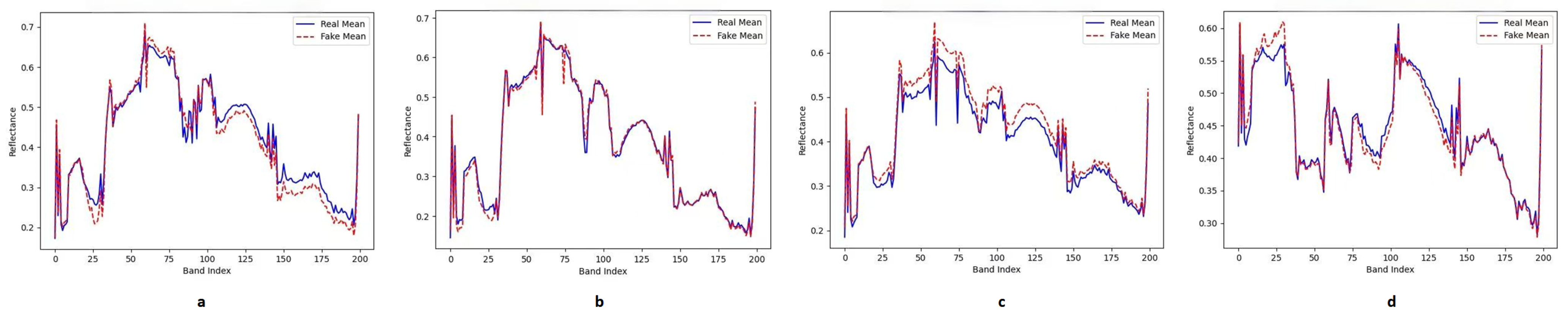
Under the extremely low supervision quota of only 10% labeled samples per class, the generalization of the classifier is mainly dominated by two types of risks: first, the prior bias of the long-tail class is amplified, and the discrimination boundary of the minority class is eroded by the majority class in the process of empirical risk minimization; second, the statistical sufficiency of the spectral–spatial three-dimensional structure is insufficient, making it difficult for the model to simultaneously learn the stable coupling of long-range dependencies and local geometry. Around these two points, the contribution of the data-side and model-side innovations of this method in the 10% scenario will be significantly “amplified”: after removing SS-cGAN, the decrease in macro-average indicators (AA, macro-F1, G-mean) and $\kappa$ will be significantly greater than that of OA, accompanied by a significant increase in the intra-class recall variance, an expansion of the off-diagonal terms of the confusion matrix in the long tail and similar classes (such as Gravel/Bricks, Grapes Untrained/Vineyard Untrained), and an earlier overfitting and lower peak in the learning curve, indicating that the benefit of SS-cGAN does not come from “data accumulation”, but from the correct shaping of the minority class distribution and spectral-space continuity. If only spectral smoothing is removed, the unphysical spectral noise corrupts the discriminative absorption features, causing the intermixing rate of near-spectral similar classes to increase most significantly. This further confirms that SSC preserves the subtle discriminative features against generative noise, causing the intermixing rate of near-spectral similar classes to increase most significantly. To intuitively illustrate this preservation and confirm that the SSC does not inadvertently cause negative “over-smoothing”, we visualize the spectral signatures in Figure 12. Using four extreme minority classes from the Indian Pines dataset as examples, it can be observed that the generated spectra (dashed red lines) tightly follow the real data’s macroscopic envelopes (solid blue lines). Most importantly, highly discriminative local features—such as the sharp absorption valleys and distinct peaks—are perfectly retained rather than being artificially flattened. This visual evidence confirms that our calibrated SSC functions as a targeted physical constraint, eliminating unnatural high-frequency GAN jitter while strictly respecting the intrinsic spectral signatures of individual classes. Meanwhile removing only spatial smoothing will manifest as a deterioration of block consistency in the classification graph and an increase in noise points, which is consistent with the key role of spatial prior in combating noise in the 10% scenario. Replacing SS-cGAN with vanilla cGAN is equivalent, even with matching generation scale, it is difficult to replicate the same improvement in AA/$\kappa$, indicating that “conditional generation with spectral-space consistency”, rather than “unconstrained amplification”, is the source of performance.

On the model side, removing the spectral window and retaining only the spatial window directly weakens cross-band alignment and near-spectral discrimination, with AA and $\kappa$ being the primary impactin

Table 14. Ablation of proposed components with 10% training samples per class on the IP dataset.

Idx	Modules				Indian Pines
	SS-cGAN	SpecWin	CrossOrder	S2A	OA (%)	AA (%)	$\mathbf{\kappa }\times \mathbf{100}$
1	✓	✓	✓	✓	96.98 ± 0.36	95.99 ± 0.47	96.56 ± 0.41
2	×	✓	✓	✓	95.21 ± 0.54	94.21 ± 0.62	94.78 ± 0.58
3	✓	×	✓	✓	95.72 ± 0.49	94.53 ± 0.58	95.11 ± 0.52
4	✓	✓	×	✓	95.86 ± 0.51	94.69 ± 0.57	95.29 ± 0.55
5	✓	✓	✓	×	95.43 ± 0.55	94.12 ± 0.63	94.91 ± 0.59
6	×	×	✓	✓	94.37 ± 0.67	93.01 ± 0.71	93.92 ± 0.69
7	×	✓	✓	×	94.72 ± 0.62	93.24 ± 0.68	94.15 ± 0.64
8	×	×	×	×	93.58 ± 0.79	92.17 ± 0.83	93.11 ± 0.81

. Disrupting or removing the execution order of cross-order attention disrupts the prior “spectral → space/space → spectral” pairings, leading to boundary erosion and breakage of slender structures in the ROI, while also releasing errors for adjacent categories in the confusion matrix. Replacing the domain perception module with a standard Swin or 2D-CNN block further amplifies these distortions under equal parameter and computational conditions, suggesting that the inductive bias of “two-dimensional windowing + order alternation” is necessary, not redundant, for the three-dimensional properties of HSI.

More importantly, under the 10% annotation quota, the two aforementioned improvement paths exhibit a synergistic effect: SS-cGAN improves the coverage and balance of the “learnable distribution” at the data level, mitigating long tails and noise, while the domain-aware hybrid Swin provides a spectral–spatial decoupling and recoupling mechanism that matches this distribution at the model level, ensuring that generated and real samples are aligned in the representation space and can be consistently utilized. The combined effect of these two approaches is evident in simultaneous improvements in AA, macro-F1, and $\kappa$, significant reductions in per-class recall variance and ECE, and a gentler rise in the learning curve with later early stopping points. This chain of evidence is particularly critical under the 10% annotation quota, as it transforms “superficial OA gains” into substantial improvements in “class balance, calibration, and robustness,” thereby avoiding misinterpretation of these improvements as incidental gains from parameter tuning or data augmentation.

6. Conclusions

In this paper, we propose a novel Transformer-based model for HSI classification, named S2A-Swin, which combines the properties of HSI with the Swin Transformer network architecture. Specifically, S2A-Swin models local and hierarchical spatial-spectral relationships while building discriminative representations for better classification. S2A-Swin primarily consists of SSC-cGAN and the HybridSwinBlock. Instead of directly applying GAN to generate dependencies, SSC-cGAN leverages spectral physical properties as constraints to reorganize image patches into overlapping cubes. At the data level, a conditional generative adversarial network (SSC-cGAN) with spectral and spatial smoothing regularization is introduced to synthesize patches of scarce categories while maintaining spectral continuity and local geometric consistency, mitigating long-tail bias and insufficient training data at the source. At the model level, a domain-aware hybrid Transformer module is constructed. Through local windowing and cross-order attention in both spatial and spectral dimensions, cross-dimensional information interaction is explicitly guided, enabling the aggregation of long-range dependencies while preserving detail fidelity with manageable complexity. HybridSwinBlock extracts hierarchical spatial–spectral relationships from these tag embeddings with the help of spatial-MSA and spectral-MSA, integrating features from the Swin Transformer module to improve discriminative ability and facilitate training. The two models form a synergistic mechanism: SSC-cGAN provides a more balanced and physically consistent “learnable distribution,” while hybrid Swin uses a matching two-dimensional window and sequential prior to achieve efficient spectral–spatial joint modeling. Experiments on four HSI datasets from different scenarios demonstrate that the proposed S2A-Swin achieves comparable results to existing state-of-the-art HSI classifiers in terms of classification accuracy and computational cost.

References

1. Willett, R.M.; Duarte, M.F.; Davenport, M.A.; Baraniuk, R.G. Sparsity and structure in hyperspectral imaging: Sensing, reconstruction, and target detection. IEEE Signal Process. Mag. 2013, 31, 116–126. [Google Scholar] [CrossRef] [Scilit]
2. Bandos, T.V.; Bruzzone, L.; Camps-Valls, G. Classification of hyperspectral images with regularized linear discriminant analysis. IEEE Trans. Geosci. Remote Sens. 2009, 47, 862–873. [Google Scholar] [CrossRef] [Scilit]
3. Chang, C.I. Hyperspectral Imaging: Techniques for Spectral Detection and Classification; Springer Science & Business Media: Berlin/Heidelberg, Germany, 2003; Volume 1. [Google Scholar]
4. Datta, D.; Mallick, P.K.; Bhoi, A.K.; Ijaz, M.F.; Shafi, J.; Choi, J. Hyperspectral image classification: Potentials, challenges, and future directions. Comput. Intell. Neurosci. 2022, 2022, 3854635. [Google Scholar] [CrossRef] [Scilit]
5. Siche, R.; Vejarano, R.; Aredo, V.; Velasquez, L.; Saldana, E.; Quevedo, R. Evaluation of food quality and safety with hyperspectral imaging (HSI). Food Eng. Rev. 2016, 8, 306–322. [Google Scholar] [CrossRef] [Scilit]
6. Santos, C.F.G.D.; Papa, J.P. Avoiding overfitting: A survey on regularization methods for convolutional neural networks. ACM Comput. Surv. (Csur) 2022, 54, 1–25. [Google Scholar] [CrossRef] [Scilit]
7. Vali, A.; Comai, S.; Matteucci, M. Deep learning for land use and land cover classification based on hyperspectral and multispectral earth observation data: A review. Remote Sens. 2020, 12, 2495. [Google Scholar] [CrossRef] [Scilit]
8. Hasan, H.; Shafri, H.Z.; Habshi, M. A comparison between support vector machine (SVM) and convolutional neural network (CNN) models for hyperspectral image classification. In IOP Conference Series: Earth and Environmental Science; IOP Publishing: Bristol, UK, 2019; Volume 357, p. 012035. [Google Scholar]
9. Song, W.; Li, S.; Kang, X.; Huang, K. Hyperspectral image classification based on KNN sparse representation. In Proceedings of the 2016 IEEE International Geoscience and Remote Sensing Symposium (IGARSS); IEEE: New York, NY, USA, 2016; pp. 2411–2414. [Google Scholar]
10. Ahmad, M. Deep Learning for Hyperspectral Image Classification. Doctoral Thesis, Università degli Studi di Messina, Messina, Italy, 2021. Doctoral Programme in Cyber Physical Systems. Available online: https://hdl.handle.net/20.500.14242/126198 (accessed on 17 March 2025).
11. Ahmed, S.F.; Alam, M.S.B.; Hassan, M.; Rozbu, M.R.; Ishtiak, T.; Rafa, N.; Mofijur, M.; Shawkat Ali, A.; Gandomi, A.H. Deep learning modelling techniques: Current progress, applications, advantages, and challenges. Artif. Intell. Rev. 2023, 56, 13521–13617. [Google Scholar] [CrossRef] [Scilit]
12. Song, H.; Kim, M.; Park, D.; Shin, Y.; Lee, J.G. Learning from noisy labels with deep neural networks: A survey. IEEE Trans. Neural Netw. Learn. Syst. 2022, 34, 8135–8153. [Google Scholar] [CrossRef] [Scilit]
13. Ullah, F.; Ullah, I.; Khan, K.; Khan, S.; Amin, F. Advances in deep neural network-based hyperspectral image classification and feature learning with limited samples: A survey. Appl. Intell. 2025, 55, 370. [Google Scholar] [CrossRef] [Scilit]
14. Islam, M.T.; Islam, M.R.; Uddin, M.P.; Ulhaq, A. A deep learning-based hyperspectral object classification approach via imbalanced training samples handling. Remote Sens. 2023, 15, 3532. [Google Scholar] [CrossRef] [Scilit]
15. Zhang, F.; Bai, J.; Zhang, J.; Xiao, Z.; Pei, C. An optimized training method for GAN-based hyperspectral image classification. IEEE Geosci. Remote Sens. Lett. 2020, 18, 1791–1795. [Google Scholar] [CrossRef] [Scilit]
16. Zhan, Y.; Hu, D.; Wang, Y.; Yu, X. Semisupervised hyperspectral image classification based on generative adversarial networks. IEEE Geosci. Remote Sens. Lett. 2017, 15, 212–216. [Google Scholar] [CrossRef] [Scilit]
17. Sun, C.; Zhang, X.; Meng, H.; Cao, X.; Zhang, J.; Jiao, L. Dual-Branch Spectral–Spatial Adversarial Representation Learning for Hyperspectral Image Classification with Few Labeled Samples. IEEE J. Sel. Top. Appl. Earth Obs. Remote Sens. 2023, 16, 1–15. [Google Scholar] [CrossRef] [Scilit]
18. Tomar, S.; Gupta, A. A review on mode collapse reducing gans with gan’s algorithm and theory. In GANs for Data Augmentation in Healthcare; Springer: Cham, Switzerland, 2023; pp. 21–40. [Google Scholar]
19. Gulrajani, I.; Ahmed, F.; Arjovsky, M.; Dumoulin, V.; Courville, A.C. Improved training of wasserstein gans. Adv. Neural Inf. Process. Syst. 2017, 30, 5769–5779. [Google Scholar]
20. Zhan, Y.; Wang, Y.; Yu, X. Semisupervised hyperspectral image classification based on generative adversarial networks and spectral angle distance. Sci. Rep. 2023, 13, 22019. [Google Scholar] [CrossRef] [Scilit]
21. Paoletti, M.E.; Haut, J.M.; Plaza, J.; Plaza, A. Deep & dense convolutional neural network for hyperspectral image classification. Remote Sens. 2018, 10, 1454. [Google Scholar]
22. Fu, W.; Lu, T.; Li, S. Context-aware compressed sensing of hyperspectral image. IEEE Trans. Geosci. Remote Sens. 2019, 58, 268–280. [Google Scholar] [CrossRef] [Scilit]
23. He, J.; Zhao, L.; Yang, H.; Zhang, M.; Li, W. HSI-BERT: Hyperspectral image classification using the bidirectional encoder representation from transformers. IEEE Trans. Geosci. Remote Sens. 2019, 58, 165–178. [Google Scholar] [CrossRef] [Scilit]
24. Yang, J.; Wu, C.; Du, B.; Zhang, L. Enhanced multiscale feature fusion network for HSI classification. IEEE Trans. Geosci. Remote Sens. 2021, 59, 10328–10347. [Google Scholar] [CrossRef] [Scilit]
25. Kong, W.; Liu, B.; Bi, X.; Pei, J.; Chen, Z. Instructional Mask Autoencoder: A Scalable Learner for Hyperspectral Image Classification. IEEE J. Sel. Top. Appl. Earth Obs. Remote Sens. 2024, 17, 1348–1362. [Google Scholar] [CrossRef] [Scilit]
26. Yang, H.; Yu, H.; Zheng, K.; Hu, J.; Tao, T.; Zhang, Q. Hyperspectral image classification based on interactive transformer and CNN with multilevel feature fusion network. IEEE Geosci. Remote Sens. Lett. 2023, 20, 5507905. [Google Scholar] [CrossRef] [Scilit]
27. Kong, W.; Liu, B.; Bi, X.; Yu, C.; Li, X.; Chen, Y. HyperSL: A Spectral Foundation Model for Hyperspectral Image Interpretation. IEEE Trans. Geosci. Remote Sens. 2025, 63, 5513119. [Google Scholar] [CrossRef] [Scilit]
28. Liu, B.; Liu, Y.; Zhang, W.; Tian, Y.; Kong, W. Spectral swin transformer network for hyperspectral image classification. Remote Sens. 2023, 15, 3721. [Google Scholar] [CrossRef] [Scilit]
29. Tang, J.; Ma, N.; Jia, C.; Tian, R.; Guo, Y. HyperEAST: An Enhanced Attention-Based Spectral-Spatial Transformer with Self-Supervised Pretraining for Hyperspectral Image Classification. IEEE J. Sel. Top. Appl. Earth Obs. Remote Sens. 2025, 18, 22241–22255. [Google Scholar] [CrossRef] [Scilit]
30. Hayes, J.; Melis, L.; Danezis, G.; De Cristofaro, E. Logan: Membership inference attacks against generative models. arXiv 2017, arXiv:1705.07663. [Google Scholar] [CrossRef] [Scilit]
31. Shokri, R.; Stronati, M.; Song, C.; Shmatikov, V. Membership inference attacks against machine learning models. In Proceedings of the 2017 IEEE Symposium on Security and Privacy (SP); IEEE: New York, NY, USA, 2017; pp. 3–18. [Google Scholar]
32. Liang, H.; Bao, W.; Shen, X. Adaptive weighting feature fusion approach based on generative adversarial network for hyperspectral image classification. Remote Sens. 2021, 13, 198. [Google Scholar] [CrossRef] [Scilit]
33. Sun, C.; Zhang, X.; Meng, H.; Cao, X.; Zhang, J. AC-WGAN-GP: Generating Labeled Samples for Improving Hyperspectral Image Classification with Small-Samples. Remote Sens. 2022, 14, 4910. [Google Scholar] [CrossRef] [Scilit]
34. Zhang, M.; Wang, Z.; Wang, X.; Gong, M.; Wu, Y.; Li, H. Features kept generative adversarial network data augmentation strategy for hyperspectral image classification. Pattern Recognit. 2023, 142, 109701. [Google Scholar] [CrossRef] [Scilit]
35. Ullah, F.; Ullah, I.; Khan, K.; Khan, S.; Wang, Q.; Algamdi, S.A.; Aldossary, H. Squeeze-SwinFormer: Spectral Squeeze and Excitation Swin Transformer Network for Hyperspectral Image Classification. IEEE J. Sel. Top. Appl. Earth Obs. Remote Sens. 2025, 18, 21400–21418. [Google Scholar] [CrossRef] [Scilit]
36. Liu, B.; Zhang, H.; Zhu, J.; Chen, Y.; Pan, Y.; Gong, X.; Yan, J.; Zhang, H. Pixel-level recognition of trace mycotoxins in red ginseng based on hyperspectral imaging combined with 1DCNN-residual-BiLSTM-attention model. Sensors 2024, 24, 3457. [Google Scholar] [CrossRef] [Scilit]
37. Lv, H.; Sun, Y.; Zhang, H.; Li, M. Hybrid 2D–3D convolution and pre-activated residual networks for hyperspectral image classification. Signal Image Video Process. 2024, 18, 3815–3827. [Google Scholar] [CrossRef] [Scilit]
38. Yao, T.; Pan, Y.; Li, Y.; Ngo, C.W.; Mei, T. Wave-vit: Unifying wavelet and transformers for visual representation learning. In European Conference on Computer Vision; Springer: Berlin/Heidelberg, Germany, 2022; pp. 328–345. [Google Scholar]
39. Yang, J.; Du, B.; Zhang, L. Overcoming the barrier of incompleteness: A hyperspectral image classification full model. IEEE Trans. Neural Netw. Learn. Syst. 2023, 35, 14467–14481. [Google Scholar] [CrossRef] [Scilit] [PubMed]
40. Yang, J.; Du, B.; Zhang, L. From center to surrounding: An interactive learning framework for hyperspectral image classification. ISPRS J. Photogramm. Remote Sens. 2023, 197, 145–166. [Google Scholar] [CrossRef] [Scilit]
41. Li, C.; Rasti, B.; Tang, X.; Duan, P.; Li, J.; Peng, Y. Channel-Layer-Oriented Lightweight Spectral-Spatial Network for Hyperspectral Image Classification. IEEE Trans. Geosci. Remote Sens. 2024, 62, 5504214. [Google Scholar] [CrossRef] [Scilit]
Figure 1. Overview of our S2A-Swin. After the preprocessing module processes the input HSI, the image patch is cropped centered at a given pixel, which is fed to the SSC-cGAN to generate pseudo samples representing the local spatial–spectral relationship. These sample embeddings are then used as input to the HybridSwinBlock, followed by an MLP to predict the label of a given pixel.
Remotesensing 18 00935 g001
Figure 2. Illustration of the IP dataset. The pseudocolor image is displayed on the left, and the corresponding ground-truth land-cover map is shown on the right, where each color represents a specific land-cover category.
Remotesensing 18 00935 g002
Figure 6. Parameter sensitivity analysis of the proposed S2A-Swin on the Indian Pines, Pavia University, Salinas Scene, and Botswana datasets. The charts display the variation of overall accuracy (OA) concerning the SSC-cGAN regularization weights, (a) α s p e c and (b) α s p a t , as well as the HybridSwinBlock receptive fields, (c) w s p a t i a l and (d) w s p e c t r a l .
Remotesensing 18 00935 g006
Figure 7. Classification maps obtained by different methods for Indian Pines. (Gt—ground truth). (a) SVM; (b) 1D-CNN; (c) 3D-CNN; (d) VIT; (e) HSIC-FM; (f) SWIN; (g) CSIL; (h) CLOLN; and (Ours).
Remotesensing 18 00935 g007
Figure 8. Classification maps obtained by different methods for BOS. (Gt—ground truth). (a) SVM; (b) 1D-CNN; (c) 3D-CNN; (d) VIT; (e) HSIC-FM; (f) SWIN; (g) CSIL; (h) CLOLN; and (Ours).
Remotesensing 18 00935 g008
Figure 9. Classification maps obtained by different methods for Pavia University. (Gt—ground truth). (a) SVM; (b) 1D-CNN; (c) 3D-CNN; (d) VIT; (e) HSIC-FM; (f) SWIN; (g) CSIL; (h) CLOLN; and (Ours).
Remotesensing 18 00935 g009
Figure 10. Classification maps obtained by different methods for Pavia University. (Gt—ground truth). (a) SVM; (b) 1D-CNN; (c) 3D-CNN; (d) VIT; (e) HSIC-FM; (f) SWIN; (g) CSIL; (h) CLOLN; and (Ours).
Remotesensing 18 00935 g010
Figure 11. Confusion matrices generated by S2A-Swin over four datasets. (a) Indian Pines. (b) Pavia University. (c) BOS. (d) Salinas Scene.
Remotesensing 18 00935 g011
Figure 12. Comparison of mean spectral signatures between real samples (solid blue lines) and SS-cGAN generated samples (dashed red lines) for four extreme minority classes in the Indian Pines dataset. (a) Class 1 (Alfalfa). (b) Class 7 (Grass-pasture-mowed). (c) Class 9 (Oats). (d) Class 16 (Stone-Steel-Towers).
Remotesensing 18 00935 g012