Article

Remote-Sensing Estimation of Evapotranspiration for Multiple Land Cover Types Based on an Improved Canopy Conductance Model

1
National Engineering Research Center for Satellite Remote Sensing Applications, Aerospace Information Research Institute, Chinese Academy of Sciences, Beijing 100101, China
2
College of Resources and Environment, University of Chinese Academy of Sciences, Beijing 100049, China
3
State Key Laboratory of Remote Sensing and Digital Earth, Aerospace Information Research Institute, Chinese Academy of Sciences, Beijing 100101, China
4
China Information Security Research Institute Co., Ltd., Beijing 102209, China
*
Author to whom correspondence should be addressed.
Remote Sens. 2026, 18(3), 513; https://doi.org/10.3390/rs18030513
Submission received: 1 January 2026 / Revised: 30 January 2026 / Accepted: 3 February 2026 / Published: 5 February 2026

Highlights

What are the main findings?
  • A new remote-sensing canopy conductance model is developed by physically integrating Jarvis’ multi-factor stress functions with the K95 canopy radiation transfer mechanism, enabling PAR to regulate stomatal conductance through canopy-absorbed radiation rather than as an empirical stress factor.
  • Based on observations from 88 global flux sites during 2015–2023, a two-stage optimization strategy differentiated by land cover types is proposed to determine the optimal combination of environmental limiting functions across 12 IGBP land cover types.
What is the implication of the main finding?
  • The proposed framework resolves the long-standing inconsistency of Jarvis-type models across heterogeneous ecosystems by introducing radiative constraints into canopy conductance modeling.
  • This mechanism-based modeling strategy enhances the physiological and radiative consistency of remote-sensing ET estimation and provides a new pathway for generating large-scale ET products under diverse land cover conditions.

Abstract

Evapotranspiration (ET) links the water cycle with the energy balance and serves as a key driving process for ecosystem functioning and water resource management. Canopy conductance (Gc) plays a central role in regulating transpiration, but many models inadequately represent its regulatory mechanisms and show varying applicability across different land cover types. This study develops a remote-sensing ET estimation approach suitable for large scales and diverse land cover types and proposes an improved canopy conductance model for daily latent heat flux (LE) estimation. By integrating the canopy radiation transfer concept from the K95 model into the multiplicative Jarvis framework, an improved canopy conductance model is developed that includes limiting effects from photosynthetically active radiation (PAR), vapor pressure deficit (VPD), air temperature (T), and soil moisture (θ). Eighteen combinations of limiting functions are designed to evaluate structural performance differences. Using observations from 79 global flux sites during 2015–2023 and integrating multi-source datasets, including ERA5, MODIS, and SMAP, a two-stage parameter optimization was applied to determine the optimal limiting function combination for each land cover type. And nine sites from nine different land cover types were selected for independent spatial validation. Temporal validation within the optimization sites shows that, at the daily scale, the model achieves a Kling–Gupta efficiency (KGE) of 0.82, a correlation coefficient (R) of 0.82, and a Root Mean Square Error (RMSE) of 27.83 W/m2, demonstrating strong temporal stability. Spatial validation over independent holdout sites achieved KGE = 0.84, R = 0.84, and RMSE = 22.53 W/m2. At the 8-day scale, when evaluated over the holdout sites, the model achieves KGE = 0.87, R = 0.88, and RMSE = 18.74 W/m2. Compared with the K95 and Jarvis models, KGE increases by about 34% and 15%, while RMSE decreases by about 38% and 12%, respectively. Relative to the MOD16 and PML-V2 products, KGE increases by about 32% and 16%, while RMSE decreases by about 33% and 17%, respectively. Comprehensive comparisons show that explicitly coupling canopy structure with multiple environmental constraints within the Jarvis framework, together with structure optimization across land cover types, can markedly improve large-scale remote-sensing ET retrieval accuracy while maintaining physical consistency and physiological rationality. This provides an effective pathway and parameterization scheme for producing ET products applicable across ecosystems.

1. Introduction

Evapotranspiration (ET) is a core process linking water, energy, and carbon cycles in terrestrial ecosystems, and it plays a key role in surface energy balance, vegetation productivity, and climate feedbacks from regional to global scales [1,2]. ET reflects the transport of water from land to the atmosphere and also serves as a key variable in studies of climate change, water resource management, and the carbon cycle [3,4]. Accurately estimating the spatiotemporal patterns of ET is essential for understanding land–atmosphere exchange processes, improving agricultural irrigation management, and evaluating ecosystem functioning [5,6].
With the rapid development of remote-sensing technology and ground-based flux observation networks, ET estimation based on multi-source Earth observation data has become an important direction in land-surface process modeling. Remote-sensing observations can provide continuous global information on energy and water fluxes, offering a robust data foundation for ET estimation [7,8,9]. Current remote-sensing-based ET estimation approaches can be grouped into three major categories: (1) empirical or data-driven models, which use statistical relationships or machine-learning methods to fit empirical equations between ET and environmental variables; (2) energy-balance physical models, such as SEBAL [10] and SEBS [11], which estimate net radiation and latent heat flux using thermal infrared land-surface temperature; and (3) physically based models represented by the Penman–Monteith (PM) equation [12], which estimate ET across diverse climate zones through the joint constraints of energy balance and surface conductance. Although global ET products such as MOD16, GLEAM, and PML-V2 are now widely available, strong surface heterogeneity, inconsistent parameterizations, and simplified physiological mechanisms still lead to systematic biases across land cover types. MOD16 shows substantial underestimation in arid and semi-arid regions [13], GLEAM insufficiently captures soil-moisture responses in high-latitude frozen areas [6], and PML-V2 exhibits energy partitioning biases in irrigated croplands [14]. The root cause of these issues lies in the current models’ inability to achieve a unified representation of physical consistency and physiological rationality [15,16,17].
In Penman–Monteith-type evapotranspiration models, canopy conductance is a key parameter linking physiological processes with energy transfer [18], and its variation directly controls vegetation transpiration rates and climate-response processes [19]. Since Jarvis [20] introduced the empirical stomatal conductance model, its simple structure and easily accessible parameters have led to its wide application in ecosystem flux analysis and remote-sensing inversion [21,22]. Physiological process-based models derived from leaf gas-exchange theory, such as the Ball–Woodrow–Berry (BWB) model [23], characterize stomatal regulation by coupling with leaf photosynthesis and exhibit good physiological consistency at the leaf scale. However, difficulties in parameter acquisition and scale expansion limit their direct application in large-scale remote-sensing evapotranspiration retrieval [24]. The Jarvis model describes the effects of air temperature (T), vapor pressure deficit (VPD), photosynthetically active radiation (PAR), and soil moisture ( θ ) on stomatal conductance through empirical limiting functions, thereby reflecting environmental stress to some extent. However, long-term studies have shown that the model exhibits considerable instability across diverse climates and land cover types. First, the selection of environmental factors lacks a unified physiological basis, and the functional forms vary widely among studies, resulting in poor model transferability [25,26,27]. On the other hand, most limiting functions are based on empirical fitting and fail to maintain physiological rationality under extreme drought, high temperature, or high VPD conditions, which leads to weak adaptability [28].
In contrast, the K95 model proposed by Kelliher et al. [29] introduces an exponential light attenuation function that links radiation transfer with canopy energy balance, thereby providing a physical basis for simulating canopy transpiration. Sellers et al. [30] further integrated energy, carbon, and water flux processes, enabling a unified representation of canopy conductance and light absorption. Mu et al. [31,32] incorporated energy-balance principles into the MOD16 product and developed a global ET retrieval framework based on the PM equation. Although these models possess strong physical rationality in terms of energy balance, they often ignore the dynamic responses of stomatal conductance to environmental stress [33], which prevents them from accurately capturing vegetation’s physiological regulation. The resulting disconnect between physiological processes and energy processes has become a major bottleneck in the development of canopy conductance models [34,35,36]. Evidence from improved models such as ETMonitor and PML-V2 indicates that incorporating canopy structure, soil-moisture constraints, and radiation transfer processes can significantly enhance the stability and accuracy of ET estimation [1,9,37].
Most current studies remain limited to single ecosystems or specific regions, lacking systematic cross-type comparisons and structural optimization analyses. At the global scale, where climate gradients are pronounced, issues related to limiting function combinations, parameter sensitivity, and energy consistency in canopy conductance models remain insufficiently addressed [38,39]. An ideal canopy conductance model should meet three key criteria: (1) it should capture the integrated effects of environmental stress on conductance, including constraints from radiation, VPD, temperature, and soil moisture; (2) it should represent the physical mechanisms of canopy radiation transfer and energy partitioning; and (3) it should remain stable and transferable across diverse land cover types.
To address these issues, this study develops a remote-sensing evapotranspiration estimation method suitable for large scales and diverse land cover types, and proposes a structurally improved canopy conductance model. Building on the empirical Jarvis framework, the model incorporates the radiation transfer concept from the K95 model and accounts for four environmental constraints (PAR, VPD, T, and θ ) to form a composite structure that reflects stomatal regulation while representing energy partitioning mechanisms. By designing 18 combinations of limiting functions and integrating multi-source datasets such as ERA5, MODIS, and SMAP together with observations from multiple global flux sites for optimization and independent validation, the study applies a two-stage parameter optimization strategy to systematically evaluate structural differences and compares the results with major ET products. The findings aim to offer new insights for developing remote-sensing ET retrieval schemes that achieve physiological rationality, energy consistency, and broad cross-surface applicability.

2. Materials

2.1. Flux Tower Data

This study used daily latent heat flux (LE) observations from 88 sites within the AmeriFlux (https://ameriflux.lbl.gov/, accessed on 21 April 2025 and ICOS (https://www.icos-cp.eu/, accessed on 27 April 2025) flux networks. These sites cover 12 International Geosphere-Biosphere Programme (IGBP) land cover types. The overall temporal coverage of the site data spans 2015–2023. Each site contains at least two years of valid observations. These data were used to optimize the model and to validate the ET estimates. All flux data were obtained using eddy-covariance systems and underwent standardized quality control and reanalysis procedures [40]. These procedures include outlier removal, gap filling, turbulence filtering, and energy balance consistency checks. The resulting dataset is suitable for multi-scale process modeling and cross-regional comparison. The spatial distribution of the sites is shown in Figure 1.

2.2. Photosynthetically Active Radiation Data

The photosynthetically active radiation (PAR) data used in this study come from the NASA MCD18C2 daily product (https://www.earthdata.nasa.gov/, accessed on 11 May 2025), which has a spatiotemporal resolution of 3 h and 0.05°. This product is generated using a radiative transfer model combined with MODIS shortwave retrievals. It directly represents the photosynthetically active photon flux available to vegetation. It also quantifies the spatial heterogeneity of light absorption within the canopy. We derived daily mean PAR by averaging eight 3-hourly observations each day. This approach enables the construction of physically consistent and temporally continuous radiation-driven time series at large scales. These data provide a reliable energy foundation for computing limitation factors in the canopy conductance model and for estimating evapotranspiration.

2.3. Vegetation Parameter Data

This study uses the normalized difference vegetation index (NDVI) and leaf area index (LAI) to characterize vegetation cover and canopy structure, both of which are essential biophysical inputs for evapotranspiration models. The NDVI data are derived from the MOD09GA_006_NDVI product, which is computed from surface spectral reflectance provided by the Terra MODIS MOD09GA product. It has a temporal resolution of one day and a spatial resolution of 500 m. The dataset can be accessed through the Google Earth Engine (GEE) platform. In this study, NDVI is mainly used to estimate canopy height for low-stature vegetation types. The LAI data are obtained from the high-accuracy HiQ-LAI product (https://github.com/tiramisu18/HiQ-LAI, accessed on 21 May 2025), which has an 8-day temporal resolution. This product is generated by reprocessing the MODIS LAI C6.1 series using the STICA algorithm. By integrating pixel quality, multi-angle observations, and spatiotemporal neighborhood information, it improves temporal continuity and spatial consistency [41]. It is suitable for large-scale and long-term analyses of canopy structure.
To obtain a smooth and physically consistent vegetation time series, we first applied the Savitzky–Golay filter [42] to remove cloud contamination and short-term noise. We then used linear interpolation to generate daily continuous LAI data. This step ensures the temporal resolution required by the canopy conductance model. The final NDVI and LAI datasets accurately capture seasonal variations and differences in vegetation structure.

2.4. Soil Moisture Data

Although stomatal regulation in deep-rooted vegetation is influenced by root-zone soil moisture, most remote-sensing-based evapotranspiration models rely on surface soil moisture due to its higher observational reliability and spatial consistency. Root-zone soil moisture products from data assimilation systems are largely model-derived and may introduce additional uncertainties. Therefore, surface soil moisture was used in this study. The surface soil moisture (0–5 cm) data are obtained from the SMAP SPL4SMGP.007 product [43], which has a 3 h temporal resolution and a 9 km spatial resolution. This product integrates microwave observations with land-surface model simulations and captures variations in surface soil moisture. The daily mean is calculated from eight observations per day. The soil physical parameters are taken from the ESWRGC (2020) global soil database [44], including soil field capacity and wilting point, both provided at a spatial resolution of 10 km. These data are used to compute the soil-moisture constraint function, which regulates soil evaporation and vegetation transpiration.

2.5. Canopy Height Data

The canopy height data are derived from the ETH Global Sentinel-2 10 m Canopy Height product, which has a spatial resolution of 10 m and an annual temporal resolution. The dataset can be accessed through the Google Earth Engine platform. The dataset is generated using machine-learning methods that integrate Sentinel-2 reflectance and ICESat-2 lidar observations. It provides an accurate representation of vegetation structural characteristics across different land cover types. Canopy height is used to estimate aerodynamic conductance and is essential for accurate LE estimation. Forest canopy height is relatively high and assumed to remain constant throughout the year, and global forest canopy height datasets derived from lidar observations are used. The canopy height of shrubs, grasslands, and croplands is relatively low and typically exhibits strong seasonal and interannual variability. NDVI is used to estimate canopy height (h) for low-stature vegetation such as shrubs, grasslands, and croplands [45]:
h = h m i n _ L C T + h m a x _ L C T h m i n _ L C T N D V I m a x N D V I m i n × N D V I N D V I m i n
In the equation, h m i n _ L C T and h m a x _ L C T represent the minimum and maximum canopy heights for a specific land cover type. N D V I m i n and N D V I m a x represent the minimum and maximum NDVI. The value of h m i n _ L C T is set to 0.002 m, while h m a x _ L C T is set to 5, 2.5, 0.5, 0.5, and 0.5 m for savannas, cropland, grassland, shrubland, and barren land, respectively.

2.6. Meteorological Forcing Data

The meteorological driving variables in this study are obtained from the ERA5-Land Daily Aggregated dataset released by the European Centre for Medium-Range Weather Forecasts, with a spatial resolution of 0.1° and daily temporal resolution. This product provides key land-surface meteorological variables worldwide, including air temperature, dew-point temperature, surface pressure, wind speed, and net radiation. ERA5-Land is generated using an advanced land-surface model and a four-dimensional variational assimilation system that integrates multi-source observations within a unified physical framework, resulting in strong consistency and physical reliability across climate zones. For evapotranspiration processes, air temperature and dew-point temperature determine the vapor pressure deficit and directly influence stomatal conductance. Wind speed regulates aerodynamic resistance and affects turbulent exchange. Net radiation and air pressure together form the boundary conditions for the surface energy balance and serve as key inputs to the PM and PT equations. Owing to its stable spatiotemporal performance, ERA5-Land is particularly suitable for canopy conductance modeling across vegetation types and geographic regions.

3. Methods

3.1. Remote-Sensing Algorithms for ET

The water cycle and energy cycle are linked through ET and latent heat LE such that the latent heat of vaporization ET λ = LE. λ is the latent heat of vaporization. This study divides land-surface evapotranspiration into three components, including evaporation from the wet canopy surface ( L E i ), vegetation transpiration ( L E t ), and soil evaporation ( L E s ). Canopy conductance is the key parameter in the PM equation for estimating vegetation transpiration and is usually upscaled from leaf stomatal conductance [14]. In this study, canopy conductance is calculated from stomatal properties and then used in the PM equation to estimate vegetation transpiration. The PT model is a simplified form of the PM equation and can estimate evaporation under conditions without water stress, such as open-water evaporation and evaporation from the wet canopy surface. Combining the PT model with a soil-moisture constraint function allows the estimation of soil evaporation [46]:
L E = L E i + L E t + L E s

3.1.1. Vegetation Transpiration

When the underlying surface is vegetation, the surface conductance term in the PM equation is represented as canopy conductance. This parameter is the core of the PM equation and describes the transpiration capacity of different vegetation surfaces. The equation for calculating vegetation canopy transpiration using the PM equation is as follows:
L E t = Δ R n c + ρ a C p V P D G a Δ + 1 + G a / G c γ
In the equation, L E t is vegetation transpiration (W/m2); Δ is the slope of the saturation vapor pressure-temperature curve; ρ a is the air density (kg/m3); C p is the specific heat of air at constant pressure, set to 1013 J/(kg·K); V P D is the vapor pressure deficit (kPa); G c is the canopy conductance (m/s); and G a is the aerodynamic conductance (m/s), which is calculated from wind speed and canopy height [47].
The vapor pressure deficit can be calculated using air temperature ( T , °C) and dew-point temperature ( T d e w , °C):
e s = 0.6108 e x p 17.27 T T + 237.3
e a = 0.6108 e x p 17.27 T d e w T d e w + 237.3
V P D = e s e a
e s denotes saturated vapor pressure (kPa), and e a denotes actual vapor pressure (kPa).

3.1.2. Evaporation from the Wet Canopy Surface

When air humidity is high or after rainfall, part of the liquid water on canopy leaves undergoes direct evaporation. This saturated-water evaporation can be estimated using the simplified form of the PM equation, namely the Priestley–Taylor (PT) equation [48]:
L E i = f w e t α Δ Δ + γ R n c
R n c = R n f c
R n s = R n 1 f c
In the equation, L E i is the evaporation of canopy-intercepted water, in W/m2. R n c is the canopy net radiation, in W/m2, representing the portion of net radiation received by the canopy while ignoring canopy heat flux. Therefore, R n c represents the total available energy for evaporation from the wet canopy surface and plant transpiration. The surface net radiation can be partitioned into canopy net radiation R n c and soil net radiation R n s using the vegetation cover fraction f c . The vegetation cover fraction can be calculated from LAI [49]. Canopy heat flux was not considered in the partitioning of available energy. Due to the relatively large biomass, canopy heat flux can have a non-negligible influence on the energy balance of tall forests at sub-daily (half-hourly to hourly) time scales, particularly through daytime heat storage and nighttime heat release processes [50]. However, at the daily or longer time scales, canopy heat storage typically exhibits a pronounced diurnal compensation between positive and negative fluxes, which substantially reduces its contribution to the daily mean available energy partitioning [51].
f w e t is the fraction of the wet canopy. Mu et al. [32] modified the calculation for the condition where relative humidity (RH) is below 0.7. The calculation formula is as follows:
f w e t = 0 ,           R H < 0.7 R H 4 ,           R H 0.7
R H = e n e s

3.1.3. Soil Evaporation

Soil evaporation is simpler than vegetation transpiration, and its rate mainly depends on soil moisture content. Zhang et al. [52] represented the effect of soil moisture on soil evaporation rate using the ratio of cumulative rainfall to equivalent evaporation. Purdy et al. [48] directly used SMAP-retrieved soil moisture to compute the fraction of available soil water. García-Gutiérrez et al. [53] compared the two approaches using two PM-based models and found that the soil-moisture-based method yielded higher accuracy. Therefore, the soil evaporation calculation is expressed as follows:
L E s = f w e t + f r e w 1 f w e t α Δ Δ + γ R n s G
f r e w = θ θ w p θ f c θ w p
In the equation, f r e w represents the relative extractable water. θ is the soil moisture (m3/m3), and θ w p and θ f c represent the wilting point and field capacity, respectively. G is the soil heat flux (W/m2). It can be calculated as follows [54]:
G = R n Γ c + 1 f c Γ s Γ c
In the equation, Γ c and Γ s are empirical coefficients for fully vegetated cover and bare soil, with values of 0.05 and 0.315, respectively.

3.2. Improvement of the Canopy Conductance Model

The Jarvis model is a typical empirical multiplicative model that usually involves a series of single-factor modifiers, such as photon flux density, temperature, humidity, ambient CO2 concentration, and leaf water potential, while often ignoring the interactions among these variables:
g s = g s m f P A R f V P D f T f C s f φ
In the equation, g s is the leaf stomatal conductance (m/s), and g s m is the maximum leaf stomatal conductance (m/s). f P A R , f V P D , f T , f C s , and f φ represent the influence functions of photosynthetically active radiation (PAR, W/m2), vapor pressure deficit (VPD, kPa), air temperature (T, ℃), atmospheric CO2 concentration (ppm), and water potential (MPa) on leaf stomatal conductance. Each influence function takes values between 0 and 1. The selection and adjustment of influencing factors may vary depending on research needs.
As a key parameter linking vegetation physiological regulation with surface energy exchange, canopy conductance is primarily controlled by photosynthetically active radiation, vapor pressure deficit, air temperature, and soil moisture, which characterize its main responses to energy demand and water stress [55,56,57]. This study simulates stomatal conductance using four key environmental factors: PAR, VPD, T, and soil moisture (θ). For the upscaling approach, our analysis covers multiple land cover types; therefore, we did not adopt the simple LAI-weighted method, nor did we use formulations that separate sunlit and shaded leaves. Instead, we selected an intermediate-complexity upscaling scheme by using the big-leaf approach and incorporating canopy radiation transfer following the K95 model [29]. Based on these considerations, we developed a new canopy conductance model:
G c = g s m k Q l n P A R + Q P A R e x p k Q L A I + Q f V P D f T f θ
In the equation, G c is the canopy conductance (m/s); k Q is the shortwave radiation extinction coefficient, set to 0.6; and Q is the photosynthetically active radiation at which conductance reaches half of its maximum, set to 30 W/m2 [58].
Different environmental factors regulate stomatal conductance with markedly different response patterns and intensities, which are mainly reflected in the mathematical forms of limiting functions and their attenuation behavior under extreme conditions. Previous studies have used segmented threshold functions, exponential decay functions, or smooth inverse functions to describe the nonlinear inhibitory effects of temperature and VPD [59,60,61]. In contrast, soil moisture constraints show distinct structural differences among relative available water formulations, empirical power functions, and linear functions defined over the wilting point–saturation range [62,63]. Therefore, this study constructs a combination space using two air temperature functions, three VPD functions, and three soil moisture functions that are widely adopted in the literature and differ clearly in form (Table 1), which yields 18 representative sets of environmental limiting functions to evaluate how different structural assumptions affect canopy conductance performance across land cover types.

3.3. Model Optimization

To systematically evaluate how different limitation-function structures affect canopy conductance simulation and ET estimation, this study applied a unified optimization procedure to 18 combinations of environmental limitation functions. Model performance was assessed by comparing simulated LE with LE measurements from flux towers. We used data from 79 sites for model optimization. For each site, multi-year observations were divided chronologically into calibration and temporal validation samples at a 4:1 ratio, allowing the model to learn seasonal patterns while testing its extrapolation ability in independent periods. For each land cover type, the first 80% of the data from all sites belonging to that type are pooled together to form a unified calibration dataset for joint parameter optimization, while the remaining 20% are combined into a temporal validation dataset.
Parameter estimation was conducted using the Sequential Least Squares Programming algorithm to perform constrained optimization. The optimization objective combined Kling–Gupta efficiency (KGE) [68], correlation coefficient (R), Root Mean Square Error (RMSE), and mean absolute error (MAE). KGE was used as the primary performance metric, and the optimization updated parameters by minimizing the loss function (1 − KGE). R, RMSE, and MAE were monitored during optimization to avoid bias accumulation caused by fitting only temporal trends:
K G E = 1 R 1 2 + α 1 2 + β 1 2
α is the ratio of the standard deviation of the simulated values to that of the observed values, and β is the ratio of the mean simulated value to the mean observed value. KGE is less than 1, and a larger KGE indicates better agreement between the simulated and observed results.
The optimization procedure consists of two stages. In the first stage, only the parameters within the limitation functions are optimized, while g s m is fixed, with its value for each land cover type taken from Mu et al. [32]. This stage aims to compare the applicability of different limitation-function combinations and identify the best combinations for each land cover type without introducing extra structural degrees of freedom. In the second stage, after determining the optimal function structure for each land cover type, g s m is introduced as an optimization parameter and jointly calibrated with the corresponding limitation-function parameters to improve the magnitude matching of canopy conductance and evapotranspiration. During Stage 2, g s m was constrained within a physiologically reasonable range of 0.002–0.04 m/s [9,29,69] to avoid unrealistic solutions during optimization. This range covers typical canopy-scale conductance magnitudes reported in previous eco-physiological and evapotranspiration studies. This strategy effectively separates the contributions of function-structure differences and parameter-scale differences to model performance, ensuring that the final optimal combination is both mechanistically reasonable and quantitatively optimal.

4. Results

4.1. Performance of Different Constraint Combinations

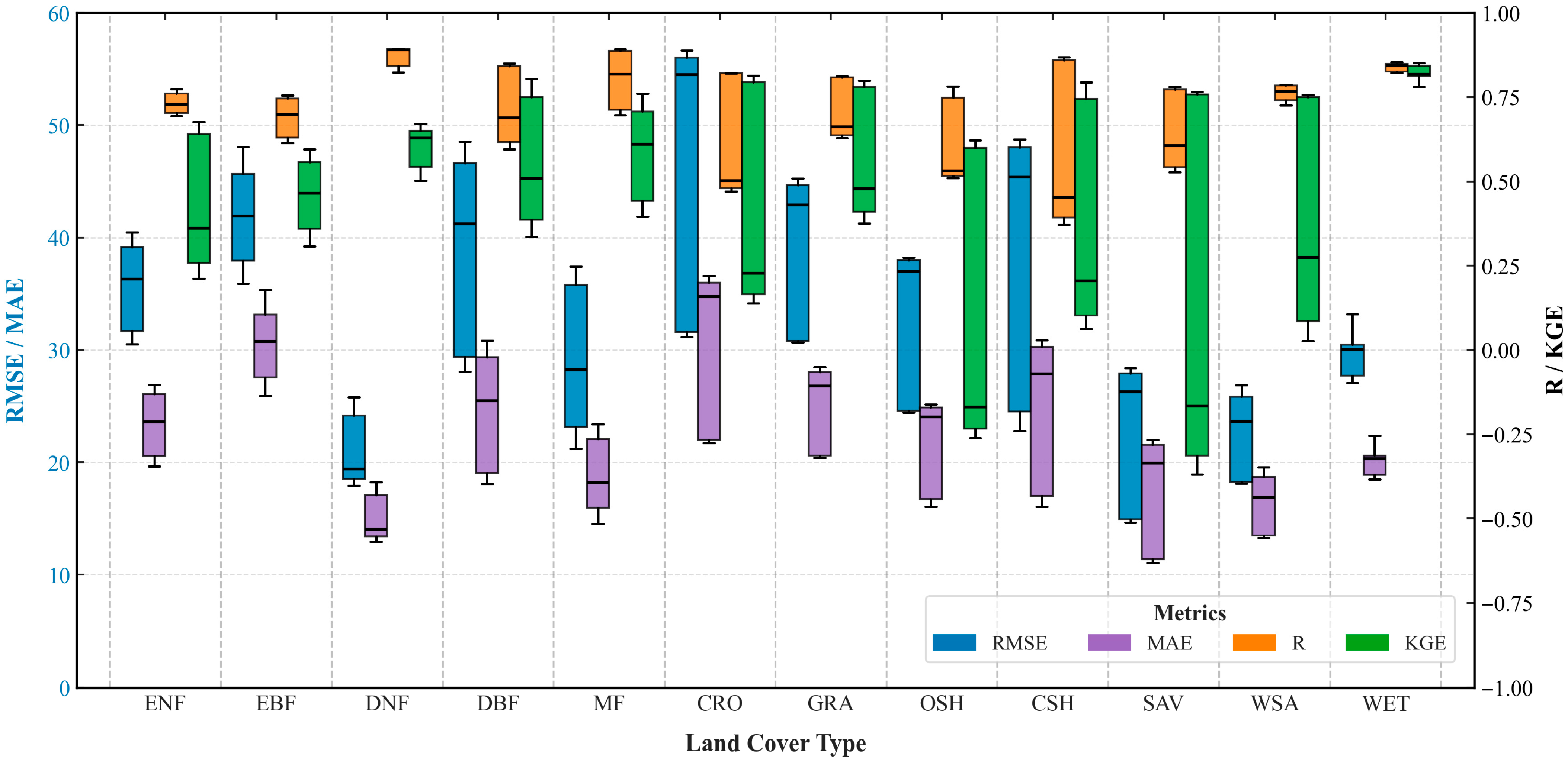
Under a fixed maximum stomatal conductance, the 18 combinations of limitation functions were optimized using a unified procedure. Figure 2 shows the overall performance distribution of different limitation-function combinations across land cover types. The performance range differs substantially among land cover types. Overall, the performance range increases along the gradient from wetlands to forests, croplands, and arid regions, indicating a stratified pattern of structural stability driven by hydrothermal conditions. Wetlands (WET) show the highest performance, with KGE values consistently between 0.78 and 0.85. Their correlation coefficients (R) generally exceed 0.8, and both RMSE and MAE remain low. This indicates that the model structure exhibits high consistency under water-abundant and energy-limited environmental conditions. Among forest land cover types, evergreen broadleaf forests (EBF) and deciduous needleleaf forests (DNF) show the most stable performance, with KGE ranges of 0.31–0.60 and 0.50–0.67, indicating that the model can reproduce ET variations well across different structural forms. Evergreen needleleaf forests (ENF), deciduous broadleaf forests (DBF), and mixed forests (MF) exhibit slightly larger KGE dispersion, with ENF showing the largest variation (0.46), suggesting high sensitivity of ENF to model structural choices. Grasslands (GRA) and croplands (CRO) show moderate performance variability caused by structural differences. Savannas (SAV) and shrublands (OSH, CSH) show the least stability, with KGE ranges in SAV exceeding 1.0 and substantial dispersion in error metrics, indicating that model performance is highly sensitive to structural forms in arid and semi-arid ecosystems.
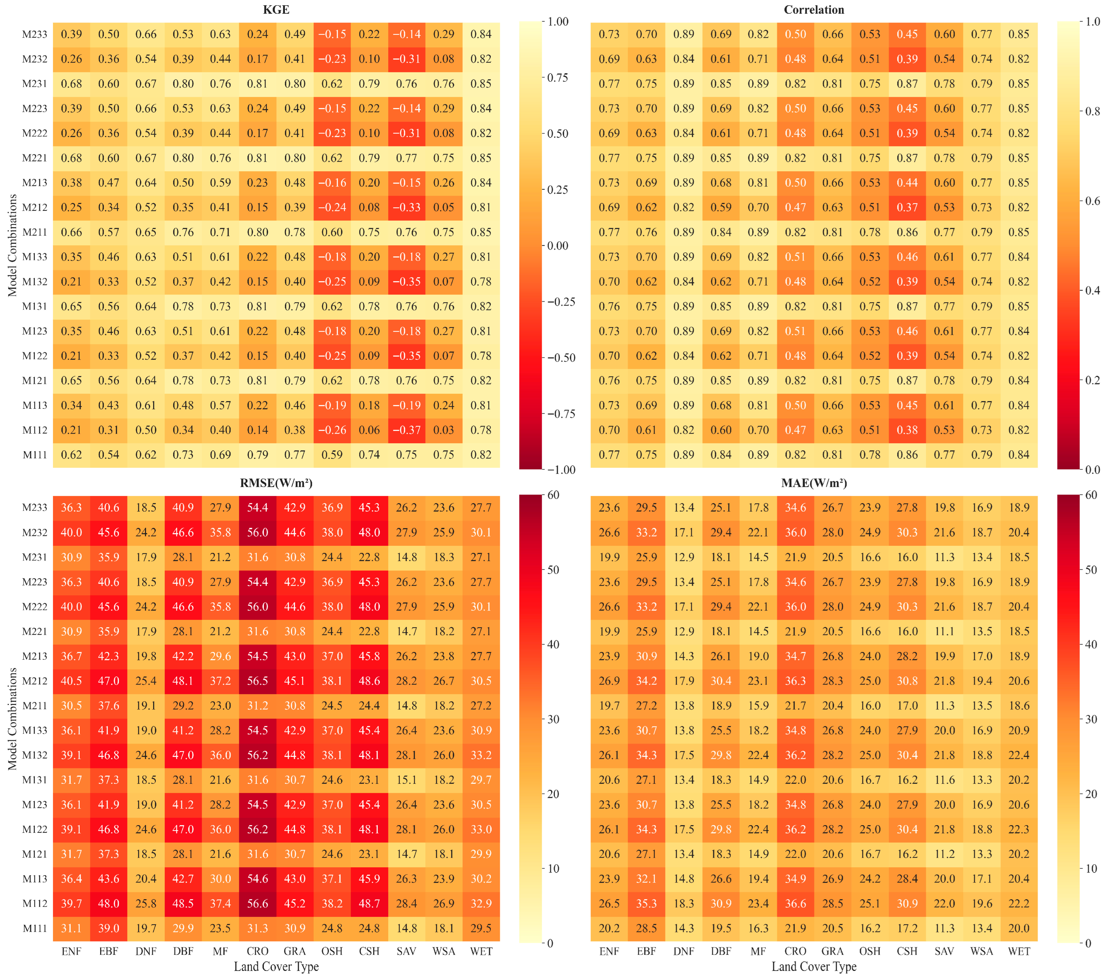
Figure 3 shows the detailed optimization results for different combinations across land cover types. The effects of the constraint factors display a clear hierarchy, with soil moisture being the most influential, followed by VPD, while temperature plays the weakest role. The three types of f θ differ substantially in performance. W1 performs best across all land cover types, with an average KGE of 0.73 and an average RMSE of 25.77 W/m2. In contrast, W2 and W3 yield much lower average KGE values of only 0.23 and 0.36, and their RMSE increases to 39.02 W/m2 and 35.55 W/m2, respectively. The difference is most pronounced in arid and semi-arid ecosystems (e.g., SAV, OSH, and CSH), where W2 and W3 often cause sharp drops in KGE, sometimes yielding negative values. In contrast, W1 maintains stable trend representation and error control. This indicates that W1 best captures soil water availability and is the most robust moisture-limitation formulation across ecosystems. Although the parameters of W1 are not directly derived from soil-type normalization, they establish a more robust data-driven constraint through the optimized parameter x. In contrast, the global soil thresholds (10 km) used by W2 and W3 are severely mismatched with the flux tower site scale, and the noise introduced by this mismatch outweighs the benefits of physical normalization. The VPD limitation functions have a weaker influence on model performance than soil moisture, but they show a consistent improvement trend. The average KGE values of V2 and V3 are very similar, around 0.5, and both are slightly higher than the 0.42 of V1. This indicates that a smoother VPD response can better represent the suppression effect on stomatal conductance. Wetlands are the only exception because their water supply is consistently abundant, making them the least sensitive to VPD formulations. The temperature limitation functions have the weakest influence. A slight advantage of T2 over T1 appears in most land cover types, with an average KGE of 0.45, slightly higher than the 0.43 of T1. Overall, the model performance depends most strongly on the soil moisture limitation function. In contrast, VPD and temperature mainly affect the smoothness of the response and its seasonal variation, but they are not strong enough to shift the dominant control processes.

4.2. Optimal Constraint Function Selection

The optimal combinations of limitation functions obtained from the second optimization are summarized in Table 2. Under the optimal structure, the model achieves high accuracy, with KGE ranging from 0.68 to 0.91 and R exceeding 0.75 for all land cover types, indicating that the unified optimization framework enables stable simulation of ET dynamics across diverse surface conditions. The best-performing types are mixed forest (MF, KGE = 0.91) and deciduous needleleaf forest (DNF, KGE = 0.87), while open shrubland (OSH, KGE = 0.68) shows the lowest performance, reflecting a clear correspondence between model structure and surface hydrothermal conditions.
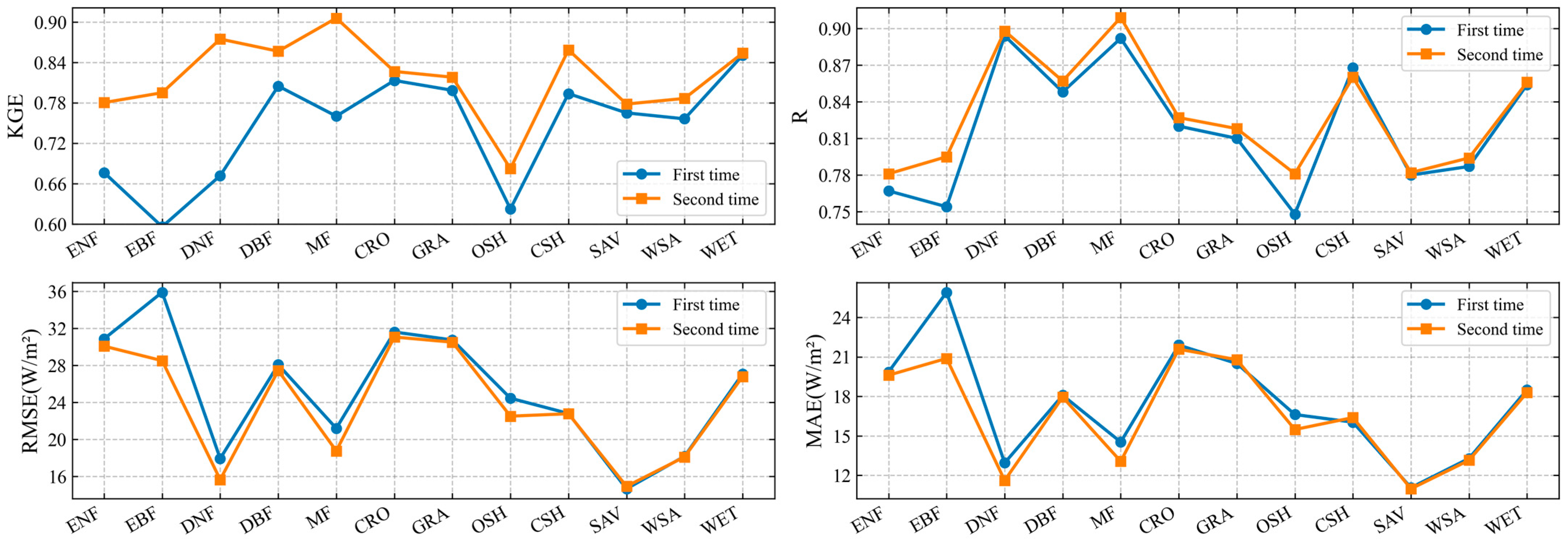
Figure 4 shows the comparison between the two optimization stages, and the model performance improves overall after the second optimization. KGE improves significantly in most land cover types, especially in forest and shrub ecosystems; for example, the EBF KGE increases by 0.40 with an RMSE reduction of 7.4 W/m2, and the KGE of CSH increases by 0.65. This indicates that under high LAI conditions, the value of gsm can substantially influence the physical representation of the evapotranspiration process. In contrast, the performance improvement in croplands and savannas is smaller, suggesting that these land cover types were already relatively stable in the first optimization.

4.3. Validation of LE Against Flux Tower Measurements

4.3.1. Validation over Optimization Sites

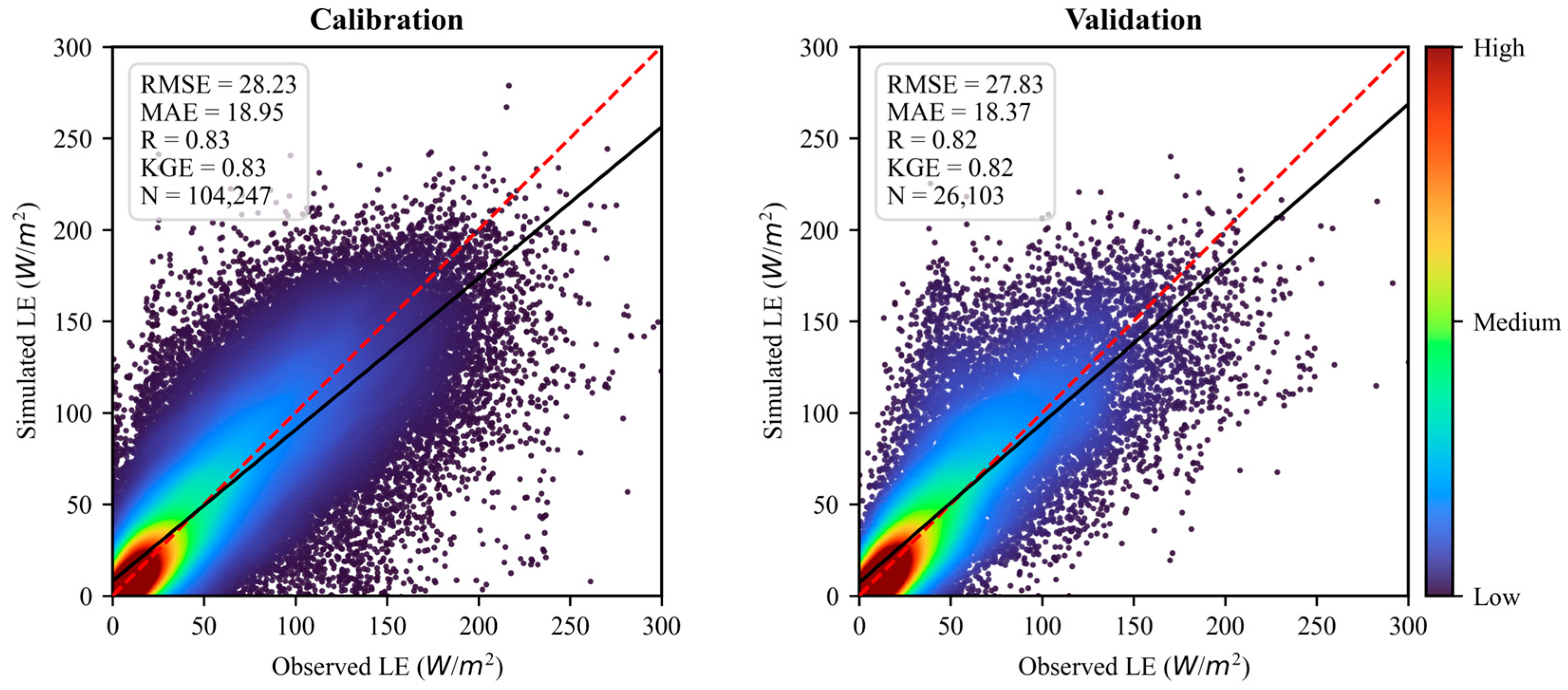
Figure 5 presents the model performance for the temporal holdout evaluation conducted within the optimization sites, where multi-year observations at each site were chronologically divided into calibration and validation subsets. Overall, the model exhibits highly consistent performance in both stages, indicating that the optimized canopy conductance parameterization remains temporally stable without overfitting within the same sites. During calibration, the model achieved a KGE of 0.83, an R of 0.83, an RMSE of 28.23 W/m2, and an MAE of 18.95 W/m2, reflecting strong consistency and low systematic error. The validation stage shows only minor changes in performance metrics, suggesting that the model parameters remain stable across time samples without noticeable drift. Most data points cluster near the 1:1 line, with good agreement between simulated and observed values in the moderate latent heat flux range. Deviations occur mainly in the high-flux region and appear in both calibration and validation, yet the overall pattern remains consistent. This suggests that the uncertainties may originate from energy-balance closure errors or observational limitations of flux towers [70].
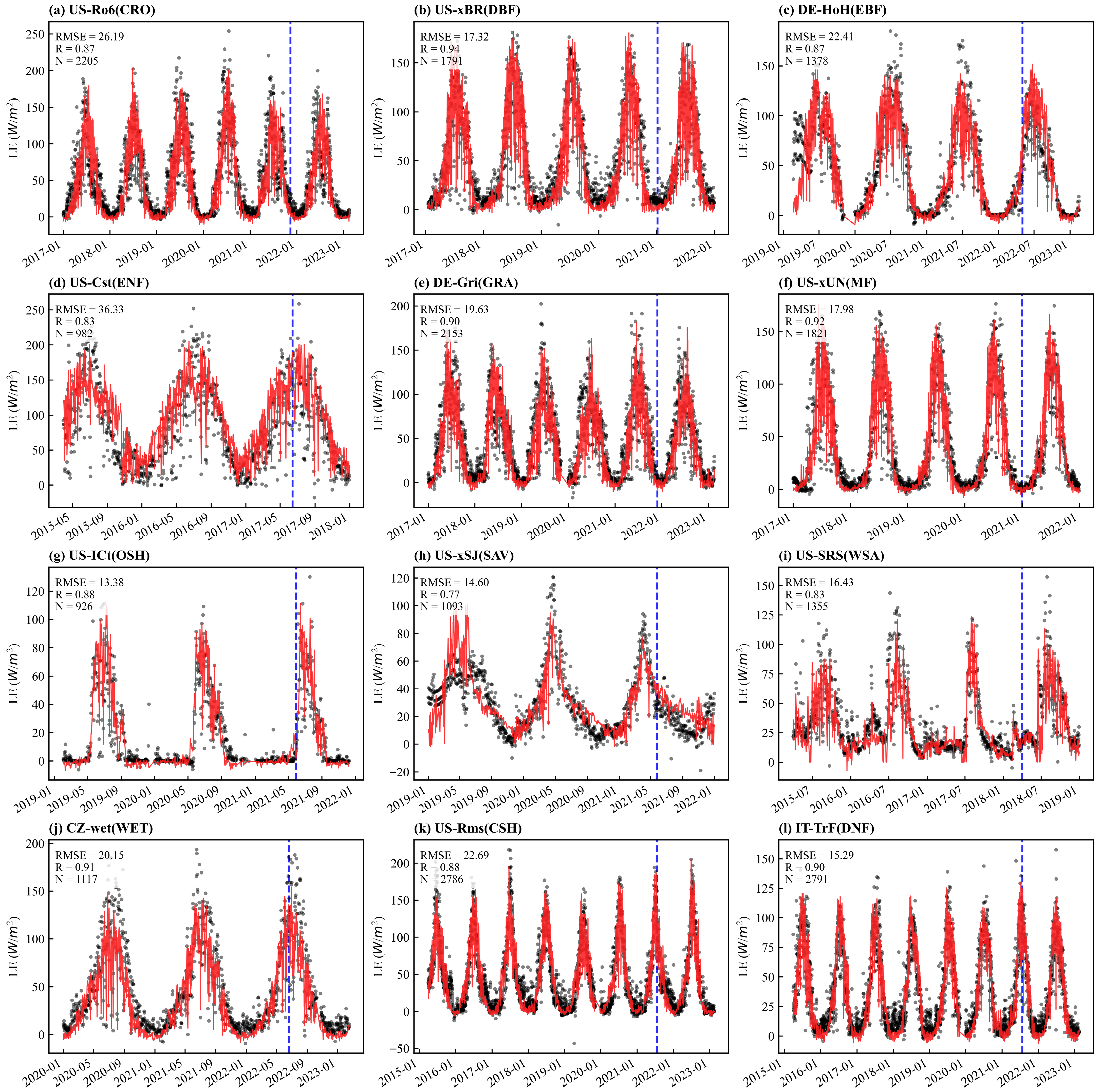
By selecting one flux site from each IGBP class to plot LE time series (Figure 6), the model generally reproduces the seasonal variability and peak timing of observed LE across different land cover types, within the same optimization sites, with no abrupt change in fitting quality before and after the calibration–validation boundary indicated by the blue dashed line. Consistency is generally higher for forest types, where the correlations reach R = 0.94 for US-xBR (DBF) and R = 0.92 for US-xUN (MF), with RMSE values of 17.32 W/m2 and 17.98 W/m2, respectively. The DNF type also maintains low errors (RMSE = 15.29 W/m2, R = 0.90), indicating strong capability in capturing temporal dynamics over land cover types with stable canopy structure and transpiration-dominated processes. By contrast, US-cST (ENF) exhibits larger errors (RMSE = 36.33 W/m2, R = 0.83), with stronger simulated amplitudes during the spring and summer seasons. For savanna and shrubland sites, LE simulations show larger summer amplitudes and more pronounced deviations under high-flux conditions, consistent with patterns observed in scatter plots, while still maintaining a reasonable representation of seasonal cycles overall.

4.3.2. Validation over Holdout Sites

To further evaluate the spatial transferability of the model, nine sites representing different land cover types were selected for LE simulation and validation, and these sites were completely excluded from the two-stage optimization process described in Section 3.3. These sites, hereafter referred to as holdout sites, were not involved in limitation-function selection, parameter estimation, or any intermediate evaluation procedure. They were used only for the independent assessment of model performance after the optimal parameterization had been finalized.
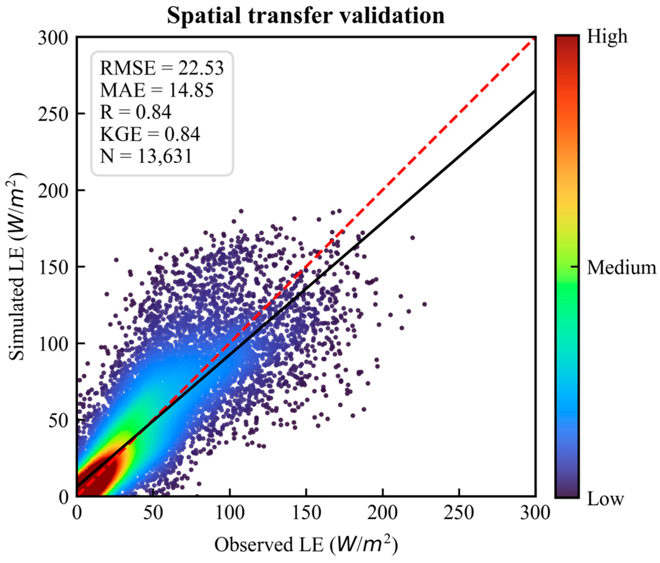
Figure 7 shows the scatter relationship between simulated and observed LE over all holdout samples. The data points cluster closely around the 1:1 line, indicating that the model retains strong agreement with observations even at sites that were never seen during optimization. Over the holdout sites, the model achieves a KGE of 0.84, an R of 0.84, an RMSE of 22.53 W/m2, and an MAE of 14.85 W/m2. Notably, the accuracy at the holdout sites is slightly higher than the overall accuracy of the optimization sites. This is closely related to the cross-site joint optimization strategy adopted for each land cover type in this study. Model parameters are optimized using the combined characteristics of multiple sites within the same land cover type, and the optimization dataset inevitably includes sites with complex climates, high observational noise, or extreme environmental stress [71,72,73]. These highly heterogeneous sites ensure parameter generality but also reduce the overall statistical performance [74,75]. In contrast, the holdout sites serve only as independent application cases for the parameterized model; therefore, it is possible that their conditions are less dominated by extremes or idiosyncratic behaviors that depress the aggregate statistics of the heterogeneous optimization pool [76].
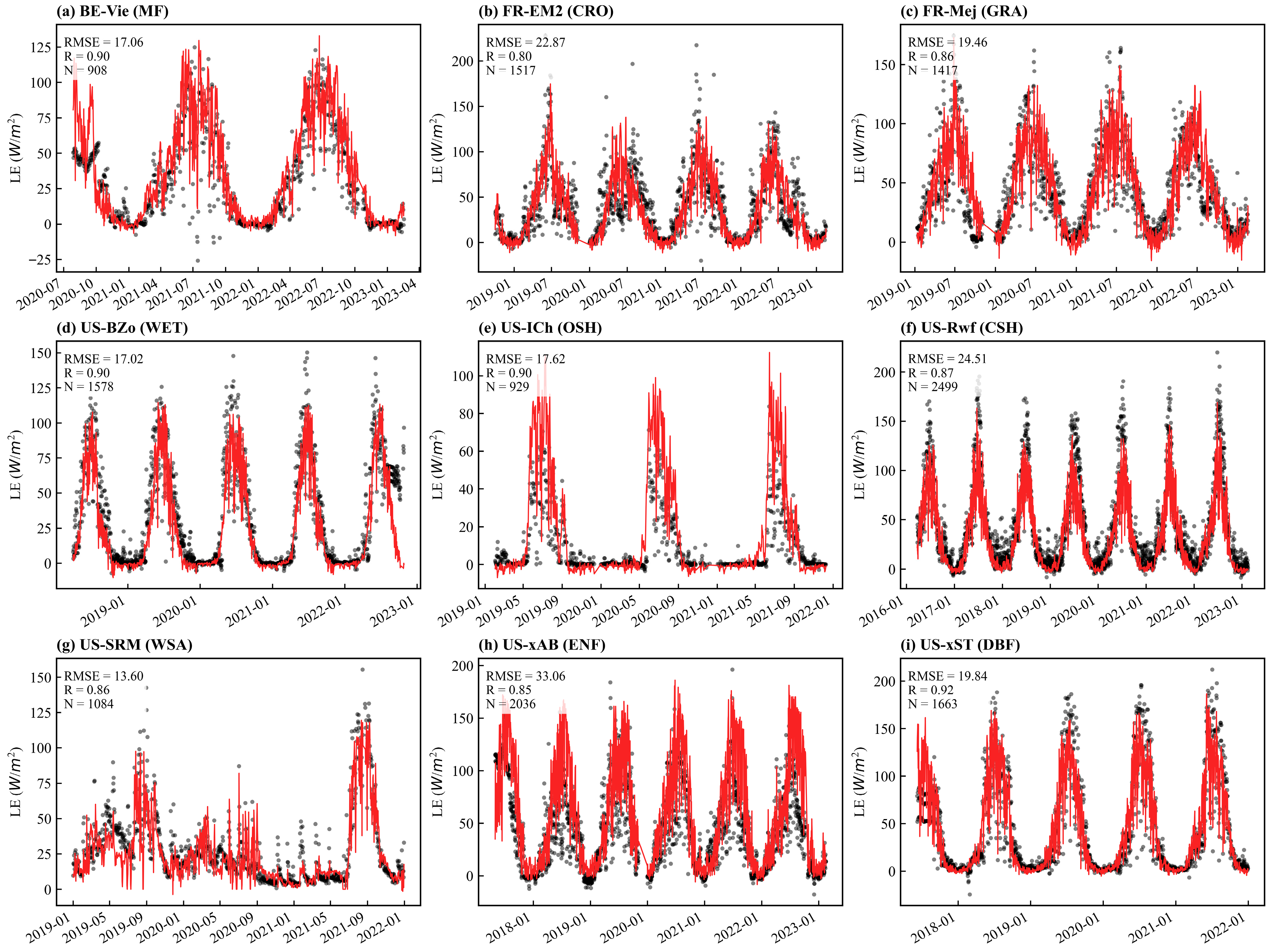
Figure 8 shows the time series from these sites. The model successfully reproduces the seasonal variability and peak timing of LE across these independent locations. Despite differences in canopy structure, climate background, and energy conditions, no systematic degradation of performance is observed. This indicates that the optimized canopy conductance formulation is not confined to the characteristics of the calibration sites, but captures more generalizable mechanisms governing vegetation transpiration and surface evaporation.

4.4. Comparison with Other ET Products

To further evaluate the applicability of the model for large-scale evapotranspiration estimation, this study selected two representative medium-to-high resolution remote-sensing ET products, MOD16 [32] and PML-V2 [77], for comparative validation. Both products use an 8-day compositing period and have a spatial resolution of 500 m. Before validation, ET (mm/day) was converted to equivalent LE (W/m2) using Equation (18), where 86,400 converts from seconds to days, λ is the latent heat of vaporization and is set to 2.45 MJ/kg [5], and ρ is the density of water (1000 kg/m3). The daily LE estimates from this study were aggregated into an 8-day composite to ensure consistency in comparison. Figure 7 presents the comparison of latent heat flux (LE) estimates at nine holdout sites:
L E = λ ρ 86400 E T
As shown in Figure 9, the RMSE of our model is 18.74 W/m2, the MAE is 12.29 W/m2, the KGE is 0.87, and R is 0.88. In comparison, MOD16A2 shows an RMSE of 27.94 W/m2 and a KGE of 0.66. PML-V2 has an RMSE of 22.51 W/m2 and a KGE of 0.75. These results show that the optimized model has the lowest error and highest correlation among the three, indicating that it captures flux variations more accurately at high temporal resolution. The scatterplots further illustrate that the model outputs align more closely with the 1:1 line, with substantially smaller deviations in the high-flux range compared with MOD16 and PML-V2. This improvement in accuracy is primarily attributed to advances in model structure and physiological constraints. Unlike the empirical ET parameterization used in MOD16, our model explicitly incorporates three stomatal limitation functions, and the optimized maximum stomatal conductance suppresses excessive ET under hot and dry conditions. The Penman–Monteith scheme in MOD16, based on the minimum-resistance assumption, tends to systematically overestimate ET under strong radiation and dry conditions [32]. Although PML-V2 uses an energy-partitioning approach for latent heat flux, its stomatal conductance parameterization still relies on a simplified Jarvis formulation, which often leads to insufficient ET response during seasonal transitions [77].
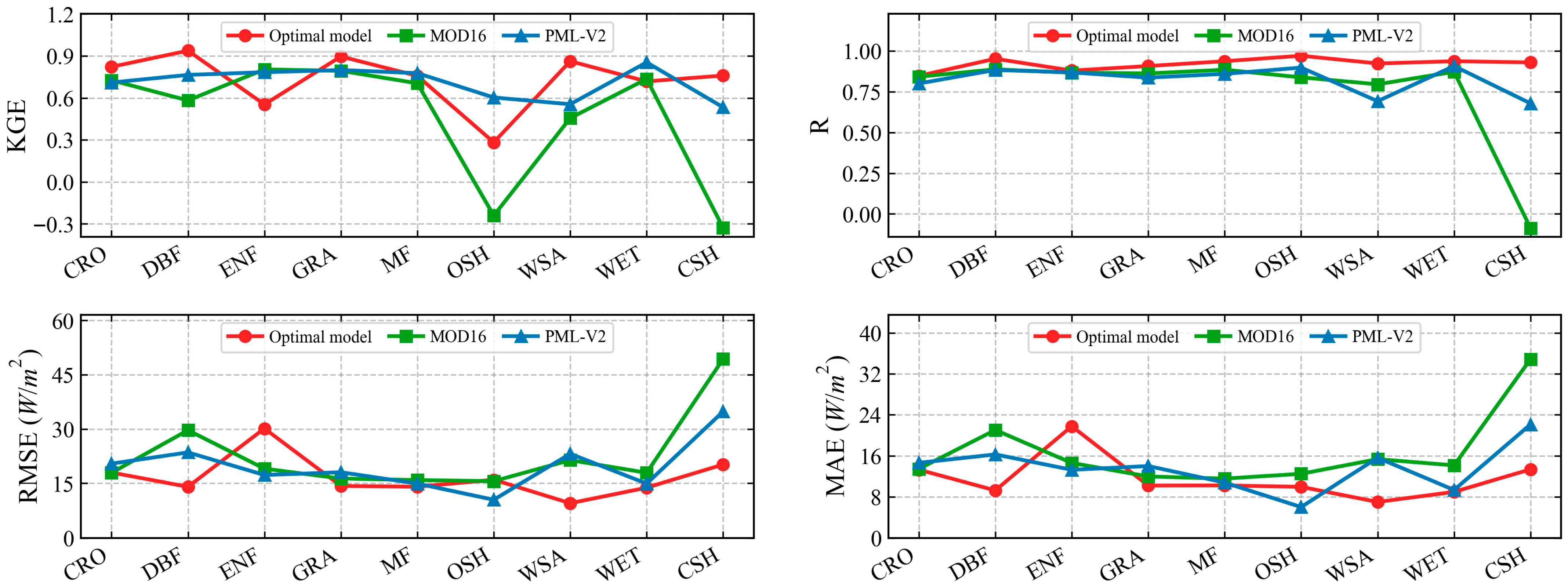
As shown in Figure 10, the optimal model exhibits higher simulation accuracy and better stability across most land cover types. PML-V2 shows the second-best performance, whereas MOD16 exhibits a clear decline in accuracy across several land cover types, particularly at the OSH and CSH sites.

5. Discussion

5.1. Effects of Canopy Conductance Structural Assumptions on Model Performance

To further identify the sources of model performance improvement, this study compared the optimal model (Equation (16)) with two representative model structures: one is the K95 model [29] (Equation (19)), which considers only canopy radiation attenuation; the other is the Jarvis model (Equation (20)), which applies the classic multiplicative limitation framework but scales conductance to the canopy by simply multiplying by LAI. In fact, all three models adopt the same PAR constraint function (Equation (21)):
G c = g s m k Q l n P A R + Q P A R e x p k Q L A I + Q
G c = L A I g s m f P A R f V P D f T f θ
f P A R = P A R P A R + Q
As shown in Figure 11, the optimal model yields an RMSE of 28.15 W/m2, an MAE of 18.84 W/m2, a KGE of 0.82, and an R of 0.82. Its scatter points cluster tightly around the 1:1 line, particularly within the main evapotranspiration range of 0–200 W/m2, indicating that the model reliably captures both the magnitude and variability of ET. In contrast, the K95 model shows a higher RMSE of 45.24 W/m2 and a reduced KGE of 0.61. The Jarvis model performs slightly better than K95, with a KGE of 0.71 and an RMSE of 31.96 W/m2, yet still falls short of the optimal model. This indicates that considering only radiation attenuation or applying environmental limitation factors through a multiplicative form alone is insufficient to fully capture the complexity of canopy evapotranspiration processes.
The accuracy differences among the models essentially arise from the incompleteness of their structural assumptions. The K95 model uses an exponential function to describe light attenuation within the canopy during upscaling, which physiologically captures the effect of leaf area on light absorption and maintains consistency with energy balance in terms of radiation partitioning [78]. However, the model lacks explicit representation of transpiration-suppressing factors and cannot dynamically regulate stomatal conductance under high temperature, high VPD, or soil moisture limitation, resulting in weakened stress responses in the ET process [79]. It often produces substantial overestimation or underestimation under high ET conditions, with increased scatter of simulated values, indicating that radiation transfer alone is insufficient to explain ET dynamics under extreme meteorological conditions. The Jarvis model uses an empirical multi-factor framework to represent the limiting effects of radiation, temperature, VPD, and soil moisture on stomatal conductance, providing strong generality [28]. However, when upscaled, the model does not explicitly consider canopy light attenuation or the vertical distribution of photosynthetically active radiation. As a result, it often overestimates light-use efficiency and peak ET in high-LAI vegetation types. This bias is particularly evident in forest and cropland canopies, where radiation stratification is strong [80].

5.2. Coupling Between Temperature and Vapor Pressure Deficit Functions

In this study, VPD is calculated from air temperature and dew-point temperature, so f V P D and f T are partly coupled. This coupling means that rising temperature directly affects the temperature limitation function f T , and also increases VPD, which indirectly strengthens the suppression by f V P D , causing their limiting effects to accumulate under high-temperature conditions. Yang et al. [81] observed in an Australian dry-forest site that when VPD exceeds 2 kPa, both photosynthesis and stomatal conductance decrease substantially. They also found that models ignoring the indirect effect of temperature on VPD systematically underestimate the strength of transpiration suppression. Experiments by Eze et al. [82] on tropical tree species showed that when VPD is held constant, the negative effect of warming on photosynthesis becomes much weaker. However, when VPD is allowed to rise with temperature, the decline in photosynthesis is mainly driven by VPD rather than temperature itself. Physiologically, increasing VPD raises evaporative demand, causing stomata to close rapidly to reduce the risk of water deficit. Warming further amplifies this process by increasing saturation vapor pressure [83]. Under extreme heat, the combined effect may even decouple stomatal conductance from photosynthesis. That is, stomatal closure becomes stronger than required for carbon assimilation, causing deviations in energy partitioning and evapotranspiration [84].
In the parameterization of stomatal conductance models, using independent f T and f V P D functions may lead to duplicated suppression under hot and dry conditions, thereby amplifying the uncertainty in model outputs. To improve physical consistency, future structural optimization may adopt a joint-constraint strategy, such as coupling functions based on air humidity or the saturation vapor pressure curve, to reduce the redundant responses of temperature and VPD and enhance model stability and explanatory power under extreme meteorological conditions.

6. Conclusions

This study developed an improved canopy conductance-based evapotranspiration (ET) estimation framework by coupling canopy radiation transfer with a multiplicative Jarvis model and explicitly accounting for PAR, vapor pressure deficit (VPD), air temperature, and soil moisture constraints. By constructing a representative structural space with 18 combinations of limitation functions and applying a two-stage optimization strategy across 79 sites (2015–2023) from 12 IGBP land cover types, we quantified structural sensitivity and identified land cover-specific optimal function combinations. Additionally, nine sites from nine different land cover types were selected for independent spatial validation. For the optimization sites, the model showed good agreement with tower latent heat flux (LE) at the daily scale, achieving KGE = 0.82, R = 0.82, and RMSE = 27.83 W/m2, indicating strong temporal stability. Over the spatially independent holdout sites, the model achieved KGE = 0.84, R = 0.84, and RMSE = 22.53 W/m2, confirming its transferability. At the 8-day scale, when evaluated over the holdout sites, the model further outperformed two widely used ET products (MOD16 and PML-V2), reaching KGE = 0.87 and RMSE = 18.74 W/m2, indicating improved temporal stability and reduced high-flux deviations. Comparisons against the traditional Jarvis and K95 model demonstrate that jointly representing canopy radiation transfer and multi-factor environmental limitations is essential for improving physiological realism and cross-land cover transferability in large-scale ET retrieval. Future work should further reduce potential redundancy between temperature and VPD constraints by exploring coupled stress formulations to enhance robustness under concurrent heat and atmospheric drought.
The improved canopy conductance model outperforms existing models in structural completeness, physiological consistency, and cross-land cover applicability. It provides a more robust theoretical basis and parameterization framework for regional and global evapotranspiration remote-sensing retrieval.

Author Contributions

Conceptualization, J.W., X.X. and S.Y.; methodology, J.W. and Z.Y.; software, J.W. and Z.Y.; validation, J.W., X.X. and S.Z.; formal analysis, J.W., X.X., T.L. and S.Z.; investigation, J.W. and S.Z.; resources, J.W.; data curation, J.W.; writing—original draft preparation, J.W.; writing—review and editing, J.W., X.X., S.Z., T.L. and S.Y.; visualization, J.W.; supervision, X.X. and S.Y.; project administration, X.X.; funding acquisition, X.X. All authors have read and agreed to the published version of the manuscript.

Funding

The study was supported by the National Key Research and Development Program of China (Grant No. 2023YFF1303602).

Data Availability Statement

The data used in this study are available in a publicly accessible repository.

Acknowledgments

We thank the providers of all observational datasets used in this article for making their data publicly accessible, and we also appreciate the reviewers and editors whose comments and suggestions have contributed to improving this paper.

Conflicts of Interest

Author Z.Y. was employed by China Information Security Research Institute Co., Ltd. The remaining authors declare that the research was conducted in the absence of any commercial or financial relationships that could be construed as a potential conflict of interest.

References

  1. Miralles, D.G.; Gash, J.H.; Holmes, T.R.H.; De Jeu, R.A.M.; Dolman, A.J. Global Canopy Interception from Satellite Observations. J. Geophys. Res. 2010, 115, 2009JD013530. [Google Scholar] [CrossRef]
  2. Stoy, P.C.; El-Madany, T.S.; Fisher, J.B.; Gentine, P.; Gerken, T.; Good, S.P.; Klosterhalfen, A.; Liu, S.; Miralles, D.G.; Perez-Priego, O.; et al. Reviews and Syntheses: Turning the Challenges of Partitioning Ecosystem Evaporation and Transpiration into Opportunities. Biogeosciences 2019, 16, 3747–3775. [Google Scholar] [CrossRef]
  3. Wang, Z.; Zhan, C.; Ning, L.; Guo, H. Evaluation of Global Terrestrial Evapotranspiration in CMIP6 Models. Theor. Appl. Climatol. 2021, 143, 521–531. [Google Scholar] [CrossRef]
  4. Zhang, Y.; Peña-Arancibia, J.L.; McVicar, T.R.; Chiew, F.H.S.; Vaze, J.; Liu, C.; Lu, X.; Zheng, H.; Wang, Y.; Liu, Y.Y.; et al. Multi-Decadal Trends in Global Terrestrial Evapotranspiration and Its Components. Sci. Rep. 2016, 6, 19124. [Google Scholar] [CrossRef]
  5. Allen, R.G.; Food and Agriculture Organization of the United Nations (Eds.) Crop Evapotranspiration: Guidelines for Computing Crop Water Requirements; FAO Irrigation and Drainage Paper; Food and Agriculture Organization of the United Nations: Rome, Italy, 1998. [Google Scholar]
  6. Miralles, D.G.; Holmes, T.R.H.; De Jeu, R.A.M.; Gash, J.H.; Meesters, A.G.C.A.; Dolman, A.J. Global Land-Surface Evaporation Estimated from Satellite-Based Observations. Hydrol. Earth Syst. Sci. 2011, 15, 453–469. [Google Scholar] [CrossRef]
  7. Li, Z.-L.; Tang, R.; Wan, Z.; Bi, Y.; Zhou, C.; Tang, B.; Yan, G.; Zhang, X. A Review of Current Methodologies for Regional Evapotranspiration Estimation from Remotely Sensed Data. Sensors 2009, 9, 3801–3853. [Google Scholar] [CrossRef]
  8. Hu, G.; Jia, L. Monitoring of Evapotranspiration in a Semi-Arid Inland River Basin by Combining Microwave and Optical Remote Sensing Observations. Remote Sens. 2015, 7, 3056–3087. [Google Scholar] [CrossRef]
  9. Zheng, C.; Jia, L.; Hu, G. Global Land Surface Evapotranspiration Monitoring by ETMonitor Model Driven by Multi-Source Satellite Earth Observations. J. Hydrol. 2022, 613, 128444. [Google Scholar] [CrossRef]
  10. Bastiaanssen, W.G.M.; Menenti, M.; Feddes, R.A.; Holtslag, A.A.M. A Remote Sensing Surface Energy Balance Algorithm for Land (SEBAL). 1. Formulation. J. Hydrol. 1998, 212–213, 198–212. [Google Scholar] [CrossRef]
  11. Su, Z. The Surface Energy Balance System (SEBS) for Estimation of Turbulent Heat Fluxes. Hydrol. Earth Syst. Sci. 2002, 6, 85–100. [Google Scholar] [CrossRef]
  12. Monteith, J.L. Evaporation and Environment. Symp. Soc. Exp. Biol. 1965, 19, 205–234. [Google Scholar]
  13. Michel, D.; Jiménez, C.; Miralles, D.G.; Jung, M.; Hirschi, M.; Ershadi, A.; Martens, B.; McCabe, M.F.; Fisher, J.B.; Mu, Q.; et al. The WACMOS-ET Project—Part 1: Tower-Scale Evaluation of Four Remote-Sensing-Based Evapotranspiration Algorithms. Hydrol. Earth Syst. Sci. 2016, 20, 803–822. [Google Scholar] [CrossRef]
  14. Long, D.; Longuevergne, L.; Scanlon, B.R. Global Analysis of Approaches for Deriving Total Water Storage Changes from GRACE Satellites. Water Resour. Res. 2015, 51, 2574–2594. [Google Scholar] [CrossRef]
  15. Zhang, K.; Kimball, J.S.; Running, S.W. A Review of Remote Sensing Based Actual Evapotranspiration Estimation. WIREs Water 2016, 3, 834–853. [Google Scholar] [CrossRef]
  16. Gerosa, G.; Mereu, S.; Finco, A.; Marzuoli, R. Stomatal Conductance Modeling to Estimate the Evapotranspiration of Natural and Agricultural Ecosystems. In Evapotranspiration—Remote Sensing and Modeling; Irmak, A., Ed.; InTech: London, UK, 2012. [Google Scholar]
  17. Pan, S.; Pan, N.; Tian, H.; Friedlingstein, P.; Sitch, S.; Shi, H.; Arora, V.K.; Haverd, V.; Jain, A.K.; Kato, E.; et al. Evaluation of Global Terrestrial Evapotranspiration Using State-of-the-Art Approaches in Remote Sensing, Machine Learning and Land Surface Modeling. Hydrol. Earth Syst. Sci. 2020, 24, 1485–1509. [Google Scholar] [CrossRef]
  18. Buckley, T.N. Modeling Stomatal Conductance. Plant Physiol. 2017, 174, 572–582. [Google Scholar] [CrossRef] [PubMed]
  19. Medlyn, B.E.; Duursma, R.A.; Eamus, D.; Ellsworth, D.S.; Prentice, I.C.; Barton, C.V.M.; Crous, K.Y.; De Angelis, P.; Freeman, M.; Wingate, L. Reconciling the Optimal and Empirical Approaches to Modelling Stomatal Conductance: RECONCILING OPTIMAL AND EMPIRICAL STOMATAL MODELS. Glob. Change Biol. 2011, 17, 2134–2144. [Google Scholar] [CrossRef]
  20. Jarvis, P.G. The Interpretation of the Variations in Leaf Water Potential and Stomatal Conductance Found in Canopies in the Field. Philos. Trans. R. Soc. London. B Biol. Sci. 1976, 273, 593–610. [Google Scholar] [CrossRef]
  21. Bai, Y.; Zhang, J.; Zhang, S.; Yao, F.; Magliulo, V. A Remote Sensing-Based Two-Leaf Canopy Conductance Model: Global Optimization and Applications in Modeling Gross Primary Productivity and Evapotranspiration of Crops. Remote Sens. Environ. 2018, 215, 411–437. [Google Scholar] [CrossRef]
  22. Lhomme, J.-P. Stomatal Control of Transpiration: Examination of the Jarvis-type Representation of Canopy Resistance in Relation to Humidity. Water Resour. Res. 2001, 37, 689–699. [Google Scholar] [CrossRef]
  23. Ball, J.T.; Woodrow, I.E.; Berry, J.A. A Model Predicting Stomatal Conductance and Its Contribution to the Control of Photosynthesis under Different Environmental Conditions. In Progress in Photosynthesis Research; Biggins, J., Ed.; Springer: Dordrecht, The Netherlands, 1987; pp. 221–224. [Google Scholar]
  24. Buckley, T.N.; Mott, K.A. Modelling Stomatal Conductance in Response to Environmental Factors. Plant Cell Environ. 2013, 36, 1691–1699. [Google Scholar] [CrossRef]
  25. Bu, J.; Gan, G.; Chen, J.; Su, Y.; García, M.; Gao, Y. Biophysical Constraints on Evapotranspiration Partitioning for a Conductance-Based Two Source Energy Balance Model. J. Hydrol. 2021, 603, 127179. [Google Scholar] [CrossRef]
  26. Bai, P.; Cai, C. Applicability Evaluation of Soil Moisture Constraint Algorithms in Remote Sensing Evapotranspiration Models. J. Hydrol. 2023, 623, 129870. [Google Scholar] [CrossRef]
  27. Guo, X.; Meng, D.; Chen, X.; Li, X. Validation and Comparison of Seven Land Surface Evapotranspiration Products in the Haihe River Basin, China. Remote Sens. 2022, 14, 4308. [Google Scholar] [CrossRef]
  28. Shao, W.; Li, M.; Su, Y.; Gao, H.; Vlček, L. A Modified Jarvis Model to Improve the Expressing of Stomatal Response in a Beech Forest. Hydrol. Process. 2023, 37, e14955. [Google Scholar] [CrossRef]
  29. Kelliher, F.M.; Leuning, R.; Raupach, M.R.; Schulze, E.-D. Maximum Conductances for Evaporation from Global Vegetation Types. Agric. For. Meteorol. 1995, 73, 1–16. [Google Scholar] [CrossRef]
  30. Sellers, P.J.; Dickinson, R.E.; Randall, D.A.; Betts, A.K.; Hall, F.G.; Berry, J.A.; Collatz, G.J.; Denning, A.S.; Mooney, H.A.; Nobre, C.A.; et al. Modeling the Exchanges of Energy, Water, and Carbon Between Continents and the Atmosphere. Science 1997, 275, 502–509. [Google Scholar] [CrossRef]
  31. Mu, Q.; Heinsch, F.A.; Zhao, M.; Running, S.W. Development of a Global Evapotranspiration Algorithm Based on MODIS and Global Meteorology Data. Remote Sens. Environ. 2007, 111, 519–536. [Google Scholar] [CrossRef]
  32. Mu, Q.; Zhao, M.; Running, S.W. Improvements to a MODIS Global Terrestrial Evapotranspiration Algorithm. Remote Sens. Environ. 2011, 115, 1781–1800. [Google Scholar] [CrossRef]
  33. Bonan, G.B.; Williams, M.; Fisher, R.A.; Oleson, K.W. Modeling Stomatal Conductance in the Earth System: Linking Leaf Water-Use Efficiency and Water Transport along the Soil–Plant–Atmosphere Continuum. Geosci. Model Dev. 2014, 7, 2193–2222. [Google Scholar] [CrossRef]
  34. Wang, K.; Dickinson, R.E. A Review of Global Terrestrial Evapotranspiration: Observation, Modeling, Climatology, and Climatic Variability. Rev. Geophys. 2012, 50, 2011RG000373. [Google Scholar] [CrossRef]
  35. De Kauwe, M.G.; Medlyn, B.E.; Zaehle, S.; Walker, A.P.; Dietze, M.C.; Wang, Y.; Luo, Y.; Jain, A.K.; El-Masri, B.; Hickler, T.; et al. Where Does the Carbon Go? A Model–Data Intercomparison of Vegetation Carbon Allocation and Turnover Processes at Two Temperate Forest Free-air CO2 Enrichment Sites. N. Phytol. 2014, 203, 883–899. [Google Scholar] [CrossRef]
  36. Bonan, G.B.; Doney, S.C. Climate, Ecosystems, and Planetary Futures: The Challenge to Predict Life in Earth System Models. Science 2018, 359, eaam8328. [Google Scholar] [CrossRef]
  37. Martens, B.; Miralles, D.G.; Lievens, H.; Van Der Schalie, R.; De Jeu, R.A.M.; Férnandez-Prieto, D.; Beck, H.E.; Dorigo, W.A.; Verhoest, N.E.C. GLEAM v3: Satellite-Based Land Evaporation and Root-Zone Soil Moisture. Geosci. Model Dev. 2017, 10, 1903–1925. [Google Scholar] [CrossRef]
  38. Knauer, J.; Zaehle, S.; Medlyn, B.E.; Reichstein, M.; Williams, C.A.; Migliavacca, M.; De Kauwe, M.G.; Werner, C.; Keitel, C.; Kolari, P.; et al. Towards Physiologically Meaningful Water-use Efficiency Estimates from Eddy Covariance Data. Glob. Change Biol. 2018, 24, 694–710. [Google Scholar] [CrossRef] [PubMed]
  39. Restrepo-Coupe, N.; Da Rocha, H.R.; Hutyra, L.R.; Da Araujo, A.C.; Borma, L.S.; Christoffersen, B.; Cabral, O.M.R.; De Camargo, P.B.; Cardoso, F.L.; Da Costa, A.C.L.; et al. What Drives the Seasonality of Photosynthesis across the Amazon Basin? A Cross-Site Analysis of Eddy Flux Tower Measurements from the Brasil Flux Network. Agric. For. Meteorol. 2013, 182–183, 128–144. [Google Scholar] [CrossRef]
  40. Pastorello, G.; Trotta, C.; Canfora, E.; Chu, H.; Christianson, D.; Cheah, Y.-W.; Poindexter, C.; Chen, J.; Elbashandy, A.; Humphrey, M.; et al. The FLUXNET2015 Dataset and the ONEFlux Processing Pipeline for Eddy Covariance Data. Sci. Data 2020, 7, 225. [Google Scholar] [CrossRef]
  41. Yan, K.; Wang, J.; Weiss, M.; Myneni, R.B. A High-Quality Reprocessed MODIS Leaf Area Index Dataset (HiQ-LAI). 2023. Available online: https://zenodo.org/records/8296768 (accessed on 21 May 2025).
  42. Chen, J.; Jönsson, P.; Tamura, M.; Gu, Z.; Matsushita, B.; Eklundh, L. A Simple Method for Reconstructing a High-Quality NDVI Time-Series Data Set Based on the Savitzky–Golay Filter. Remote Sens. Environ. 2004, 91, 332–344. [Google Scholar] [CrossRef]
  43. Reichle, R.H.; De Lannoy, G.J.M.; Liu, Q.; Ardizzone, J.V.; Colliander, A.; Conaty, A.; Crow, W.; Jackson, T.J.; Jones, L.A.; Kimball, J.S.; et al. Assessment of the SMAP Level-4 Surface and Root-Zone Soil Moisture Product Using In Situ Measurements. J. Hydrometeorol. 2017, 18, 2621–2645. [Google Scholar] [CrossRef]
  44. Zhang, Y.; Schaap, M.G.; Wei, Z. Development of Hierarchical Ensemble Model and Estimates of Soil Water Retention with Global Coverage. Geophys. Res. Lett. 2020, 47, e2020GL088819. [Google Scholar] [CrossRef]
  45. Chen, X.; Su, Z.; Ma, Y.; Yang, K.; Wang, B. Estimation of Surface Energy Fluxes under Complex Terrain of Mt. Qomolangma over the Tibetan Plateau. Hydrol. Earth Syst. Sci. 2013, 17, 1607–1618. [Google Scholar] [CrossRef]
  46. Fisher, J.B.; Tu, K.P.; Baldocchi, D.D. Global Estimates of the Land–Atmosphere Water Flux Based on Monthly AVHRR and ISLSCP-II Data, Validated at 16 FLUXNET Sites. Remote Sens. Environ. 2008, 112, 901–919. [Google Scholar] [CrossRef]
  47. Yan, H.; Wang, S.Q.; Billesbach, D.; Oechel, W.; Zhang, J.H.; Meyers, T.; Martin, T.A.; Matamala, R.; Baldocchi, D.; Bohrer, G.; et al. Global Estimation of Evapotranspiration Using a Leaf Area Index-Based Surface Energy and Water Balance Model. Remote Sens. Environ. 2012, 124, 581–595. [Google Scholar] [CrossRef]
  48. Purdy, A.J.; Fisher, J.B.; Goulden, M.L.; Colliander, A.; Halverson, G.; Tu, K.; Famiglietti, J.S. SMAP Soil Moisture Improves Global Evapotranspiration. Remote Sens. Environ. 2018, 219, 1–14. [Google Scholar] [CrossRef]
  49. Massman, W.J. A Model Study of kBH−1 for Vegetated Surfaces Using ‘Localized near-Field’ Lagrangian Theory. J. Hydrol. 1999, 223, 27–43. [Google Scholar] [CrossRef]
  50. Lindroth, A.; Mölder, M.; Lagergren, F. Heat Storage in Forest Biomass Improves Energy Balance Closure. Biogeosciences 2010, 7, 301–313. [Google Scholar] [CrossRef]
  51. Moderow, U.; Aubinet, M.; Feigenwinter, C.; Kolle, O.; Lindroth, A.; Mölder, M.; Montagnani, L.; Rebmann, C.; Bernhofer, C. Available Energy and Energy Balance Closure at Four Coniferous Forest Sites across Europe. Theor. Appl. Climatol. 2009, 98, 397–412. [Google Scholar] [CrossRef]
  52. Zhang, Y.; Leuning, R.; Hutley, L.B.; Beringer, J.; McHugh, I.; Walker, J.P. Using Long-term Water Balances to Parameterize Surface Conductances and Calculate Evaporation at 0.05° Spatial Resolution. Water Resour. Res. 2010, 46, 2009WR008716. [Google Scholar] [CrossRef]
  53. García-Gutiérrez, V.; Stöckle, C.; Gil, P.M.; Meza, F.J. Evaluation of Penman-Monteith Model Based on Sentinel-2 Data for the Estimation of Actual Evapotranspiration in Vineyards. Remote Sens. 2021, 13, 478. [Google Scholar] [CrossRef]
  54. Chen, X.; Su, Z.; Ma, Y.; Trigo, I.; Gentine, P. Remote Sensing of Global Daily Evapotranspiration Based on a Surface Energy Balance Method and Reanalysis Data. JGR Atmos. 2021, 126, e2020JD032873. [Google Scholar] [CrossRef]
  55. Wehr, R.; Saleska, S.R. Calculating Canopy Stomatal Conductance from Eddy Covariance Measurements, in Light of the Energy Budget Closure Problem. Biogeosciences 2021, 18, 13–24. [Google Scholar] [CrossRef]
  56. Flo, V.; Martínez-Vilalta, J.; Granda, V.; Mencuccini, M.; Poyatos, R. Vapour Pressure Deficit Is the Main Driver of Tree Canopy Conductance across Biomes. Agric. For. Meteorol. 2022, 322, 109029. [Google Scholar] [CrossRef]
  57. Wu, R.-Q.; Jia, J.-B.; Yan, W.-D.; Hu, L.; Wang, Y.-F.; Chen, Y. Characteristics of Canopy Conductance and Environmental Driving Mechanism in Three Monsoon Climate Regions of China. Front. Environ. Sci. 2022, 10, 935926. [Google Scholar] [CrossRef]
  58. Leuning, R.; Zhang, Y.Q.; Rajaud, A.; Cleugh, H.; Tu, K. A Simple Surface Conductance Model to Estimate Regional Evaporation Using MODIS Leaf Area Index and the Penman-Monteith Equation. Water Resour. Res. 2008, 44, 2007WR006562. [Google Scholar] [CrossRef]
  59. Grossiord, C.; Buckley, T.N.; Cernusak, L.A.; Novick, K.A.; Poulter, B.; Siegwolf, R.T.W.; Sperry, J.S.; McDowell, N.G. Plant Responses to Rising Vapor Pressure Deficit. New Phytol. 2020, 226, 1550–1566. [Google Scholar] [CrossRef]
  60. Slot, M.; Rifai, S.W.; Eze, C.E.; Winter, K. The Stomatal Response to Vapor Pressure Deficit Drives the Apparent Temperature Response of Photosynthesis in Tropical Forests. New Phytol. 2024, 244, 1238–1249. [Google Scholar] [CrossRef] [PubMed]
  61. Wedegaertner, K.; Shekoofa, A.; Purdom, S.; Walters, K.; Duncan, L.; Raper, T.B. Cotton Stomatal Closure under Varying Temperature and Vapor Pressure Deficit, Correlation with the Hydraulic Conductance Trait. J. Cotton Res. 2022, 5, 20. [Google Scholar] [CrossRef]
  62. Anav, A.; Proietti, C.; Menut, L.; Carnicelli, S.; De Marco, A.; Paoletti, E. Sensitivity of Stomatal Conductance to Soil Moisture: Implications for Tropospheric Ozone. Atmos. Chem. Phys. 2018, 18, 5747–5763. [Google Scholar] [CrossRef]
  63. Wood, J.D.; Gu, L.; Hanson, P.J.; Frankenberg, C.; Sack, L. The Ecosystem Wilting Point Defines Drought Response and Recovery of a quercus-carya Forest. Glob. Change Biol. 2023, 29, 2015–2029. [Google Scholar] [CrossRef]
  64. Ortega-Farias, S.; Poblete-Echeverría, C.; Brisson, N. Parameterization of a Two-Layer Model for Estimating Vineyard Evapotranspiration Using Meteorological Measurements. Agric. For. Meteorol. 2010, 150, 276–286. [Google Scholar] [CrossRef]
  65. Samanta, S.; Mackay, D.S.; Clayton, M.K.; Kruger, E.L.; Ewers, B.E. Bayesian Analysis for Uncertainty Estimation of a Canopy Transpiration Model. Water Resour. Res. 2007, 43, 2006WR005028. [Google Scholar] [CrossRef]
  66. Li, S.; Kang, S.; Zhang, L.; Li, F.; Hao, X.; Ortega-Farias, S.; Guo, W.; Ji, S.; Wang, J.; Jiang, X. Quantifying the Combined Effects of Climatic, Crop and Soil Factors on Surface Resistance in a Maize Field. J. Hydrol. 2013, 489, 124–134. [Google Scholar] [CrossRef]
  67. Ding, R.; Kang, S.; Du, T.; Hao, X.; Tong, L. Modeling Crop Water Use in an Irrigated Maize Cropland Using a Biophysical Process-Based Model. J. Hydrol. 2015, 529, 276–286. [Google Scholar] [CrossRef]
  68. Gupta, H.V.; Kling, H.; Yilmaz, K.K.; Martinez, G.F. Decomposition of the Mean Squared Error and NSE Performance Criteria: Implications for Improving Hydrological Modelling. J. Hydrol. 2009, 377, 80–91. [Google Scholar] [CrossRef]
  69. Körner, C. Leaf Diffusive Conductances in the Major Vegetation Types of the Globe. In Ecophysiology of Photosynthesis; Schulze, E.-D., Caldwell, M.M., Eds.; Springer: Berlin/Heidelberg, Germany, 1995; pp. 463–490. [Google Scholar]
  70. Wilson, K.; Goldstein, A.; Falge, E.; Aubinet, M.; Baldocchi, D.; Berbigier, P.; Bernhofer, C.; Ceulemans, R.; Dolman, H.; Field, C.; et al. Energy Balance Closure at FLUXNET Sites. Agric. For. Meteorol. 2002, 113, 223–243. [Google Scholar] [CrossRef]
  71. Mauder, M.; Foken, T.; Cuxart, J. Surface-Energy-Balance Closure over Land: A Review. Bound. Layer Meteorol. 2020, 177, 395–426. [Google Scholar] [CrossRef]
  72. Zhao, W.; Li, A. A Review on Land Surface Processes Modelling over Complex Terrain. Adv. Meteorol. 2015, 2015, 1–17. [Google Scholar] [CrossRef]
  73. Overgaard, J.; Rosbjerg, D.; Butts, M.B. Land-Surface Modelling in Hydrological Perspective—A Review. Biogeosciences 2006, 3, 229–241. [Google Scholar] [CrossRef]
  74. Pal, S.; Sharma, P. A Review of Machine Learning Applications in Land Surface Modeling. Earth 2021, 2, 174–190. [Google Scholar] [CrossRef]
  75. Ting, S.; Lymburn, T.; Stemler, T.; Sun, Y.; Small, M. Model Calibration and Validation from a Statistical Inference Perspective. arXiv 2023, arXiv:2309.08562. [Google Scholar] [CrossRef]
  76. Mayr, S.; Kuenzer, C.; Gessner, U.; Klein, I.; Rutzinger, M. Validation of Earth Observation Time-Series: A Review for Large-Area and Temporally Dense Land Surface Products. Remote Sens. 2019, 11, 2616. [Google Scholar] [CrossRef]
  77. Zhang, Y.; Kong, D.; Gan, R.; Chiew, F.H.S.; McVicar, T.R.; Zhang, Q.; Yang, Y. Coupled Estimation of 500 m and 8-Day Resolution Global Evapotranspiration and Gross Primary Production in 2002–2017. Remote Sens. Environ. 2019, 222, 165–182. [Google Scholar] [CrossRef]
  78. Leuning, R. A Critical Appraisal of a Combined Stomatal-photosynthesis Model for C3 Plants. Plant Cell Environ. 1995, 18, 339–355. [Google Scholar] [CrossRef]
  79. Wang, Y.-P.; Leuning, R. A Two-Leaf Model for Canopy Conductance, Photosynthesis and Partitioning of Available Energy I:: Model Description and Comparison with a Multi-Layered Model. Agric. For. Meteorol. 1998, 91, 89–111. [Google Scholar] [CrossRef]
  80. Alam, M.S.; Lamb, D.W.; Warwick, N.W.M. A Canopy Transpiration Model Based on Scaling Up Stomatal Conductance and Radiation Interception as Affected by Leaf Area Index. Water 2021, 13, 252. [Google Scholar] [CrossRef]
  81. Yang, J.; Duursma, R.A.; De Kauwe, M.G.; Kumarathunge, D.; Jiang, M.; Mahmud, K.; Gimeno, T.E.; Crous, K.Y.; Ellsworth, D.S.; Peters, J.; et al. Incorporating Non-Stomatal Limitation Improves the Performance of Leaf and Canopy Models at High Vapour Pressure Deficit. Tree Physiol. 2019, 39, 1961–1974. [Google Scholar] [CrossRef]
  82. Eze, C.E.; Winter, K.; Slot, M. Vapor-Pressure-Deficit-Controlled Temperature Response of Photosynthesis in Tropical Trees. Photosynthetica 2024, 62, 318–325. [Google Scholar] [CrossRef]
  83. López, J.; Way, D.A.; Sadok, W. Systemic Effects of Rising Atmospheric Vapor Pressure Deficit on Plant Physiology and Productivity. Glob. Change Biol. 2021, 27, 1704–1720. [Google Scholar] [CrossRef]
  84. Marchin, R.M.; Medlyn, B.E.; Tjoelker, M.G.; Ellsworth, D.S. Decoupling Between Stomatal Conductance and Photosynthesis Occurs under Extreme Heat in Broadleaf Tree Species Regardless of Water Access. Glob. Change Biol. 2023, 29, 6319–6335. [Google Scholar] [CrossRef]
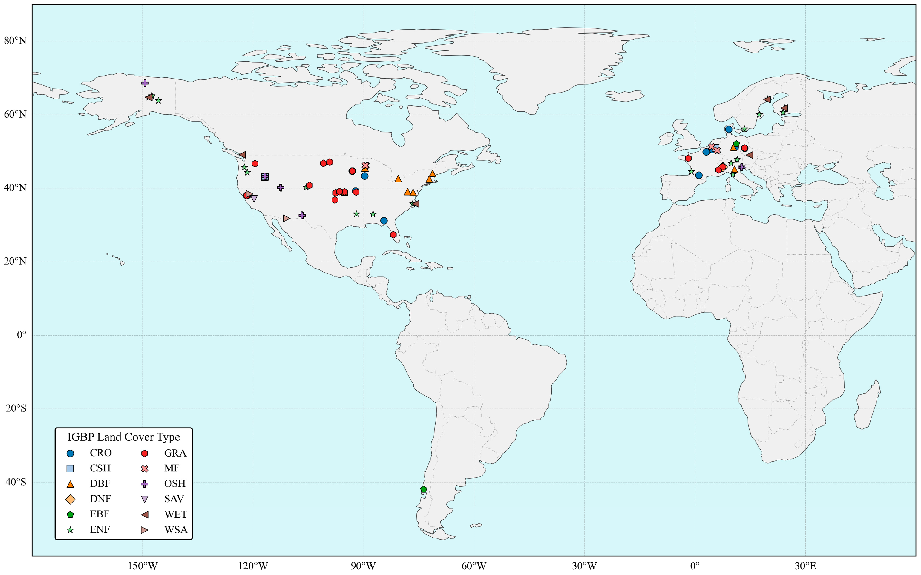
Figure 1. Distribution of flux sites. CRO: croplands; GRA: grasslands; CSH: closed shrublands; MF: mixed forests; DBF: deciduous broadleaf forests; OSH: open shrublands; DNF: deciduous needleleaf forests; SAV: savannas; EBF: evergreen broadleaf forests; WET: wetlands; ENF: evergreen needleleaf forests; and WSA: woody savannas.
Remotesensing 18 00513 g001
Figure 2. Overall performance of different function combinations across different land cover types.
Remotesensing 18 00513 g002
Figure 3. Detailed accuracy metrics of different limitation-function combinations optimized for different land cover types. The combination code “Mxyz” represents the combination of limiting functions, where x corresponds to the temperature function (T1 or T2), y corresponds to the VPD function (V1, V2, or V3), and z corresponds to the soil moisture function (W1, W2, or W3). For example, M231 denotes the combination T2 + V3 + W1.
Remotesensing 18 00513 g003
Figure 4. The comparison of the optimal model before and after the two optimization stages.
Remotesensing 18 00513 g004
Figure 5. Temporal validation results within optimization sites for LE estimation using the optimal conductance model. N is the number of samples in the comparison. The color bar represents the density of scatter points.
Remotesensing 18 00513 g005
Figure 6. Time series of typical optimization sites across different land cover types, where black dots represent observations, red solid lines indicate simulations, and the blue dashed line separates calibration data (left) from validation data (right).
Remotesensing 18 00513 g006
Figure 7. Scatter plot of observed versus simulated LE over holdout sites. The color bar represents the density of scatter points.
Remotesensing 18 00513 g007
Figure 8. Time series of typical holdout sites across different land cover types, where black dots represent observations and the red solid lines indicate simulations.
Remotesensing 18 00513 g008
Figure 9. Comparison between the proposed model and the MOD16 and PML-V2 products at the 8-day scale. The color bar represents the density of scatter points.
Remotesensing 18 00513 g009
Figure 10. Comparison of the optimal model with the MOD16 and PML-V2 products at 9 holdout sites of different land cover types.
Remotesensing 18 00513 g010
Figure 11. Comparison between the optimal model and the K95 and Jarvis models.
Remotesensing 18 00513 g011
Table 1. Specific information regarding the selection of different constraint functions.
Constraint FunctionLetterParameterDescriptionBoundSource
f T = T a c T c b / b a b a c b c b / b a T1aAir temperature when f(T) equals 0−10–0Zheng et al. [9]
bAir temperature when f(T) equals 120–30
cAir temperature when f(T) equals 030–40
f T = 1 d T e 2 T2dEmpirical coefficient0–0.005Ortega-Farias et al. [64]
eEmpirical coefficient0–50
f V P D = 1 V P D + D 50 V1 D 50 VPD when g s is half its maximum value0.3–5Samanta et al. [65]
f V P D = e m V P D V2mEmpirical coefficient0–1Li et al. [66]
f V P D = 1 n V P D V3nEmpirical coefficient0–0.5Samanta et al. [65]
f θ = θ 1 + x θ + x W1xEmpirical coefficient0.01–2Preliminary calculation
f θ = θ θ w p θ + θ f c W2 θ w p Wilting point-ESWRGC dataset
θ f c Field capacity-
f θ = 1 e y θ θ w p θ + θ f c W3yEmpirical coefficient0.1–5Ding et al. [67]
Table 2. Optimal models and their accuracy metrics for different land cover types.
IGBP ClassOptimal ModelKGERRMSEMAE
ENFM2210.780.7830.119.6
EBFM2310.790.7928.520.9
DNFM2210.870.9015.611.6
DBFM2310.860.8627.417.9
MFM2310.910.9118.813.1
CROM2310.820.8331.121.6
GRAM2310.820.8230.520.8
OSHM2210.680.7822.515.5
CSHM2210.860.8622.816.4
SAVM2210.770.7814.911.0
WSAM1310.780.7818.113.1
WETM2310.850.8626.818.3
Disclaimer/Publisher’s Note: The statements, opinions and data contained in all publications are solely those of the individual author(s) and contributor(s) and not of MDPI and/or the editor(s). MDPI and/or the editor(s) disclaim responsibility for any injury to people or property resulting from any ideas, methods, instructions or products referred to in the content.